High-dimensional parameter optimization of a biogeochemical model: a multi-variable BGC-Argo data assimilation approach

The predictive accuracy of marine biogeochemical models is limited by uncertainty in their parameter values. We present a parameter optimization framework using iterative Importance Sampling (iIS) to constrain the PISCES biogeochemical model within a one-dimensional representation of the ocean by leveraging the comprehensive, multi-variable dataset provided by Biogeochemical-Argo (BGC-Argo) floats. Using seasonal observations from a single BGC-Argo float in the North Atlantic during the year 2015, we assimilate twenty observational quantities derived from eight biogeochemical tracers to directly optimise all 95 poorly known model parameters. A prerequisite global sensitivity analysis (GSA) identifies parameters controlling zooplankton dynamics as the dominant source of model sensitivity at this site. We compare three strategies: (1) optimising a subset of parameters selected for their strong direct influence (Main effects); (2) optimising a larger subset that also includes parameters influential through non-linear interactions (Total effects); and (3) simultaneously optimising all 95 parameters. All three approaches achieve a statistically indistinguishable goodness of fit to the assimilated observations, reducing the median normalised RMSE across metrics by 54 %–56 % relative to the reference simulation with default PISCES parameters. The comprehensive, multi-variable observational constraint yields posterior parameter distributions with negligible inter-parameter correlation, shifting the long-standing challenge of correlated equifinality to uncorrelated equifinality: multiple optimal parameter sets exist, but the individual parameters are uncorrelated rather than compensating for one another. Parameter uncertainty is reduced by 16 %–41 % relative to the broad uniform prior distributions. While all strategies produce a similar goodness of fit for the assimilated variables, they differ in computational cost and in their estimation of uncertainty for unassimilated variables. The All-parameters strategy provides a fuller accounting of parametric uncertainty for unassimilated variables, because it allows all parameters to vary rather than artificially fixing poorly known parameters at their default values. The method is computationally tractable thanks to the use of a one-dimensional model configuration, requiring approximately 24 CPU-hours for the optimization step, whereas the prerequisite GSA was ∼ 40 times more computationally expensive. When implemented in the three-dimensional IBI (Iberian–Biscay–Irish) regional model at $\mathrm{1}/\mathrm{36}$° resolution over a three-year period (2017–2019), the optimized parameter set from the All-parameters strategy improves the overall normalised RMSE against approximately 1430 independent BGC-Argo vertical profiles of nutrients and carbonates, although nitrate and silicate show degraded skill in the Mediterranean. Surface chlorophyll a is also better reproduced across the domain, when evaluated against a multi-observation reprocessed product. The generality of the approach should be tested by applying it to additional BGC-Argo floats in other oceanic regions.

1 Introduction

Since the beginning of industrialization, the world's oceans have absorbed approximately 26 % of anthropogenic carbon dioxide (CO₂) emissions (Friedlingstein et al., 2023), leading to profound changes in marine ecosystems. This increased CO₂ uptake is driving ocean acidification, which alters ocean chemistry (Doney et al., 2009), harms calcifying organisms (Orr et al., 2005), and disrupts broader biogeochemical processes (Hoegh-Guldberg et al., 2017). Concurrently, global deoxygenation, exacerbated by rising temperatures and ocean stratification (Keeling et al., 2010), is expanding oxygen minimum zones (Stramma et al., 2008), posing significant threats to marine life (Breitburg et al., 2018; Limburg et al., 2020). These challenges are further compounded by more direct anthropogenic impacts, such as plastic pollution (Wilcox et al., 2015) and overfishing (Pauly et al., 2002) which disrupt food webs (Dulvy et al., 2021) and degrade marine habitats (MacLeod et al., 2021).

Numerical biogeochemical (BGC) models are essential tools for understanding, monitoring, predicting, and mitigating these human-induced changes (Fennel et al., 2022). These models simulate key three-dimensional ocean processes, such as nutrient and plankton dynamics and carbon cycling, for past, present, and future ocean conditions. By capturing the complex interactions among physical, chemical, and biological components of the marine environment, BGC models produce critical outputs that supports scientific research, inform environmental management strategies, and guide policy development to conserve marine ecosystems (Fennel et al., 2019).

The accuracy of Ocean BGC models is limited by the uncertainty in their parameter values. This affects their predictive skill, particularly when it comes to monitoring the ocean carbon sink (Mayot et al., 2024) and for climate projections of the biological carbon pump framework. This parameter uncertainty stems from multiple sources. Many parameters are extrapolated from laboratory experiments using a limited selection of representative species or even specific laboratory strains; while this approach provides valuable insights, it falls short in simulations of diverse oceanic bioregions that host a vast diversity of organisms (Ward et al., 2010; Schartau et al., 2017). Furthermore, some parameters cannot be experimentally determined and are thus assigned wide plausible ranges. The resulting parametric uncertainty can be substantial (Schartau et al., 2017), which propagates to uncertainty in model predictions. Therefore, refining these model parameters is essential to improve the accuracy and reliability of BGC models.

It should be noted that structural uncertainty – arising from simplifications in the model's process formulations – is an additional source of error that parameter optimization alone cannot address. The present study focuses on parametric uncertainty, which can be systematically reduced through data assimilation.

To address parameter uncertainty, the ocean biogeochemical modeling community has increasingly relied on data assimilation techniques that leverage observational data to constrain model parameters (Dowd et al., 2014; Schartau et al., 2017; Fennel et al., 2022). This process typically begins with a sensitivity analysis to identify the most influential parameters (Chu et al., 2007). Parameters with minimal influence on model outcomes are fixed at reference values, while only the influential control parameters are subsequently adjusted, usually around their nominal values. This common strategy, often based on local sensitivity analysis, is computationally efficient but fails to capture behavior across the entire parameter space or account for parameter interactions and other non-linear effects.

Global sensitivity analysis (GSA) is a method that captures complex nonlinear interactions among parameters (Homma and Saltelli, 1996; Sobol', 2001). Historically, the extensive computational demands of GSA restricted its practical use, but recent increases in computing power have broadened its accessibility. Sobol' indices, a key GSA technique, quantify the influence of individual parameters and their interactions by apportioning the model output's variance among them. Prieur et al. (2019) applied this method to the MODECOGeL biogeochemical model which has 74 parameters (Lacroix and Grégoire, 2002). They found that nearly every parameter significantly affected model behavior, largely through intricate non-linear interactions rather than solely through direct effects on model outputs. By contrast, a gradient-based analysis of the same model highlighted only two influential parameters, overlooking the dependencies revealed by the GSA. This finding implies that parameter optimization efforts should include a large number of parameters to effectively reduce model-observation misfit. Furthermore, it underscores the limitations of traditional gradient-based optimization methods, which may fail to account for the broad impact of nonlinear parameter interactions.

Fulfilling the need to optimize many parameters, however, requires comprehensive, multi-variable observations. Traditional data sources, such as time-series stations and ocean-color satellite products, often lack the information content needed to constrain the large parameter sets of modern BGC models (Matear, 1995; Hurtt and Armstrong, 1996; Fennel et al., 2001; Friedrichs et al., 2007; Ward et al., 2010; Mamnun et al., 2022). Their vertical and temporal resolutions are too coarse, and the suite of measured variables too narrow, to fully inform the models (Fennel et al., 2022). Consequently, parameter-estimation studies based on such data frequently yield strong parameter correlations (Matear, 1995; Fennel et al., 2001; Mamnun et al., 2022), large posterior uncertainties (Ward et al., 2010), and optimized parameter sets that fail to reproduce independent observations (Friedrichs et al., 2007). Fundamentally, any one of these outcomes indicates that the assimilated data lack sufficient independent information to constrain each parameter independently.

BGC-Argo floats have revolutionized the acquisition of biogeochemical data by providing unprecedented data density at high vertical and temporal resolutions, while complementing the broad spatial coverage of traditional data sources (Claustre et al., 2020). These floats directly measure variables that correspond to key model state variables, including nitrate, chlorophyll a, oxygen (Mignot et al., 2023), and particulate organic carbon (POC) – which represents the total biomass of phytoplankton, micro-zooplankton, and small detritus (Galí et al., 2022). Furthermore, the CANYON-B neural network (Bittig et al., 2018) can infer silicate, phosphate, dissolved inorganic carbon, and alkalinity from direct BGC-Argo measurements (oxygen, temperature, salinity), significantly expanding the suite of available float-derived biogeochemical information. These high-resolution profiles also illuminate seasonally variable phenomena such as the precise onset of the North Atlantic bloom (Mignot et al., 2018). Because the profiles extend well below the euphotic zone, BGC-Argo data also resolve key vertical structures like the nitracline depth, deep-chlorophyll maxima (DCM), and oxygen-minimum zones (Mignot et al., 2014, 2023; Cornec et al., 2021; Bock et al., 2022; Liu et al., 2024). Each of these emergent properties provides a distinct constraint on different sets of model parameters. Dedicated scientific studies have quantified uncertainty estimates for each variable (Johnson et al., 2017; Mignot et al., 2019), supplying the error statistics required for robust data assimilation. Overall, BGC-Argo floats supply a more comprehensive information set than other types of in situ datasets, combining multi-variable breadth, high temporal resolution (∼ 5 d profiling versus monthly bottle sampling), and high vertical resolution (1 m grid versus discrete depths). This greater information content should allow many more model parameters to be constrained. However, to date, parameter optimization studies have used BGC-Argo data primarily for chlorophyll a and/or POC (Wang et al., 2020; Galí et al., 2022; Shu et al., 2022) no study has yet exploited the full suite of variables

In this study, we develop and apply a framework to optimise the 95 parameters of the Pelagic Interaction Scheme for Carbon and Ecosystem Studies (PISCES) biogeochemical model (Aumont et al., 2015) by assimilating the full suite of observations from a single BGC-Argo float over one seasonal cycle (January 2015–January 2016) in the North Atlantic. Our focus on this region is motivated by its role in the global carbon cycle (Takahashi et al., 2009; DeVries et al., 2014), and by the fact that PISCES, despite its extensive use in operational (e.g., Copernicus Marine Service) and climate (e.g., CMIP6) applications, exhibits systematic biases there. These biases are particularly evident in the seasonal cycles of key biogeochemical processes such as net primary production and pCO2 (Rodgers et al., 2023; Hieronymus et al., 2024).

The optimization is performed using iterative Importance Sampling (iIS), a Bayesian method that iteratively refines an ensemble of model simulations by reweighting parameter sets according to their agreement with the observations. At each iteration, the ensemble is concentrated towards the regions of parameter space that best reproduce the data, yielding full posterior distributions of parameters, including uncertainties and correlations.

A central objective of this work is to identify the most effective and efficient parameter-selection strategy for such a high-dimensional problem. We therefore evaluate and compare three distinct approaches:

• Main Effects: Optimizing a parameter subset based on first-order Sobol' indices from a GSA. This strategy targets parameters that have a significant direct effect on model output, independent of other parameters.

• Total Effects: Optimizing a larger subset based on total-order Sobol' indices. This strategy also includes parameters that are influential primarily through non-linear interactions with other parameters.

• All Parameters: Optimizing all 95 model parameters simultaneously, providing a computationally simple alternative that bypasses the prerequisite GSA.

Finally, a recurring question in biogeochemical optimization is whether parameters estimated in 1D configurations improve three-dimensional models, or if they merely compensate for missing physical processes (Löptien and Dietze, 2019; Pasquier et al., 2023). To address this, we assess the transferability of the optimization results by implementing the fully optimized parameter set into a high-resolution ($\mathrm{1}/\mathrm{36}$°) 3D regional model of the Iberian-Biscay-Irish (IBI) sector; the model configuration of the IBI Monitoring and Forecasting Center of the Copernicus Marine Service. We validate this 3D simulation against an independent multi-observation reprocessed product of chlorophyll a and independent BGC-Argo nutrients and carbonates observations to verify that skill improvements persist in a realistic dynamic environment.

Section 2 describes the data sets and model configurations used for the sensitivity analysis and subsequent optimization. Section 3 details the assimilation framework and the sensitivity-analysis methods. Section 4 reports the sensitivity results, defines the parameter subsets retained for optimization, presents the resulting model performance, and assesses the transferability of the optimized parameters in the three-dimensional IBI regional configuration. Section 5 discusses the implications, and Sect. 6 summarizes the main conclusions.

2 Data and Model Configuration

2.1 BGC-Argo Data

The primary dataset for this study comes from BGC-Argo float with World Meteorological (WMO) number #5904479. Operating in the North Atlantic from April 2014 to December 2017 (Fig. 1), the float collected vertical profiles of temperature, salinity, and four biogeochemical variables: chlorophyll a concentration (Chl a), particulate backscattering coefficient (bbp), nitrate concentration (NO${}_{\mathrm{3}}^{-}$), and dissolved oxygen (O₂). The Chl a data were taken from a curated, quality-controlled archive (https://www.seanoe.org/data/00911/102324/, last access: 13 March 2025), in which raw fluorescence was corrected for dark counts, non-photochemical quenching, and physiological calibration.

Figure 1 Trajectories of the BGC-Argo floats used in this study, identified by their World Meteorological Organization (WMO) numbers: 5904479 (blue), 6901485 (green), and 6901648 (red). Observations from float WMO 5904479, covering January 2015 to January 2016, served as the primary dataset for parameter optimization, Data from the additional floats (WMO 6901485 and WMO 6901648), sampling diverse regions of the North Atlantic basin and the Mediterranean Sea, were used to assess the generalizability of the optimized parameter set.

Two independent BGC-Argo floats #6901485 and #6901648, are used to evaluate the accuracy and calibration of the optimized ensembles against independent observations. Both measure the same variables as the primary float (#5904479) but operate in fundamentally different environments, providing robust tests for generalization.

The first validation float #6901485, also profiled in the North Atlantic, specifically in the western part of the Subpolar Gyre. While this region also features a prominent spring bloom, it is characterized by deeper winter convection and the influence of colder, fresher Arctic waters, providing a test of parameter robustness to different physical forcing within the same ocean basin.

The second float #6901648, operated in the oligotrophic Mediterranean Sea. This basin is defined by much lower nutrient availability, being particularly limited in phosphate relative to nitrate, yet its deep winter convection still drives a distinct, albeit less intense, spring bloom. This provides a challenging test of whether biological rate parameters tuned on a high-nutrient system can generalize to a low-nutrient one.

CTD profiles, additional BGC data and trajectory information were retrieved from the Argo CORIOLIS Global Data Assembly Centre (ftp://ftp.ifremer.fr/argo, last access: February 2025). These data were quality-controlled according to the standard Argo procedures (Wong et al., 2020). Biogeochemical variables (O₂, NO${}_{\mathrm{3}}^{-}$, bbp) were processed with the established BGC-Argo procedures (Schmechtig et al., 2015, 2023; Thierry et al., 2018; Johnson et al., 2025). Particulate organic carbon (POC) concentration was estimated from bbp following Mignot et al. (2023).

To supplement the directly measured variables, we incorporated pseudo-observations of phosphate (PO${}_{\mathrm{4}}^{\mathrm{3}-}$), silicate (Si), total alkalinity (TA), and dissolved inorganic carbon (DIC). These were derived from the Copernicus Marine Service “Nutrient and Carbon Profiles Vertical Distribution” product (2025; https://doi.org/10.48670/moi-00048). This product supplies vertical profiles of nutrient concentrations (NO${}_{\mathrm{3}}^{-}$, PO${}_{\mathrm{4}}^{\mathrm{3}-}$, and Si) and carbonate-system variables (TA, DIC) for every Argo float equipped with an O₂ sensor. These concentrations are estimated using the CANYON-B neural-network for nutrients and the CONTENT algorithm for DIC and TA (Bittig et al., 2018); both algorithms were trained on ∼ 30 years of quality-controlled profiles from the GLODAPv2 database (Olsen et al., 2016).

First, to ensure the validity of the 1D model assumption, the time window was selected such that the float remained within a single water mass exhibiting weak horizontal gradients (Mignot et al., 2018). The prevalence of these quasi-one-dimensional dynamics is confirmed by the near-constancy of temperature and salinity below the mixed layer during the selected periods (e.g., Fig. 2a, c for float #5904479). This selection is crucial, as pronounced T-S changes at depth would otherwise imply movement across water-mass boundaries and lateral biomass variability that our 1D PISCES configuration cannot represent.

Figure 2 Comparison of observed and modelled vertical profiles of physical properties along the trajectory of BGC Argo float #5904479 (January 2015–January 2016). Panels show in situ Argo observations (left column: a, c, e) and CMEMS-PHY output (right column: b, d, f) for: (a, b) potential temperature (°C), (c, d) salinity (PSU), and (e, f) potential density kg m⁻³). The x-axis represents time and the y-axis depth (0–1000 m). Solid black lines in panels indicate the mixed layer depth, calculated using a potential density threshold criterion of Δσθ=0.03 kg m⁻³. The dashed black lines indicate the depth of the productive layer.

Second, to minimize bias from initial conditions, the precise start date within this window was chosen to correspond to the time of minimum Root Mean Square Error (RMSE) calculated across all available direct and pseudo-observations, between the float data and the Copernicus Marine Service Global Ocean Biogeochemistry Analysis and Forecast (CMEMS-BGC) (https://doi.org/10.48670/moi-00015). The final, optimized start dates and resulting one-year analysis periods are: 11 January 2015–14 January 2016 for float #5904479; 26 November 2013–6 December 2014 for float #6901485; and 21 January 2015–15 February 2016 for float #6901648.

In addition to the three floats used for optimization and 1D independent ensemble evaluation, a broader set of BGC-Argo profiles from the IBI domain was used for the independent 3D validation (Fig. 10b). Profiles of O₂ with CANYON-B and CONTENT derived variables (NO${}_{\mathrm{3}}^{-}$, PO${}_{\mathrm{4}}^{\mathrm{3}-}$, Si, DIC, TA) were extracted over the 0–500 m depth range. A total of 5436 unique profiles from 2017 were retained after quality control.

2.2 Ocean color data

We estimated the observational euphotic depth (Z_Euphotic) from the Copernicus Marine Service GlobColour product (https://doi.org/10.48670/moi-00281). This product delivers monthly 4 km maps of the diffuse-attenuation coefficient at 490 nm, K_d(490), obtained by merging multi-mission ocean-colour sensors. Following ((Morel et al., 2007), we converted K_d(490) to the photosynthetically available radiation attenuation coefficient, K_d(PAR). The euphotic depth, Z_Euphotic, is defined as the depth where 1 % of surface PAR persists and was calculated as:

$$\begin{array}{}\text{(1)}& Z_{\mathrm{Euphotic}}={\displaystyle \frac{-\log \left(\mathrm{0.01}\right)}{K_{\mathrm{d}}\left(\mathrm{PAR}\right)}}\end{array}$$

2.3 Multi-observation reprocessed product of chlorophyll a

Surface chlorophyll a concentrations for the 3D validation were obtained from the CMEMS Multi-Observation Global Ocean 3D Biochemistry Reprocessed Product (MULTIOBS_GLO_BIO_BGC_3D_REP_015_010; hereafter MOB-TAC; https://doi.org/10.48670/moi-00046). This product combines satellite ocean-color observations with in-situ hydrological properties from BGC-Argo floats through a neural network (Sauzède et al., 2017) to provide weekly three-dimensional fields of chlorophyll a at 0.25° resolution from the surface to 1000 m. Only surface values (depth = 0 m), over the period January 2017–December 2019 were retained to match the 3D IBI simulation period.

2.4 Biogeochemical Model (PISCES)

The ocean circulation and thermodynamics are simulated using the Nucleus for European Modelling of the Ocean (NEMO) platform, version 4.2 (Madec et al., 2023). The lower-trophic-level biogeochemistry is represented by PISCES version 2 (Aumont et al., 2015), which is distributed with NEMO 4.2.

PISCES is a mechanistic ecosystem model that resolves 24 prognostic state variables. Phytoplankton growth can be limited by five nutrients: nitrate, ammonium, phosphate, silicate, and iron. The plankton community is represented by four functional types defined by size: two phytoplankton groups (nanophytoplankton and diatom-dominated microphytoplankton) and two zooplankton groups (micro- and mesozooplankton). The model simulates phytoplankton biomass through its carbon, iron, and Chl a content (and silicate for diatoms), while zooplankton biomass is simulated in carbon only. Three non-living organic carbon pools – semi-labile dissolved organic matter, small particles, and large particles – are distinguished by size and reactivity. Particles carry both carbon and iron, while large particles also include calcium carbonate and biogenic silica. PISCES additionally resolves the seawater carbonate system (DIC and TA) and dissolved oxygen. In this study, we adopt the default parameter set supplied with PISCES 4.2 as our reference configuration.

To conduct our analysis, we employ three complementary configurations of the NEMO-PISCES 4.2 model. A computationally lightweight 1D column setup is used for the large optimization ensembles, while a global 3D configuration supplies the state variable estimates needed to calculate the representativeness error (as described in Sect. 3.7). Finally, a regional 3D configuration is used to assess the transferability of the optimized parameter set from 1D to 3D framework.

2.4.1 1D configuration

The parameter optimization method used in this study, iIS is computationally intensive because it requires thousands of simulations to explore large parameter spaces, rendering its direct application to fully three-dimensional (3D) configurations prohibitive in terms of CPU time and storage. To reduce cost, we follow the common practice of carrying out the optimization in a lightweight one-dimensional (1D) set-up (Schartau and Oschlies, 2003; Hoshiba et al., 2018).

This strategy is valid only if the assimilated BGC-Argo profiles meet a quasi-1D assumption; we ensure this by selecting floats located in water masses with weak lateral gradients (Mignot et al., 2018). In the cost function we combine observational errors with a representativeness term that captures unresolved 3D variability present in the observations but absent from the 1D model. Including this error limits the extent to which the optimization compensates for missing physics, yielding a more reliable calibration.

The 1D setup neglects both horizontal and vertical advection, retaining only vertical turbulent diffusion and surface flux boundary conditions (Reffray et al., 2015). The biogeochemical model runs offline, forced by two sets of data: (1) daily profiles of temperature, salinity, and vertical diffusivity extracted from the $\mathrm{1}/\mathrm{12}$° Copernicus Marine Service global physical (CMEMS-PHY) analysis (https://doi.org/10.48670/moi-00016), and (2) the surface atmospheric fluxes.

The 1D configuration simulates a Lagrangian water column that follows each of the three floats described in Sect. 2.1 (one for optimization and two for validation). For each of these simulations, the vertical grid comprises 75 levels, with 24 in the upper 100 meters and a surface resolution of 1 meter that progressively decreases with depth. A flat bottom at 3000 m represents a consistent bathymetry, matching the deep-water environments sampled.

The model is initialized at the optimal start date for each float using a hybrid approach that combines data from three primary sources (Table 1). A key challenge is initializing the model's Plankton Functional Types (PFTs) using bulk observations from the BGC-Argo float. The PISCES model simulates distinct pools for Chl a and Particulate Organic Carbon (POC) associated with different PFTs, whereas the float provides only a single, integrated measurement for each. To bridge this gap, we disaggregated the bulk observational data using component ratios derived from the CMEMS-BGC analysis.

Specifically, the total observed Chl a was distributed between the model's nanophytoplankton and diatom pools based on their relative proportions in CMEMS-BGC. A similar procedure was applied to the total observed POC, which was partitioned among its four constituent pools in the model: nanophytoplankton, diatoms, microzooplankton, and small detritus. This method ensures that the sum of the initialized components for both Chl a and POC precisely matches the total value observed by the float.

Table 1 Initialization methods and data sources for state variables in the one-dimensional (1D) biogeochemical model simulation.

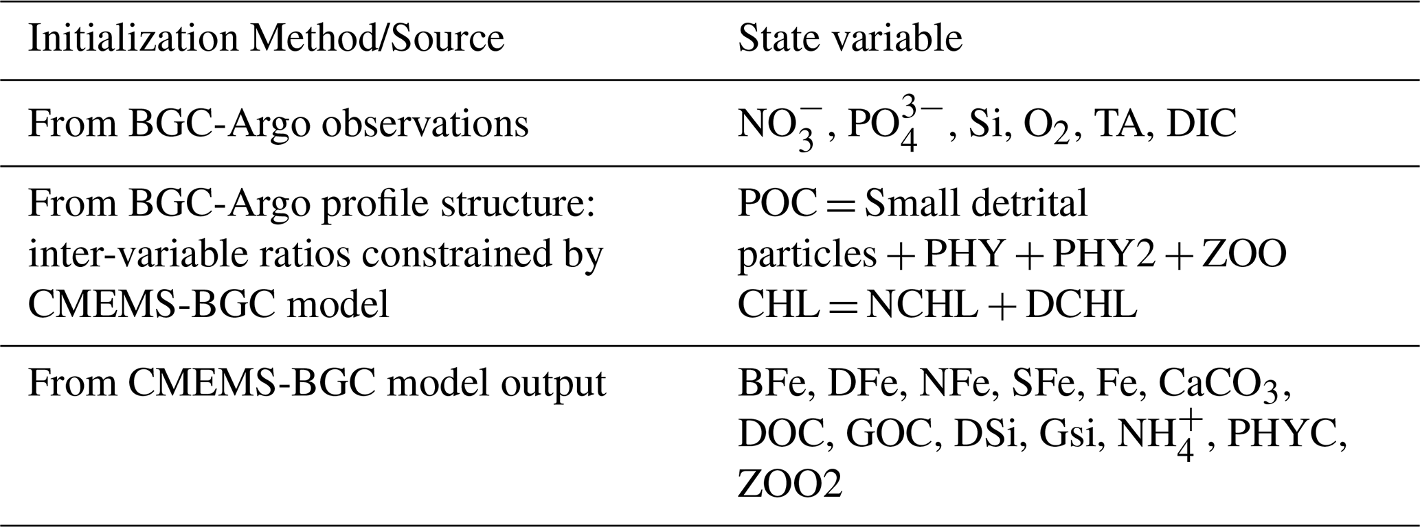
For variables not directly measured but inferred from float data, initial values were taken from the CANYON-B/CONTENT neural network products (pseudo-observations). Finally, initial conditions for any remaining unobserved variables were prescribed from the CMEMS-BGC analysis.

2.4.2 3D Global configuration

A global NEMO-PISCES configuration is run to estimate the representativeness error associated with unresolved three-dimensional processes in the 1D framework. To ensure methodological consistency, the global system uses the same NEMO-PISCES 4.2 code base as the 1D configuration, but with the biogeochemistry running online with the physics. The model grid has a horizontal resolution of $\mathrm{1}/\mathrm{4}$° and 75 vertical levels. The simulation covers the period 2010–2022 and is forced with ERA5 atmospheric reanalysis (Brodeau et al., 2010; Hersbach et al., 2020), complemented by a correction of a terrestrial heat-flux (Lucazeau, 2019). We refer to this experiment as the “3D-Free” simulation, which is a fully free-running integration without assimilation of physical or biogeochemical data.

2.4.3 3D IBI Regional Configuration

To assess the transferability of the optimized parameters in a fully three-dimensional framework, we used the IBI (Iberian–Biscay–Irish) regional system, which is based on the NEMO ocean engine coupled with PISCES, implemented at a horizontal resolution of $\mathrm{1}/\mathrm{36}$° (approximately 2–3 km) with 50 vertical levels and enhanced resolution near the surface. Two simulations were performed:

• i.

  REF: using the default PISCES parameter values.

• ii.

  OPTI: using the best-member parameter set from the All-Parameters optimization.

Both simulations span January 2017 to December 2019. Initial conditions for the biogeochemical variables were obtained from the CMEMS-BGC analysis, while physical variables (temperature, salinity, currents) were initialized from the CMEMS-PHYS analysis. Atmospheric forcing was provided by ECMWF at hourly temporal resolution. Model outputs were saved as daily averages.

3 Method

3.1 Metrics for sensitivity analysis and parameter optimization

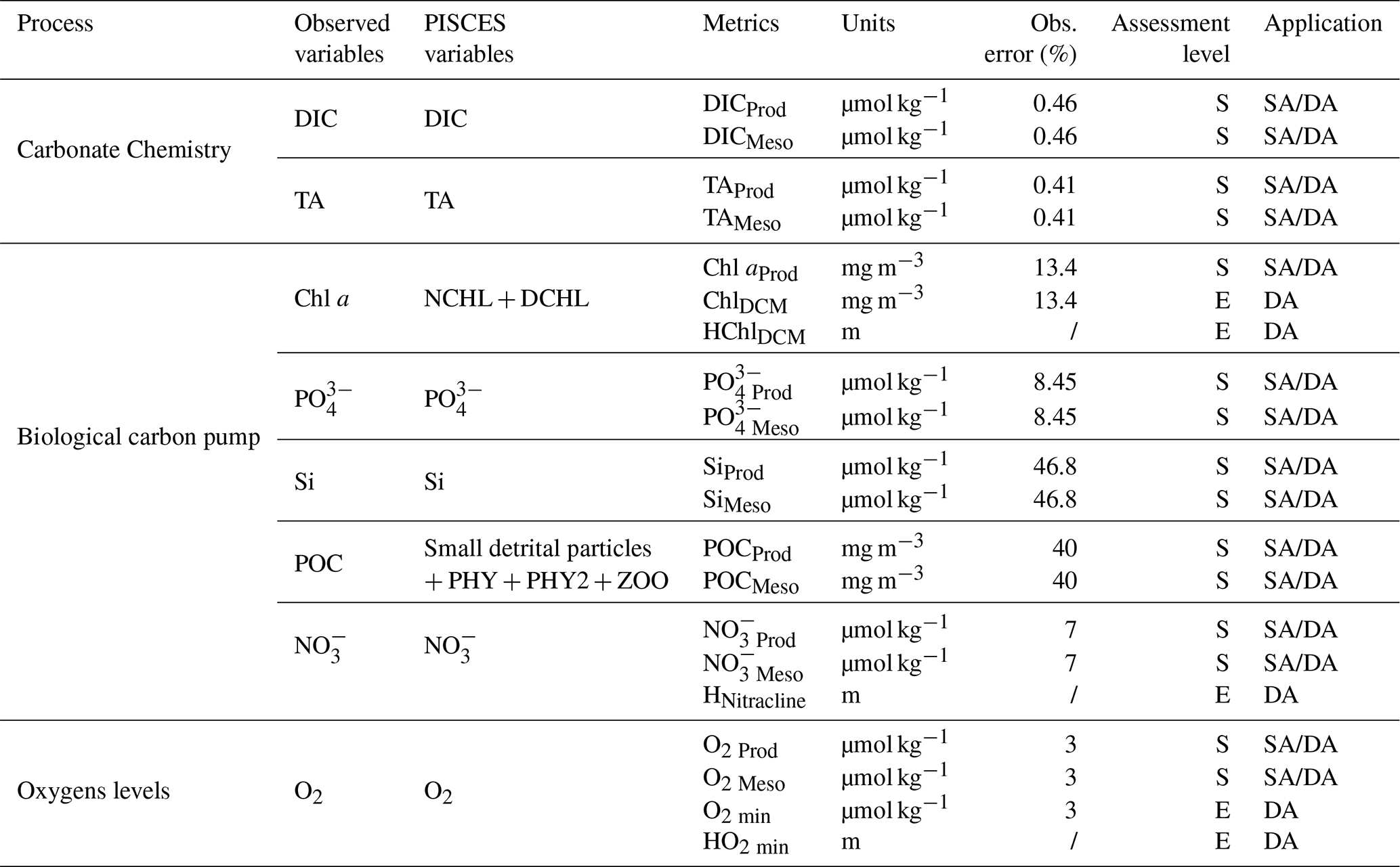
We define twenty observational metrics – layer-mean concentrations and vertical-structure diagnostics – derived from eight biogeochemical tracers measured or inferred from the BGC-Argo float (Mignot et al., 2023). These metrics serve as individual targets for the sensitivity analysis and optimization. Within the iIS framework, they enter the observation likelihood function, which determines the weight of each ensemble member based on how well it reproduces the observations across all 20 metrics simultaneously, accounting for the observation errors associated with each metric (Sect. 3.5). The prior parameter distributions are uniform, with bounds and inter-parameter constraints defined in consultation with the PISCES model developer (Sect. 3.4; Table S1). A concise description of all twenty metrics is provided in Table 2. Each layer-averaged metric is computed within two depth domains – the productive layer and the mesopelagic layer – using both BGC-Argo observations and the 1D model output. The following subsections detail the four steps required to calculate and compare these metrics: (1) the definition of the vertical layers used for analysis; (2) the calculation of layer-mean concentrations; (3) the diagnosis of emergent vertical features; and (4) the spatiotemporal interpolation procedure used to ensure a consistent comparison.

Table 2 Metrics used for sensitivity analysis (SA) and data assimilation (DA), showing the correspondence between observations and PISCES model variables. Only metrics designated as state variables (S) were used for the SA. Key: S = State variable; E = Emergent property.

3.1.1 Layer definitions and depth diagnostics

For our analysis, we subdivide the water column into two biogeochemically distinct layers. The productive layer extends from the surface down to the deeper of either the mixed-layer depth (MLD) or Z_Euphotic. The mesopelagic layer spans from the base of the productive layer down to 1000 m. These layers are defined by the MLD and Z_Euphotic, which are determined as follows for both the model and observations.

The MLD is diagnosed as the shallowest depth where potential density exceeds its surface value by 0.03 kg m⁻³ (de Boyer Montégut et al., 2004). For the model, daily MLD is computed from the potential density profiles from the CMEMS-PHY analysis. For observations, MLD is calculated from BGC-Argo temperature and salinity profiles using the same density threshold.

The euphotic depth, the depth where 1 % of surface photosynthetically available radiation (PAR) persists, is taken directly from the model's internal radiation scheme. For observations, the 1 % PAR depth is calculated from satellite-derived diffuse-attenuation coefficients, as detailed in Sect. 2.2.

3.1.2 Layer-mean metrics

Following (Mignot et al., 2023), we calculate layer-mean concentrations for a suite of eight state variables. For seven of these – DIC, TA, O₂, NO${}_{\mathrm{3}}^{-}$, PO${}_{\mathrm{4}}^{\mathrm{3}-}$, Si, and POC – we compute the mean concentration in both the productive and mesopelagic layers. For Chl a, the metric is computed for the productive layer only, as this layer contains the vast majority of its biomass and variability. This procedure yields a total of fifteen layer-mean metrics (eight for the productive layer and seven for the mesopelagic). To account for their lognormal distribution, the Chl a and POC metrics were subsequently log₁₀-transformed.

It is important to note that while model state variables are initialized directly from observational profiles, the initial values of the layer-mean metrics can still differ between the model and the BGC-Argo data. This discrepancy arises because the layer boundaries are diagnosed independently for the model and the observations, which can result in slightly different layer depths. Consequently, integrating a tracer profile with a strong vertical gradient over these different depth ranges will produce different initial layer-averaged values

3.1.3 Emergent vertical-structure metrics

To constrain processes that depend on vertical structure rather than bulk averages, we include five additional metrics that diagnose the depth and magnitude of key biogeochemical features:

• DCM: We record both the depth of the DCM (H_DCM) and the Chl a concentration at that depth (Chl_DCM). The DCM is crucial for phytoplankton growth and nutrient cycling in low latitude environment.

• Nitracline Depth (H_nitracline): This is defined as the first depth where NO${}_{\mathrm{3}}^{-}$ exceeds 1 µmol kg⁻¹, a threshold corresponding to the upper limit of BGC-Argo nitrate accuracy (Johnson et al., 2017; Mignot et al., 2019, 2023). This metric captures surface nitrate limitation, a key factor controlling primary production (Cermeño et al., 2008; Bendtsen et al., 2023)

• Oxygen Minimum: We identify both the depth of the minimum oxygen concentration ($H_{{\mathrm{O}}_{\mathrm{2}\min }}$) and the corresponding oxygen value (O_2 min). These quantities serve as proxies for mesopelagic remineralization intensity and ventilation (Stramma et al., 2008; Schmidtko et al., 2017).

3.1.4 Interpolation procedure

Before computing any metrics, both the simulated data and the float observations are processed and interpolated onto a common spatio-temporal grid. This procedure involves two steps. First, all vertical profiles are linearly interpolated onto a uniform 1 m vertical grid from the surface to 1000 m, from which each averaged metric within the productive and mesopelagic layers is then computed. Second, we address the irregular sampling of the float by linearly interpolating the observations to create a regular 5-day time series. Although the model provides daily outputs, we interpolate the time series of each metrics onto this same 5 d grid to ensure a direct, point-for-point comparison with the regularized observations. Finally, to reduce short-term variability and better highlight seasonal dynamics, a 6-point moving average is applied to smooth each metric's time series.

3.2 Parameter optimization method: Iterative Importance Sampling

This section describes the parameter optimization method. The central idea is to draw a large ensemble of model simulations from broad prior parameter distributions, then iteratively reweight the ensemble so that parameter sets producing good agreement with the observations receive higher weight. After several iterations, the resulting weighted ensemble provides an approximation of the posterior distribution, from which parameter estimates, uncertainties, and correlations can be extracted. The mathematical formulation is detailed below; the Bayesian likelihood function that drives the reweighting is presented in the Supplementary Information (Eq. S14).

To quantify posterior parameter correlations, uncertainties, and the predictive spread for both assimilated and unassimilated variables, we adopt iIS, an optimization scheme built on a particle-filter assimilation framework. Particle filters, widely used in biogeochemical modelling for state and parameter estimation (Mattern et al., 2013), are gradient-free ensemble methods that assimilate observations into a population of particles – each a unique, evolving model state – thereby generating full probability distributions for states and parameters. This approach is well suited to the strong non-linearities and non-Gaussian errors characteristic of marine biogeochemistry (Ristic et al., 2004).

Iterative Importance Sampling is a technique for estimating a probability density function (PDF) using a weighted combination of samples drawn from a different, known PDF .(Raices Cruz et al., 2022). In this work, this concept is applied within the framework of Bayesian inference to estimate model parameters. More formally, the goal is to approximate the posterior PDF of the model state variables and parameters, conditioned on observational data.

The Bayesian framework provides an approach for calculating the posterior PDF using prior knowledge and observational evidence. According to Bayes' theorem, the posterior distribution can be expressed as a function of the prior distribution and the observational likelihood (Wikle et al., 2013):

$$\begin{array}{}\text{(2)}& p\left(\mathit{x}|\mathit{y}\right)={\displaystyle \frac{p\left(\mathit{y}|\mathit{x}\right)p\left(\mathit{x}\right)}{\int p\left(\mathit{y}|\mathit{x}\right)p\left(\mathit{x}\right)\mathrm{d}\mathit{x}}}\end{array}$$

where $\mathit{x}=\left(s,\mathit{\theta }\right)$ is a random vector containing model state variables (s) and model parameters (θ), y is the observation vector, p(y|x) is the likelihood of the observations given the model outcome and p(x) is the probability of the model state. Here, following van Leeuwen et al. (2019) the prior probability is represented by an ensemble of N particles as:

$$\begin{array}{}\text{(3)}& p\left(\mathit{x}\right)=\sum _{j=\mathrm{1}}^N{\displaystyle \frac{\mathrm{1}}{N}}\mathit{\delta }\left(\mathit{x}-{\mathit{x}}_j\right)\end{array}$$

where x_j represents the jth member of the ensemble, and  δ(x − x_j), is the Dirac delta function that evaluates to 1 if x=x_j and 0 otherwise. Equation (3) means that the probability density function is a weighted sum of the delta functions centered at each member of the ensemble, where each member has an equal weight of N⁻¹.

The algorithm described in this article makes use of a self-normalized importance sampling techniques to estimate the posterior p(x|y) using weighted samples of p(x). Importance sampling generally involves the use of an auxiliary PDF, called proposal density function, whose main objective is to restrict sampling to regions of the state space with high probability (Owen and Zhou, 2000). In our setting, we used the prior p(x) as the proposal density since there is no reasonable estimate of the posterior distribution of the parameters. In this case the weights of each particle j is simply calculated using the observation likelihood (van Leeuwen et al., 2019) :

$$\begin{array}{}\text{(4)}& {\mathit{\omega }}_j={\displaystyle \frac{p\left(\mathit{y}|{\mathit{x}}_j\right)}{{\sum }_{j=\mathrm{1}}^{N}p\left(\mathit{y}|{\mathit{x}}_j\right)}}\end{array}$$

The posterior is then written as a weighted combination of the prior states:

$$\begin{array}{}\text{(5)}& p\left(\mathit{x}|\mathit{y}\right)=\sum _{j=\mathrm{1}}^N{\mathit{\omega }}_j\mathit{\delta }\left(\mathit{x}-{\mathit{x}}_j\right)\end{array}$$

Estimating model parameters from observations of the state is challenging because we often lack reliable prior information about the parameter distributions, and the relationship between the state and the parameters is typically highly non-linear. Moreover, models generally exhibit biases, partly due to uncertainty in the parameters and partly because of structural deficiencies, which include necessary simplifications, incomplete knowledge of key processes, and uncertainties in their mathematical representation. In the context of importance sampling, the small magnitude of observational noise significantly reduces the probability of obtaining model trajectories with high likelihood, thereby amplifying the impact of model imperfections.

Consequently, plain Monte Carlo sampling would produce many samples with negligible weights, making the estimation inefficient. To address this, the proposed algorithm evaluates Eqs. (4) and (5) iteratively, modifying the likelihood p(y|x) to p(y|x)^α, where α is an inflation parameter. This parameter is dynamically adjusted based on the effective sample size (ESS) defined as Martino et al. (2017):

$$\begin{array}{}\text{(6)}& \mathrm{ESS}={\displaystyle \frac{\mathrm{1}}{{\sum }_{j=\mathrm{1}}^N{\mathit{\omega }}_j^{\mathrm{2}}}}\end{array}$$

At each iteration, both the prior and the likelihood function are updated. The goal of each step is to construct a more informative prior, which allows for a gradual reduction of the inflation parameter α. Importantly, α plays a critical role in preserving parameter diversity throughout the iterations. It can also be interpreted as an inflation factor accounting for unresolved dynamics, analogous to error inflation techniques commonly used in the data assimilation community (see, e.g., Minamide and Zhang, 2017; Ohishi et al., 2022).

The sampling procedure is designed to efficiently explore the high-dimensional parameter space while keeping computational costs manageable. Model parameter samples are first drawn using Sobol's sequence, a low-discrepancy Quasi-Monte Carlo method (Sobol' et al., 2011), implemented through the scipy.stats.qmc.Sobol function in the SciPy library (Virtanen et al., 2020). Low-discrepancy sampling ensures more uniform coverage of the parameter space and reduces the risk of missing key regions of variability (Renardy et al., 2021). This method requires the sample size (N) to be a power of two.

To balance computational expense with sampling density, a dynamic ensemble size is used. For the first iteration, which must sample the entire broad prior parameter space, a larger ensemble of N=8192 is used. In subsequent iterations, where the sampling is focused on a narrower region of interest, the ensemble size is reduced to N=2048 to lower the computational cost.

The model is then integrated with these parameter sets to generate an ensemble of trajectories. Self-normalized importance weights are computed using the adaptive inflation factor (α), which is adjusted to maintain an effective sample size (ESS) of at least 25 % of the current ensemble size. In the final iteration of the iIS algorithm, the resampling process retains the top-ranked particles corresponding to the ESS, which resulted in a final optimized ensemble of 512 members.

For emergent metrics related to depth ($H_{{\mathrm{O}}_{\mathrm{2}\min }}$, H_nitracline, and H_DCM), we apply a uniform error distribution around the observational values. In practice, if a model realization produces a value outside the specified error range for any of these metrics, it is assigned a weight of zero. Additionally, some observed variations in these depth metrics are not captured by any simulation in the ensemble. This is particularly true for variations in the depth of the oxygen minimum, which appear to be driven more by physical than biogeochemical processes. To account for this, an additional condition is introduced: If more than 25 % of the simulations fall outside the error range for a given observation, that observation is excluded from the analysis. This approach assumes that such observations are influenced by physical processes not well represented in the model. Finally, DCM are not present in all vertical profiles, resulting in discontinuities in the corresponding time series. By applying this method, simulations that produce an unobserved DCM, as well as those that fail to reproduce an observed one, are filtered out.

To ensure biologically realistic growth rates of mesozooplankton in the model ensemble, an additional constraint based on temperature-dependent physiological dynamics has been implemented. Specifically, building on the work of Huntley (1992) and using the temperature measured by float #5904479, the maximum generation time of mesozooplankton should not exceed 30 d. Accordingly, the minimum plausible accumulation rate was set to 0.01 d⁻¹. To prevent the regeneration of ensemble members yielding unrealistically low mesozooplankton accumulation rates, any member with a maximum accumulation rate below 0.01 d⁻¹was assigned a weight of zero and therefore excluded from subsequent resampling.

To approximate the posterior distribution p(x|y), a kernel density function (KDF) is fitted using the KernelDensity class from the sklearn.neighbors module of the scikit-learn library (Pedregosa et al., 2011). The top-ranked particles corresponding to the ESS are retained, while the remaining particles are resampled from the fitted KDF. All weights are reset to N⁻¹ for the next iteration, and the PISCES model is re-run for the newly resampled particles (Fig. 3).

Figure 3 Schematic overview of the different datasets used during the parameter optimization process, referred to as iterative Importance Sampling (iIS).

This procedure is repeated iteratively until the inflation factor α converges or a predefined maximum number of iterations is reached. The proposed algorithm can also be interpreted as an adaptative IS method, following the classification of Elvira and Martino (2021), due to the use of a new proposal distribution, here, the prior p(x), at each iteration.

3.3 Sobol' Indices

The purpose of the sensitivity analysis is to identify which of the 95 PISCES parameters have a measurable influence on the assimilated metrics, and to quantify whether this influence operates directly (first-order effect) or through interactions with other parameters (higher-order effects). This information is used to define two reduced parameter subsets for comparison with the full 95-parameter optimization. The following subsections describe the theoretical framework (Sect. 3.3.1), the quantities of interest used to measure parameter influence (Sect. 3.3.2), and the selection criterion applied to define the parameter subsets (Sect. 3.3.3)

3.3.1 Theoretical framework

Sensitivity analysis plays a key role in the calibration of marine biogeochemical models such as PISCES, as it identifies the parameters that most strongly influence model outputs. For the purpose of this study, 'influential parameters' are defined as those whose variation accounts for a significant portion of the model output variance. By highlighting these parameters, SA enables a targeted reduction of the parameter space, thereby decreasing the computational cost of optimization. Given the inherent complexity and nonlinearity of modelled biogeochemical processes, the choice of an appropriate SA method is particularly important. In this study, we use a global method based on first-order and total-order Sobol' indices (Sobol', 2001). This section outlines the theoretical background, implementation, and criteria used for parameter selection.

Global Sensitivity Analysis using Sobol' indices offers a robust framework for quantifying the contribution of individual input parameters and their interactions to the variance in model outputs. Unlike local sensitivity methods, Sobol' indices account for nonlinear effects and interactions across the entire parameter space. This makes them particularly well-suited for complex models like PISCES, which involves 95 parameters with potentially intricate dependencies (Prieur el al., 2019; Issan et al., 2023).

Sobol' indices are derived from a functional Analysis Of Variance (ANOVA) decomposition of a scalar Quantity of Interest (QoI) of the model output, denoted by Y, as follows:

$$\begin{array}{}\text{(7)}& \begin{array}{rl}Y& =f_{\mathrm{o}}+\sum _i{f}_i\left({\mathit{\theta }}_i\right)+\sum _{i<j}{f}_{ij}\left({\mathit{\theta }}_i,{\mathit{\theta }}_j\right)+\mathrm{\dots }\\ & +f_{\mathrm{1},\mathrm{2},\mathrm{\dots },d}\left({\mathit{\theta }}_{\mathrm{1}},{\mathit{\theta }}_{\mathrm{2}},\mathrm{\dots },{\mathit{\theta }}_d\right)\end{array}\end{array}$$

where f_o is the mean output, and each term f_i or f_ij represents contributions of individual parameters or their interactions. $\mathit{\theta }=\left({\mathit{\theta }}_{\mathrm{1}},{\mathit{\theta }}_{\mathrm{2}},\mathrm{\dots },{\mathit{\theta }}_d\right)$ is the parameter vector, and d is the number of parameters.

Sobol' indices distinguish between direct parameter effects and higher-order interactions. The first-order Sobol' index quantifies the proportion of output variance attributable to a single parameter while accounting for variations in all other inputs (Sobol', 2001). In contrast, the total-order index captures both the direct contribution of a parameter and all its interactions with other parameters, including second-order and higher-order dependencies, offering a comprehensive measure of its influence. For the sake of simplicity, first-order Sobol indices will be referred to as “Main effects”, and total-order Sobol indices as “Total effects” throughout this paper. The mathematical definitions of S_i and T_i are given in the Supplement (Eqs. S1–2).

A key step in implementing Sobol' analysis is the construction of input sampling matrices, which are used to generate different model simulations. Monte Carlo methods or quasi-random sampling techniques, such as Sobol' sequences, are commonly used to estimate these indices, requiring multiple model evaluations (Campolongo et al., 2000). Following the approach described by Issan et al. (2023), the process involves:

1. Generating a baseline matrix (A): A matrix where each row represents a parameter set sampled from its respective probability distribution. This matrix has dimension N×d, where N represents the number of samples per parameter and d the number of parameters studied.

2. Generating a perturbed matrix (B): A second independent sample matrix of the same size as A.

3. Constructing hybrid matrices (C): Matrix C is generated by replicating matrix (A) d times. In the ith copy, the ith line of B is replaced with the corresponding line from matrix A, denote as $\mathbf{A}(:,i)$. This procedure ensures that each parameter is individually perturbed while keeping all others unchanged.

   $$\begin{array}{}\text{(8)}& {\mathbf{C}}^{\left(i\right)}=\left[\begin{array}{ccc}& \mathbf{B}(:,\mathrm{1})& \\ & \mathrm{⋮}& \\ -& \mathbf{A}(:,i)& -\\ & \mathrm{⋮}& \\ & \mathbf{B}(:,d)& \end{array}\right]\in R^{N\times d},i=\mathrm{1},\mathrm{\dots },d\end{array}$$

In this study, both the first-order and total-order Sobol sensitivity indices are estimated for 95 PISCES model's parameters. Using Sobol's method, the total-order sensitivity can be estimated with $N\times (d+\mathrm{2})$ model evaluations. To ensure a robust estimation of the sensitivity indices, the parameter space must be sampled with a sufficiently large number of points (N). The sample size was chosen to be consistent with established practice for such high-dimensional models (Prieur et al., 2019; Issan et al., 2023). Therefore, N was set to 2¹⁴, as the Sobol' sequence sampling method is most efficient when the number of samples is a power of two. Additionally, the same parameter ranges as those defined during the initialization of the iIS (see Sect. 3.5) are imposed.

To perform sensitivity analysis efficiently, the Python Sensitivity Analysis Library (SALib) enables both parameter space sampling and the computation of first-order and total-order Sobol indices (Iwanaga et al., 2022). The sampling is conducted using the Sobol sequence, a quasi-random method with low discrepancy (Sobol', 2001).

3.3.2 Definition of the Quantity of Interest (QoI)

For each metric defined in Table 2, except for those describing emergent properties, two QoIs are computed. The first is the RMSE, which quantifies the discrepancy in amplitude between the modeled and observed metrics. The second is the temporal correlation between the modeled and observed metrics, intended to assess the sensitivity of the system's temporal dynamics to variations in the model parameters.

More precisely, for each metric M and ensemble member j, we compute the root-mean-square error between the simulated and observed time series, and the Pearson correlation coefficient between them (Eqs. S3–4 in the Supplement).

3.4 Parameter selection for optimization

The aim is to include in the iIS procedure only those parameters that have an impact on the assimilated metrics, and therefore only those parameters that can be significantly constrained by the metrics defined in Table 2. Parameters that do not significantly influence these metrics, either in terms of phenology or amplitude, are not perturbed. For such non-influential parameters, we assume that their reference values should be retained, as there is insufficient information to constrain their uncertainties.

To identify influential parameters, we select all parameters with a Sobol' sensitivity index (first-order or total-order; see Sect. 3.3 for details) greater than 0.02 for at least one quantity of interest (QoI), following the approach of Prieur et al. (2019). This filtering step yields a reduced parameter set, thereby lowering the dimensionality of the parameter uncertainty space.

3.5 Parameter perturbation

We have shown in Sect. 3.2 and 3.3 that both iIS and Sobol' sensitivity analysis require a prior estimate of the parameters' probability density functions. In practice, however, limited information about these parameters is available in the literature; most often, only plausible value ranges are reported (Denman, 2003).

Given this lack of detailed prior knowledge, we assume uniform distributions. This choice reflects a non-informative prior assumption, treating all values within the specified interval as equally likely. It provides a conservative starting point for inference, minimizing subjective bias.

To account for the possibility that fitting the ensemble of assimilated metrics may require the model to reach a substantially different equilibrium state, we define broad perturbation intervals, ranging from one-hundredth to twice the reference values. To ensure physical consistency, certain parameters are subject to additional constraints to prevent unrealistic phenomena such as the artificial generation or loss of matter for example (Table S1 in the Supplement).

3.6 Observation errors

In the Sect. 3.2 each particle is weighted using the observation likelihood. As noted by van Leeuwen et al. (2019), the likelihood function p(y|x) quantifies the probability of obtaining the observation y assuming that x represents the true state. Given that observations are modeled as $\mathit{y}=H\left(\mathit{x}\right)+\mathit{ϵ}$, with H a possibly non-linear observation operator mapping from the model state to the observation space and ϵ a random noise following a known distribution, the likelihood becomes a function of the discrepancy between the observed and model-predicted values, shifted by the noise distribution p_ϵ :

$$\begin{array}{}\text{(9)}& p\left(\mathit{y}|\mathit{x}\right)=p_{\mathit{\epsilon }}(\mathit{y}-H(\mathit{x}\left)\right)\end{array}$$

Therefore, accurately estimating observational errors is crucial, as these errors directly influence the weighting of particles in the importance sampling procedure. We consider two main sources of observational error: measurement error and representativity error. Measurement error accounts for uncertainties in mapping from the model state to the observation space. This includes uncertainties associated with the observation operator (H) itself, the instrumental precision of direct sensor measurements, and the inferred uncertainty of variables derived from neural networks (e.g., CANYON-B). Representativity error, in contrast, arises from discrepancies between what the 1D model can simulate and the finer-scale or unresolved 3D features present in the observations. The explicit form of the likelihood function is given in the Supplementary Information (Eq. S14).

The observation error ϵ is assumed to follow a Gaussian distribution for most metrics. However, for metrics related to the depth of the nitracline, the DCM, and the depth of the oxygen minimum, a uniform distribution is used. Within the iIS procedure, this choice effectively excludes particles that produce unrealistic values for these depth-related variables.

3.7 Measurement errors

The observation likelihood in iIS requires an estimate of the measurement uncertainty for each metric. We used four distinct methods to compute these errors, each tailored to a specific group of metrics. The resulting observation errors, expressed in percentages, are shown for each metric in Table 2.

3.7.1 Direct observations (Chl a, O₂, NO${}_{\mathrm{3}}^{-}$)

For variables directly measured by BGC-Argo (Chl a, O₂, NO${}_{\mathrm{3}}^{-}$), we defined the measurement error based on the mean RMSE values reported in Mignot et al. (2019). That study calculated the RMSE between float observations and co-located, ship-based measurements. To convert these absolute RMSE values into the relative percentage errors required for our study, we normalized them by the average of the same ship-based reference dataset used in Mignot et al. (2019). For this normalization, we used a robust mean, calculated after excluding the top and bottom 5 % of the reference data to reduce the influence of outliers.

3.7.2 Particulate Organic Carbon

For the POC concentrations derived from particulate backscatter, we adopt a fixed relative measurement error of 40 %. This choice is based on the error model of Johnson et al. (2017), which recommends using the greater of an absolute error of 35 mg C m⁻³ or a relative error of 20 %. For our study region, the mean observed POC concentration in the productive layer is approximately 79 mg C m⁻³ . At this concentration, the absolute error threshold of 35 mg C m⁻³ is equivalent to a relative error of ∼ 44 % (i.e., $\mathrm{35}/\mathrm{79}$). Since this is greater than the 20 % relative error threshold, it becomes the dominant error source. We therefore adopt a rounded, conservative value of 40 % for the POC measurement error.

3.7.3 Error representation for log-transformed metrics

The metrics for Chl a and POC concentration are log₁₀-transformed to account for their lognormal distribution. Consequently, their respective relative percentage errors are converted into a fixed, additive error in log-space. This error is calculated using a first-order error propagation formula; (error % $/$ 100) $/$ ln(10).

3.7.4 Uncertainty of Neural Network-Derived Variables

The measurement error for variables derived from the CANYON-B and CONTENT neural networks (i.e., PO${}_{\mathrm{4}}^{\mathrm{3}-}$, Si, TA, and DIC) was estimated by quantifying and combining two main sources of uncertainty: the propagated uncertainty from input oxygen measurements, and the intrinsic uncertainty of the network algorithms themselves.

This analysis was performed on a computationally feasible subset of the data (1313 points, selected by taking one of every 20 points from the full profiles). For each of these data points, we first calculated a total measurement error. The propagated uncertainty was quantified via a Monte Carlo experiment in which 300 perturbed oxygen values (assuming a 3 % input error) were passed through the networks to find the standard deviation of the outputs. This was combined in quadrature with the intrinsic uncertainty, which is a direct output of the neural networks.

This process yielded a set of 1313 total error estimates. To derive a single, robust value for each variable, we then calculated the mean of these 1313 estimates after excluding the top and bottom 5 % as outliers. Finally, this mean total error was normalized by the mean of the corresponding 1313 variable observations to yield the final percentage error reported in Table 2.

3.7.5 Uncertainty in depth-based metrics

For depth-based metrics (H_DCM, H_nitracline, $H_{{\mathrm{O}}_{\mathrm{2}\min }}$), we used a gradient-based approach. For each individual profile, we first estimated a depth uncertainty by dividing the known concentration error of the relevant variable (e.g., Chl a error for H_DCM) by the local vertical concentration gradient at that feature's depth. This procedure yielded a time series of individual depth error estimates for each metric.

To derive a single, robust error value for the entire time series, we used the interquartile range (IQR). After calculating all the individual depth errors, the final representative uncertainty (in meters) was defined as the width of the interquartile range (i.e., the 75th percentile minus the 25th percentile) of these estimates. This method was chosen over a simple mean or median because the distribution of depth errors was highly skewed, and the IQR provided a more stable and representative measure of the typical uncertainty, avoiding inflation from extreme outliers.

BGC-Argo floats typically do not sample the top few meters of the water column, creating an “unseen” surface layer. If a feature, was detected at the shallowest point of a profile, it is impossible to know if the true maximum was at that depth or shallower, within the unsampled layer. To account for this ambiguity, we introduced an additional uncertainty term in these specific cases. This term was set equal to the depth of the shallowest observation itself, effectively representing the possibility that the true feature depth could be anywhere between the surface and the first measurement. This additional term was combined in quadrature with the gradient-based depth error.

3.8 Representativity errors

Using a 1D model to represent a 3D ocean introduces a “representativity error” due to neglected 3D physical processes. To account for this, the cost function used in our assimilation combines observational errors with this representativeness term. Including this error limits the extent to which the optimization compensates for missing physics, yielding a more reliable calibration. The magnitude of this error was quantified at each time step as the absolute difference between the value from the full “3D-Free” simulation (sampled along the float's trajectory) and the value from the corresponding 1D simulation (“1D-Free”, initialized and forced with the same 3D fields).

This time-dependent representativity error is then added in quadrature to the measurement error at each corresponding time step, creating the total observational error used in the likelihood calculation. This approach allows for greater uncertainty during periods when the 1D assumption is weakest, prevents overconfidence in observational constraints, and reduces the risk that the parameter optimization compensates for missing physics with unrealistic parameter values.

3.9 Assessment of Neglected Error Sources

In addition to measurement and representativity errors, we also evaluated two other potential sources of uncertainty: (i) error covariances among the observed and derived variables, and (ii) grid discretization errors.

First, to assess the impact of error covariances, we estimated the full error covariance matrix for the observation vector. We propagated a 3 % perturbation in the input oxygen observations through the CANYON-B and CONTENT algorithms to quantify the covariance terms both among the network-derived variables (e.g., DIC, TA) and between those variables and the uncertain input (O₂). A comparative analysis demonstrated that including these off-diagonal covariance terms in the likelihood calculation had a negligible effect on the final results; the RMSE between the optimized solution and the observations changed by less than 2 %.

Second, we assessed the impact of grid discretization error. This error arises because the 1D model is forced by a single grid point from the $\mathrm{1}/\mathrm{4}$° physical model, while the true float position varies within that grid cell. To test the sensitivity to this choice, we ran an ensemble of 1D simulations where each member was forced by a different, randomly selected $\mathrm{1}/\mathrm{12}$° sub-grid point from within the same $\mathrm{1}/\mathrm{4}$° grid cell. By comparing simulations with identical parameters but different physical forcing, we could quantify the influence of this sub-grid variability. The analysis indicated that the resulting grid-induced differences were minor compared to measurement and representativity errors; including this physical uncertainty in the optimization process changed the final RMSE between the optimized solution and the observations by less than 2 %.

Given the significant computational cost required to quantify these two error sources and their minor impact on the results, both were excluded from our final error budget.

3.10 Framework for Performance Evaluation

We evaluate the effectiveness of the three optimization strategies using statistical criteria that assess three key aspects of performance:

• Goodness of fit: The improvement in skill against the assimilated data is quantified using the Normalized Root Mean Square Error (NRMSE).

• Ensemble evaluation: The solution's performance against independent data is tested using the reduced centred random variable metric (RCRV).

• Parameter Constraints: The impact on the model parameters is assessed by measuring the reduction in their posterior uncertainty via the Highest Density Interval (HDI) and by calculating the correlations among them to test for independence.

The Normalised Root Mean Square Error (NRMSE) is our primary metric for quantifying the misfit between simulated and observed metrics. We calculate two versions for each metric M: one for the single best ensemble member and one for the weighted-mean ensemble. The NRMSE normalises the RMSE by the total observation error $\mathit{\epsilon }{\mathit{\epsilon }}_t^{\mathrm{M}}$ (measurement and representativity errors combined in quadrature) so that a value of ∼ 1 indicates model-data misfit comparable to the expected observation error, while values less than 1 indicate a good fit (Eqs. S5–8 in the Supplement). The performance of the optimized simulations is then evaluated by comparing their NRMSE values to that of the reference simulation with default PISCES parameters (hereafter REF). The optimized simulations are referred to as OPTI. For both the best-member and ensemble NRMSE, the relative change in performance is quantified as Δ%NRMSE = (NRMSE_OPTI− NRMSE_REF) $/$ NRMSE_REF×100 %, so that negative values indicate improvement

To assess the performance of the optimized ensembles against independent observations, we use the Reduced Centred Random Variable (RCRV). At each time step, the RCRV normalises the residual between the weighted ensemble mean and the observation by the total uncertainty, combining observation error and ensemble spread in quadrature (Eqs. S9–12 in the Supplement). The time-mean RCRV (bias) measures systematic error: values near zero indicate an unbiased ensemble. The standard deviation of the RCRV (dispersion) measures calibration: a value of 1.0 indicates a perfectly calibrated ensemble, values below 1.0 indicate a conservative (over-dispersive) ensemble, and values above 1.0 indicate an overconfident one.

We quantify the reduction in parameter uncertainty by the percentage change in the 67 % Highest Density Interval (HDI) between the prior and posterior distributions (Eq. S13 in the Supplementary Information). The HDI represents the narrowest credible interval containing 67 % of the probability mass. Negative values indicate that the posterior is narrower than the prior, i.e., the observations have reduced parameter uncertainty.

Finally, we calculate the pairwise correlation coefficients between all optimized parameters using the 512 best-weighted ensemble members from each strategy. This analysis tests whether the assimilation framework successfully found an independent solution for each parameter, a key indicator of a well-constrained system.

3.11 Three-dimensional validation framework

For the surface chlorophyll a validation against MOBTAC, we adopt the five regional boxes defined by Gutknecht et al. (2019) in their formal skill assessment of the CMEMS IBI biogeochemical system (Fig. 10b): Box 1 (Celtic Sea/Rockall Trough), Box 2 (Canary/Madeira region), Box 3 (Bay of Biscay), Box 4 (Gulf of Lion), and Box 5 (Balearic Sea). Using the same geographical framework ensures direct comparability with the established IBI validation protocol.

These boxes are, however, too small to yield robust statistics for the subsurface BGC-Argo validation, where float coverage is much sparser – particularly in the North Atlantic, which concentrates only 10 %–15 % of the matched profiles. The IBI domain was therefore divided into three broader sub-regions for the BGC-Argo assessment (Fig. 10b): (i) Northern basin (20° W–17° E, 48–65° N), (ii) Iberian Atlantic (20–5° W, 26–48° N), and (iii) Mediterranean and Bay of Biscay (5° W–17° E, 26–48° N). For the aggregated analysis presented in Sect. 5, the Northern and Iberian Atlantic basins are further combined into a single “North Atlantic” region.

The technical details of the model–observation colocation procedure and the adaptation of the NRMSE metric for the 3D assessment are provided in the Supplementary Information (Sect. S2). In brief, subsurface BGC-Argo profiles are matched to the IBI model in space, depth, and time over the 0–500 m range, with model values interpolated horizontally, vertically, and temporally to each float observation. Surface chlorophyll a is compared on the MOBTAC 0.25° grid using monthly means in log₁₀-transformed space, displayed on Taylor diagrams. Model performance is assessed using the same NRMSE framework as in Sect. 3.9, with two differences: the representativity error term is omitted (since the 3D model resolves the processes it was designed to account for), and the observation uncertainty uses the point-by-point error field associated with each BGC-Argo measurement rather than the propagated Monte Carlo estimates. The Δ%NRMSE is computed as defined in Sect. 3.9. When both NRMSE values fall below unity, a positive Δ%NRMSE does not constitute a meaningful degradation, since both simulations already reproduce observations within their associated uncertainties.

4 Results

4.1 Global Sensitivity Analysis

The GSA revealed that the parameter controlling organic matter recycling (e.g., the half-saturation constant for DOC remineralization, K_DOC) exerted the strongest first-order influence, primarily through its impact on mesopelagic concentrations of DIC, nitrate, phosphate, and dissolved oxygen (Fig. 4a). This parameter, however affected only a limited subset of metrics. In contrast, the phytoplankton light response (e.g., the P-I slope for nanophytoplankton, α^Nano) showed significant effects on almost all state variables, including those in the mesopelagic layer. Zooplankton parameters also emerged as important drivers, particularly those related to grazing and prey preference (e.g., the microzooplankton preference for nanophytoplankton, $P_{\mathrm{Nano}}^{\mathrm{MicroZoo}}$, and the half-saturation constant for microzooplankton grazing, $K_{\mathrm{G}}^{\mathrm{MicroZoo}}$).

The total-order analysis demonstrated that many of the most influential parameters, especially for zooplankton, acted primarily through interactions rather than direct effects (Fig. 4b). For instance, the non-assimilated fractions of nanophytoplankton consumed by microzooplankton (σ^MicroZoo) and mesozooplankton (σ^MesoZoo) were ranked as the first and second most sensitive parameters overall, despite having only weak first-order effects (Fig. 4a). In contrast, K_DOC displayed similar sensitivity in both the first-order and total-order analyses, suggesting its influence is largely independent of parameter interactions (Fig. 4a). When accounting for interactions, seven parameters had significant impacts on all model metrics (α^Nano, $P_{\mathrm{Nano}}^{\mathrm{MicroZoo}}$, $K_{\mathrm{G}}^{\mathrm{MicroZoo}}$, $K_{\mathrm{G}}^{\mathrm{MesoZoo}}$, ${\mathit{\theta }}_{\mathrm{Max}}^{\mathrm{Fe}\mathrm{Nano}}$, $G_{\mathrm{m}}^{\mathrm{MicroZoo}}$, $G_{\mathrm{m}}^{\mathrm{MesoZoo}}$). These correspond to parameters of microzooplankton, mesozooplankton and nanophytoplankton, highlighting their central role in biogeochemical dynamics (Fig. 4b).

By contrast, nine parameters related to processes irrelevant to the float's open-ocean location – such as the half-saturation constant for anoxia, coastal iron release, and iron concentration in sea ice – showed no measurable influence.

Figure 4 First-order and Total-order Sobol sensitivity indices of the parameters across the assimilated metrics. Sensitivity is defined as the maximum between the index estimated via RMSE and that estimated via correlation. Only parameters with a sensitivity index greater than 0.02 for at least one metric are shown. Panel (a) displays the first-order Sobol indices, while panel (b) shows the total-order Sobol indices. Grey cells indicate a sensitivity index below 0.02, which is considered non-significant in this study. Parameters are ranked in descending order based on their maximum Sobol indices. They are grouped according to the same categories defined in the PISCES model. Metrics defined as emerging properties are not used in this study.

4.2 Productive Layer Skill

All three parameter optimization strategies improved the simulation of the productive-layer seasonal cycle, correcting biases present in REF. The three optimized ensembles – All-parameters (Fig. 5), Total effects (Fig. S2), and Main effects (Fig. S5) – produce nearly identical corrections. In all cases, the ensembles capture the magnitude and timing of the spring phytoplankton bloom, as indicated by Chl a concentrations (Fig. 5a). This improvement is reflected across related variables: the model reproduces the observed seasonal drawdown of NO${}_{\mathrm{3}}^{-}$, PO${}_{\mathrm{4}}^{\mathrm{3}-}$ and DIC, and the concentration of Chl a and POC aligns with float data (Fig. 5a–d, f).

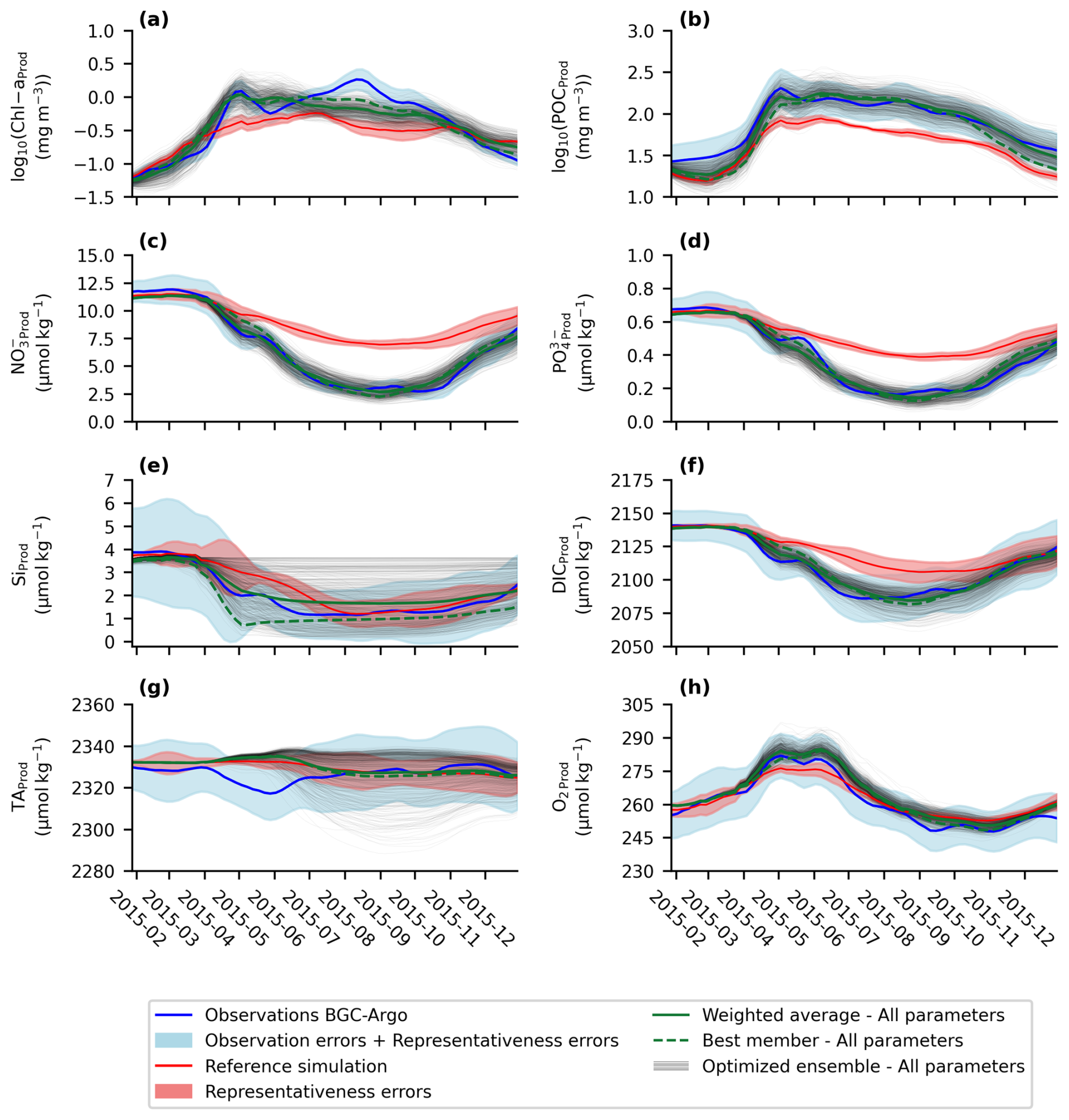
Figure 5 Seasonal cycle of assimilated metrics in the productive layer. Panels show: (a) log₁₀(Chl a_Prod), (b) log₁₀(POC_Prod), (c) NO${}_{\mathrm{3}\mathrm{Prod}}^{-}$, (d) PO${}_{\mathrm{4}\mathrm{Prod}}^{\mathrm{3}-}$, (e) Si_Prod, (f) DIC_Prod, (g) TA_Prod, and (h) O_2 Prod. The blue curve represents observations from BGC-Argo float #5904479, with the blue shading indicating the combined observations and representativity errors. The red curve corresponds REF from PISCES-1D, with the red shading representing representativity errors. Green line indicate the weighted means of the ensemble optimized using All parameters of the PISCES model. The black curves represent the ensemble of selected members obtained by optimizing all parameters of the PISCES model. A six-point moving average was applied to all time series to smooth short-term fluctuations.

Figure 6 Seasonal cycle of assimilated metrics in the mesopelagic layer. Panels show: (a) log₁₀(POC_Meso) (b) NO${}_{\mathrm{3}\mathrm{Meso}}^{-}$, (c) PO${}_{\mathrm{4}\mathrm{Meso}}^{\mathrm{3}-}$, (d) Si_Meso, (e) DIC_Meso, (f) TA_Meso, and (g) O_2 Meso. The blue curve represents observations from BGC-Argo float #5904479, with the blue shading indicating the combined observations and representativity errors. The red curve corresponds to REF from PISCES-1D, with the red shading representing representativity errors. Green line indicate the weighted means of the ensemble optimized using All parameters of the PISCES model. The black curves represent the ensemble of selected members obtained by optimizing all parameters of the PISCES model. A six-point moving average was applied to all time series to smooth short-term fluctuations.

Figure 7 Seasonal cycle of assimilated emerging metrics. Panels show: (a) O_2 min, (b) H_Nitracline, (c) HO_2 min. Chl_DCM and H_DCM are not shown, as there were not enough DCM observations to reconstruct these metrics. The blue curve represents observations from BGC-Argo float #5904479, with the blue shading indicating the combined observations and representativity errors. The red curve corresponds to REF from PISCES-1D, with the red shading representing representativity errors. Green line indicate the weighted means of the ensemble optimized using All parameters of the PISCES model. The black curves represent the ensemble of selected members obtained by optimizing all parameters of the PISCES model. A six-point moving average was applied to all time series to smooth short-term fluctuations.

These visual improvements are confirmed by a large and statistically robust reduction in the model-data misfit (Table 3a). For the assimilated float, the three strategies achieved a comparable median NRMSE reduction across the eight productive-layer metrics: −55.6 % (± 36.1 %) for Main effects, −54.2 % (± 24.2 %) for Total effects, and −53.6 % (± 29.9 %) for All-parameters. In all cases, the median improvement is larger than the associated interquartile uncertainty, indicating an enhancement of the goodness of fit. Given the small sample size (n=8 metrics), we used a non-parametric Kruskal-Wallis H-test to formally compare the distributions of NRMSE reductions. For the weighted-mean ensembles, the test confirmed that there is no statistically significant difference among the three strategies (p=0.99). This similarity in performance demonstrates that while a small subset of highly sensitive parameters drives most of the improvement, perturbing all 95 parameters achieves the same skill.

Table 3 Normalized Root Mean Square Error (NRMSE) across the metrics, with IQR/2 shown in parentheses. RMSE values are normalized by the combined observational and representativity errors. Percentage improvements are calculated as the relative difference between the NRMSE of OPTI and REF. Negative values indicate improved performance. Results are presented for the assimilated float (#5904479). Columns compare REF against three parameter selection strategies. “Main effects” and “Total effects” refer to parameter selections based on first-order and total-order Sobol indices, respectively, while “All Parameters” corresponds to optimization using the full parameter set. For each method, “Best” denotes the simulation with the highest weight, and “Ensemble” represents the weighted mean across all ensemble members. Values represent the median percentage improvement in metrics related to the productive layer (a), and for all remaining metrics (b). Note that metrics related to the DCM were excluded due to the lack of long-term observational data for this metrics. Uncertainty on the median improvement is estimated using half the interquartile range of the percentage improvements across the metrics.

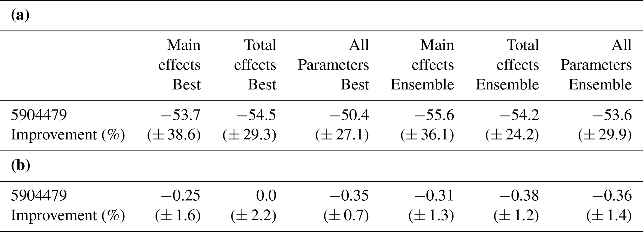
The median NRMSE of the weighted-mean ensemble for each strategy was comparable to that of its single best-performing member (Table 3a). However, the ensemble weighted mean (solid lines, Fig. 5) consistently provided a smoother and more physically plausible representation of the seasonal cycle than any individual “best” member simulation (dashed lines), which is a known advantage of the ensemble approach (Germineaud et al., 2019). Regarding the parameters themselves, while the overall posterior distributions were largely similar across the three strategies, the specific values for the single best-performing member of each strategy show notable differences. These parameter sets are provided in Table S1 as a concrete and reusable outcome for future studies.

4.3 Deeper properties skill

In contrast to the productive layer, the optimized ensembles closely resemble REF for the mesopelagic layer and for emergent vertical properties (Figs. 6, 7 and S3, S4, S6, S7). For most deeper metrics, such as nutrients, oxygen and carbonate chemistry, the optimized ensembles remain nearly indistinguishable from REF. This outcome can be attributed to several factors: REF already simulated these variables with reasonable skill, leaving little mean bias for the optimization to correct (e.g., Fig. 7a, c); mesopelagic properties have long adjustment timescales, making a one-year assimilation period insufficient to induce substantial changes; and the 1D model configuration neglects the deep advective processes that drive much of the variability in the ocean interior.

Mesopelagic POC is an exception. Its dynamics are forced by particle export from the surface, giving it a shorter response timescale than the other deep tracers. For this variable, the optimization mitigated a bias present in the reference run, improving the simulation skill (Fig. 6a).

For these deeper properties, the optimization therefore did not correct large mean-state biases, but penalized parameter sets that drifted away from the observations. For instance, the assimilation penalized any parameter set that produced an unrealistic nitracline depth or oxygen minimum, ensuring the optimized ensembles remained consistent with the float data throughout the simulation period.

This limited overall impact is confirmed by the error statistics. For the seven non-productive-layer metrics, the median NRMSE improvements for the weighted-mean ensembles were negligible: −0.31 % (± 1.3 %) for Main effects, −0.38 % (± 1.2 %) for Total effects, and −0.36 % (± 1.4 %) for All-parameters (Table 3b). The associated uncertainty (IQR) for each strategy is several times larger than the median improvement, and a Kruskal-Wallis H-test confirmed that the differences among the strategies are not statistically significant (p=0.99). These results suggest that while the framework can constrain specific, well-observed features at any depth, the one-year assimilation period is insufficient to correct for potential systemic biases in slower, deeper biogeochemical processes.

As with the productive layer, the median NRMSE for the weighted-mean ensemble of each strategy was statistically indistinguishable from that of its corresponding single “best” member (Table 3b). For these deeper properties, where model-data misfits are often smaller and less dynamic, the visual difference between the smoother ensemble mean and the more variable best-member simulation is less pronounced than in the surface layer, but the principle remains that the ensemble mean provides a more robust estimate.

4.4 Uncertainty in Unassimilated Variables

While all three optimization strategies showed comparable skill against assimilated data, their performance diverged when estimating the predictive uncertainty for unassimilated variables (Fig. 8). The Main effects ensemble, which perturbed only 29 parameters, produced the smallest uncertainty spread, with a median standard deviation of 0.17 (± 0.16) relative to the seasonal cycle of the unobserved metrics. In contrast, the Total effects (66 parameters) and All-parameters (95 parameters) ensembles produced larger spreads, with median values of 0.29 (± 0.21) and 0.27 (± 0.26), respectively.

Figure 8 Standard deviation (unitless) of the ensemble optimized using different parameter selection strategies, normalized by the variability of the seasonal cycle in REF. The X-axis indicates unassimilated state variables as well as two derived outputs : carbon export at 100 m depth and integrated net primary production (INTPP). Results are shown for the three parameter selection strategies : “Main effects (N=29)”, `Total effects (N=66)” and “All parameters”. Each point corresponds to a specific metric, with dashed lines indicating the median value.

Formally, a Kruskal-Wallis H-test on these distributions of uncertainty spreads does not indicate a statistically significant difference between the three strategies at the α=0.05 level (p = 0.26). The difference in median spread is nonetheless a direct consequence of where each variable's uncertainty comes from. For the assimilated variables, the observations constrain the predictions: parameter sets that fit the data poorly are given little weight, so all three strategies converge on a similar, narrow spread regardless of how many parameters were free to vary – hence their comparable skill. The unassimilated variables carry no such constraint, so their predictive spread reflects only the parametric uncertainty that each strategy propagates. The Main effects strategy holds most parameters – including many that the GSA showed exert influence mainly through interactions – fixed at their default values, and so removes part of that uncertainty by assumption rather than because the data exclude it. The resulting narrow spread is therefore an underestimate of the model's parametric uncertainty.

Conversely, the Total effects and All-parameters strategies allow a larger set of influential parameters to vary, propagating their uncertainty into the ensemble spread. The wider predictive spreads they produce reflect the propagated parametric uncertainty rather than a degradation in model skill. Therefore, we conclude that while any of the strategies can produce a skillful “best-guess” simulation, approaches that perturb more parameters provide a fuller quantification of predictive uncertainty, which is required for forecasting and climate-projection applications.

4.5 Parameter Uncertainty and Correlation

Assimilating the BGC-Argo data reduced parameter uncertainty unevenly across the 95 parameters, as measured by the percentage reduction in the 67 % HDI of each parameter distribution (Table 4). The reduction was concentrated in the parameters with the highest Sobol indices. This targeted nature is most evident in the All-parameters experiment. In this run, the median HDI reduction showed a clear cascade based on parameter sensitivity: the reduction was greatest for the Main effects subset (−27.4 %), smaller for the broader Total effects subset (−20.4 %), and smallest when averaged over all 95 parameters (−16.3 %). A Kruskal-Wallis test confirms that this cascade is significant at α=0.10 (p=0.08). The cascade indicates that the algorithm allocates its constraining power to the parameters that most influence the assimilated observations. The strongest overall constraint was achieved, as expected, in the most focused experiment: when only the 29 Main effects parameters were optimized, their median HDI shrank by 41.3 %.

Furthermore, the optimization produced posterior parameter ensembles that were effectively decorrelated (Table 4). Strong posterior correlations are a common outcome in data assimilation, often indicating that the available data are insufficient to constrain parameters independently. In contrast, our analysis reveals an absence of significant linear dependencies. Across all three optimization strategies, the maximum correlation coefficient observed between any two parameters was low (peaking at 0.34), while the median correlation was statistically indistinguishable from zero (0.032–0.04). These low correlations indicate that the comprehensive, multi-variable BGC-Argo dataset provided sufficient orthogonal constraints to allow the framework to find a solution in which the parameters are uncorrelated with one another.

4.6 Ensemble Evaluation Against Two Independent BGC-Argo Floats

To evaluate the accuracy and robustness of the optimized ensembles against independent observations, the three ensembles were used to simulate conditions along the trajectories of two BGC-Argo floats that were not involved in the optimization: one in the North Atlantic Subpolar Gyre (#6901485) and one in the oligotrophic Mediterranean Sea (#6901648) (Fig. 1). A visual comparison of the model performance for these floats is provided in the Supplement (Figs. S8–25). Ensemble accuracy and reliability were assessed using the RCRV bias and dispersion metrics (Fig. 9).

The RCRV bias analysis shows that all three optimization strategies produce ensembles with low systematic error against these out-of-sample observations. For both validation floats, the median ensemble bias is small across most metrics, confirming that the optimized simulations accurately represent independent data (Fig. 9a, b). A Kruskal-Wallis H-test confirms that the bias distributions are statistically indistinguishable among the three strategies (p=0.99). All ensembles do, however, produce two large biases for the Mediterranean float. The first concerns the nitracline depth: the optimization, constrained by a North Atlantic float with a shallow nitracline, yields biological rate parameters that maintain this shallow structure in the Mediterranean, where the observed nitracline is much deeper. The second concerns the productive-layer nitrate concentration, and is a statistical artifact of the RCRV metric: in the oligotrophic Mediterranean, observed nitrate concentrations and their associated errors are extremely small, causing the normalisation to amplify a physically negligible model–data mismatch into a large bias score.

The RCRV dispersion metric assesses whether the ensemble uncertainty is realistically calibrated. A dispersion of 1.0 indicates a perfectly calibrated ensemble, where the predicted spread matches the actual model–data error; values below 1.0 indicate an over-dispersive (conservative) ensemble, while values above 1.0 indicate an under-dispersive (overconfident) one. For both validation floats, the median dispersion scores are consistent across all three strategies, approximately 0.3 for the North Atlantic float and 0.4 for the Mediterranean float (Fig. 9c, d), with no significant difference among strategies (Kruskal-Wallis p=0.99). These values, being well below unity, indicate that the optimized ensembles provide a conservative estimate of the model's true uncertainty: the predicted spread is wider than the observed errors. This rules out the risk of overconfident calibration with artificially tight posteriors described by Hermans et al. (2022) and Yang and Zhu (2018).

Although not perfectly calibrated, these results confirm that the assimilation has constrained the model while maintaining a cautious uncertainty envelope. A conservative estimate of uncertainty is generally preferable to an overconfident one in operational forecasting applications, and the consistently low bias across both floats and all strategies demonstrates that the optimized parameter set produces accurate simulations in bioregions distinct from the training site.

Figure 9 RCRV values across all assimilated metrics. Each column corresponds at one of the two test floats (#6901648 and #6901485). The bias is estimated as the mean RCRV, while the dispersion is quantified using the standard deviation of the RCRV values. The scatter plot shows results obtained using three different parameter selection strategies : “Main effects” and “Total effects” correspond to selections based on first-order and total-order Sobol indices, respectively, while “All Parameters” refers to optimization using the full set of available parameter. The median value across metrics is indicated by the dashed lines. DCM observations did not allow for the reconstruction of the corresponding observational metrics. As a result, RCRV values could not be computed for the DCM depth and DCM intensity metrics.

Table 4 Comparison of parameter distributions across optimization strategies. The three strategies are represented in the columns. The percentage reduction of the 67 % HDI is calculated as the median percentage decrease of the HDI across the indicated parameters. For each parameter, the HDI reduction is computed as the relative difference between the 67 % HDI of the posterior distribution obtained after optimization and the 67 % HDI of the initial parameter distribution. The maximum correlation is estimated among the parameter values obtained from the optimized ensemble. The median correlation is the median of the correlations between the parameter values obtained at the end of the optimization.

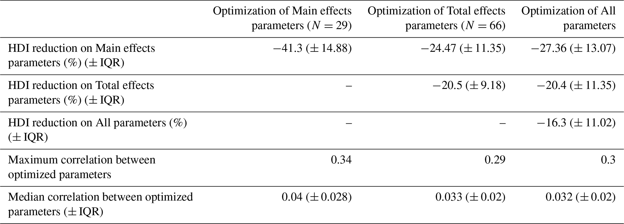
Table 5 Comparison of the number of 1D simulations and the computational cost required for the parameter screening and optimization steps. The screening step for identifying Main Effects and Total Effects parameters requires the same number of 1D simulations, and therefore the same computational cost. The same parameter optimization process is applied across all parameter sets. As a result, for the parameter optimization step the number of simulations and the associated computational cost are identical for each method. The computational cost is expressed in terms of CPU hours required to generate the full ensemble of 1D simulations on a single CPU of an HPC system. Naturally, this value depends on the number of nodes and the specific configuration of the HPC used. The computational cost of other steps, such as metric evaluation, is negligible compared to that of generating the 1D simulation ensemble.

4.7 Transferability of the optimized Parameters to the 3D Configuration

The 3D validation dataset comprises approximately 1430 unique BGC-Argo profiles matched to the IBI model over the period 2017–2019 (Fig. 10b). After quality control and outlier filtering, this yields between 430 000 and 490 000 observation–model pairs per variable across the 0–500 m depth range. The observation distribution is strongly asymmetric: the Mediterranean basin concentrates 85 %–90 % of the matched pairs, while the North Atlantic (Northern + Iberian Atlantic) contributes the remaining 10 %–15 %, reflecting the denser BGC-Argo float deployment in the Mediterranean during this period.

Table 6 Basin-level NRMSE for the OPTI and REF simulations and relative improvement Δ%NRMSE. Bold entries indicate NRMSE < 1 (performance within observation uncertainty). When both simulations are in bold, a positive Δ%NRMSE does not constitute a meaningful degradation.

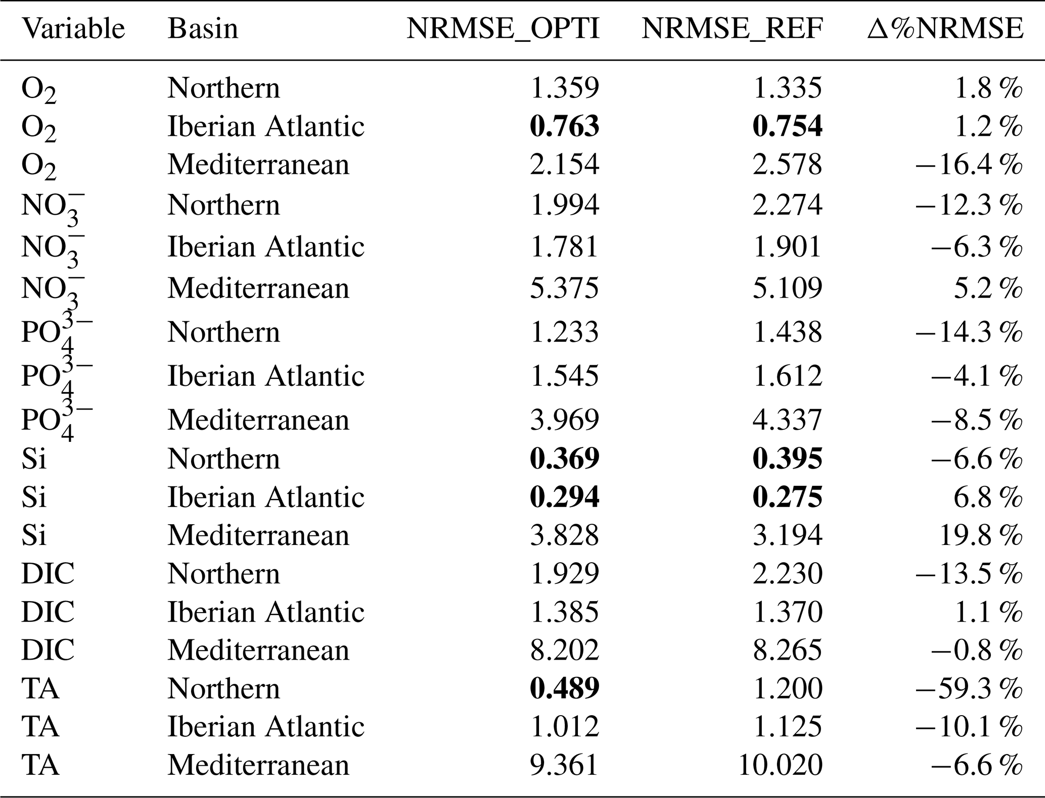
The OPTI simulation generally outperforms REF across the IBI domain (Table 6). Of the 18 variable–basin combinations, 12 show a negative Δ%NRMSE, indicating that the optimized parameters improve model skill. The largest improvements occur for total alkalinity in the Northern basin (Δ%NRMSE $=-\mathrm{59.3}$ %), dissolved oxygen in the Mediterranean (−16.4 %), phosphate in the Northern basin (−14.3 %), and DIC in the Northern basin (−13.5 %). Phosphate is the only variable for which OPTI outperforms REF in every basin, with Δ%NRMSE ranging from −4.1 % to −14.3 %.

Across basins, the Northern and Iberian Atlantic show the largest improvements. Nitrate, phosphate, and total alkalinity show consistent improvements in both basins, with Δ%NRMSE ranging from −4.1 % (PO${}_{\mathrm{4}}^{\mathrm{3}-}$, Iberian Atlantic) to −59.3 % (TA, Northern basin). DIC improves markedly in the Northern basin (−13.5 %) but remains essentially unchanged in the Iberian Atlantic (+1.1 %). These improvements are genuine because, for these variables, NRMSE values exceed unity in at least one simulation, confirming that the optimization measurably reduces model errors that are detectable relative to observation uncertainty. Dissolved oxygen is the only variable where OPTI slightly underperforms REF in the Northern basin (+1.8 %), though both simulations exceed unity only marginally. Silicate stands apart: both simulations achieve NRMSE well below unity (0.27–0.40) across both basins, indicating that the model reproduces CANYON-B-derived silicate observations within less than half the associated uncertainty regardless of the parameter set.

The Mediterranean presents a more contrasted picture. All NRMSE values exceed unity – by factors of 2 to 10 – indicating that model errors surpass observation uncertainty in this basin. Dissolved oxygen and phosphate show genuine improvements (Δ%NRMSE $=-$16.4 % and −8.5 %, respectively), confirming that the optimized parameters partially correct the free-running model even in a biogeochemical regime different from the training site. Nitrate and silicate, however, degrade under OPTI (+5.2 % and +19.8 %), suggesting that the biological rate parameters tuned on a single North Atlantic float do not fully transfer to the oligotrophic Mediterranean, consistent with the nitracline bias identified in the 1D independent validation (Sect. 4.6). The carbonate system variables exhibit very high NRMSE values (8–10 for both DIC and TA), reflecting the fact that the CONTENT-derived error estimates are much smaller than the actual model–observation discrepancies; within this context, OPTI provides only marginal improvements (−0.8 % and −6.6 %, respectively).

Surface chlorophyll a provides a complementary, independent assessment of the optimized parameters (Fig. 10). The Taylor diagram confirms that both simulations reproduce the MOBTAC-observed seasonal cycle across all five boxes with correlations typically exceeding 0.8–0.9. The OPTI simulation outperforms REF: for every box, the green markers sit closer to the MOBTAC reference point than the corresponding red markers, reflecting both a reduced centred RMSE and a normalised standard deviation brought closer to unity. The improvement is most visible in the Atlantic box 1 where REF tends to underestimate the amplitude of the seasonal cycle – a bias that the optimized parameters correct.

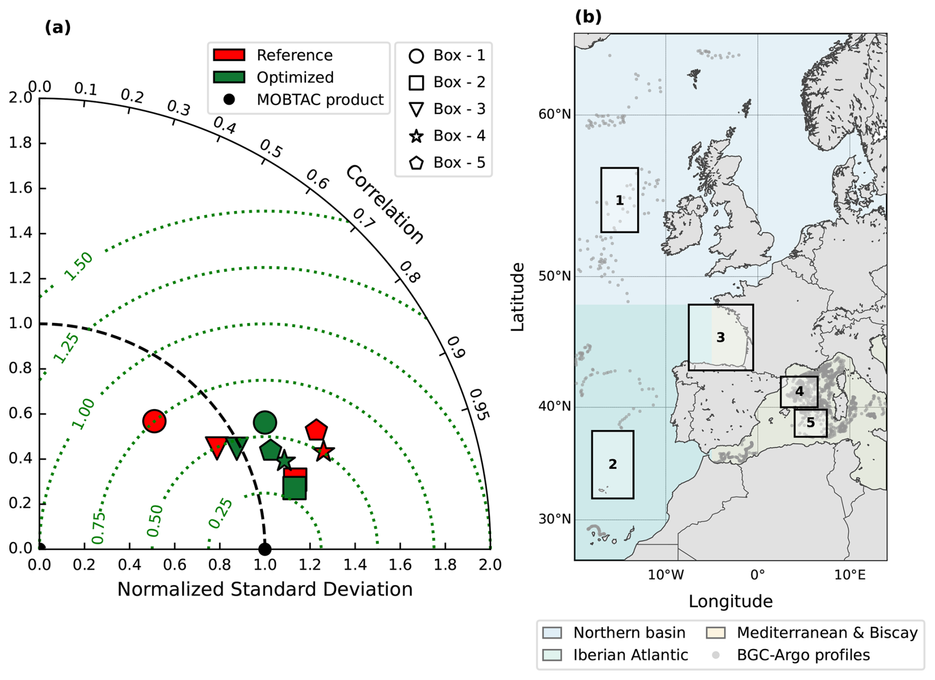
Figure 10 Surface chlorophyll a validation against the MOBTAC multi-observation reprocessed product over the period 2017–2019. (a) Taylor diagram computed on monthly mean time series in log₁₀ space. The radial distance from the origin represents the normalised standard deviation (${\mathit{\sigma }}_{\mathrm{model}}/{\mathit{\sigma }}_{\mathrm{obs}}$), the angular position the Pearson correlation coefficient, and the green dotted contours the centred root-mean-square difference. Red markers denote the REF simulation and green markers the OPTI simulation; marker shapes identify the five validation boxes (circle: Box 1; square: Box 2; inverted triangle: Box 3; star: Box 4; pentagon: Box 5). The black filled circle indicates the MOBTAC reference point at unit normalised standard deviation, and the black dashed semicircle marks the locus where model and observed variability are equal (${\mathit{\sigma }}_{\mathrm{model}}/{\mathit{\sigma }}_{\mathrm{obs}}=\mathrm{1}$). (b) Location of the five validation boxes within the IBI domain: Box 1 (Celtic Sea/Rockall Trough), Box 2 (Canary/Madeira), Box 3 (Bay of Biscay), Box 4 (Gulf of Lion), and Box 5 (Balearic Sea). The three broader sub-regions for subsurface BGC-Argo validation are delineated by colored polygons: Northern basin (20° W–17° E, 48–65° N), Iberian Atlantic (20–5° W, 26–48° N), and Mediterranean and Bay of Biscay (5° W–17° E, 26–48° N). Individual profile locations from the approximately 1430 BGC-Argo profiles matched to the IBI model over 2017–2019 are shown as grey dots.

5 Discussion

Our study demonstrates that assimilating a comprehensive suite of BGC-Argo observations from a single seasonal cycle improves the fit of the PISCES biogeochemical model in the productive layer by over 50 % (NRMSE), even with all 95 parameters perturbed simultaneously. Iterative Importance Sampling (iIS) reduced the productive-layer NRMSE by over 50 % relative to the reference simulation with default parameters and produced posterior distributions with negligible inter-parameter correlation (median r<0.04). The observations did not, however, constrain all 95 parameters equally: the median reduction in the 67 % HDI was 27 % for the most influential parameters but only 16 % across all 95, leaving most parameters weakly constrained. Directly optimizing all 95 model parameters yields the same goodness of fit as targeting smaller, GSA-informed subsets, with both approaches yielding statistically indistinguishable improvements in goodness of fit. Furthermore, all strategies produced ensembles with low bias and reliable, albeit cautious, uncertainty envelopes when evaluated against independent BGC-Argo observations. Given that the “All-parameters” strategy matches the other strategies' skill while avoiding the computational cost of the prerequisite GSA and providing a fuller accounting of parametric uncertainty propagated to unassimilated variables by retaining all parameters unfixed rather than arbitrarily constraining subsets. We therefore recommend this full-parameter optimization approach for high-dimensional Bayesian parameter estimation of biogeochemical models constrained by multi-variable observations (Table 5).

In complex biogeochemical models, parameter correlations, identifiability, and overfitting are closely linked. When two or more parameters produce compensating effects on the same model output, their posteriors become correlated, meaning they cannot be estimated independently from the available data – the parameters are said to be unidentifiable. Unidentifiable parameters are a direct pathway to overfitting: the optimization may find parameter combinations that reproduce the training data well, but for the wrong mechanistic reasons, leading to poor performance on independent observations. Breaking these correlations therefore requires observations that respond differently to each parameter, so that the data can distinguish their individual contributions. This is the rationale for assimilating a comprehensive, multi-variable dataset spanning multiple biogeochemical tracers.

A notable contribution of this framework is the transformation of parameter equifinality from a correlated state to an uncorrelated one, a longstanding challenge in biogeochemical data assimilation. Historically, studies using sparse datasets have often found strong posterior correlations between parameters, indicating that the available data were insufficient to constrain them independently (Matear, 1995; Hurtt and Armstrong, 1996; Fennel et al., 2001; Mamnun, 2022). Our results indicate that the comprehensive, multi-variable BGC-Argo dataset provides sufficient independent information to achieve uncorrelated equifinality: although multiple optimal parameter sets exist, the parameters within them vary independently rather than through compensating trade-offs. Simple trade-offs that cause parameter correlations in data-poor scenarios are no longer possible when twenty distinct metrics are assimilated simultaneously. These twenty metrics do not define separate objective functions optimized via multi-objective methods (Sauerland et al., 2019); rather, they enter a single product likelihood (Eq. S14), so that each ensemble member is evaluated against all constraints at once. For example, while increasing the P-I slope or decreasing phytoplankton mortality might both fit Chl a data, these changes leave different imprints on nitrate drawdown, oxygen concentrations, etc. As a result, the posterior parameter distributions show negligible inter-correlation (median r<0.04; Table 4). Rather than artificially fixing poorly constrained parameters at their default values, the framework allows all parameters to vary independently, providing ensemble-based uncertainty estimates that more faithfully represent the true confidence limits of the model.

A limitation of the present study concerns the range of conditions over which the optimized parameters remain valid. The independent-float and 3D validations already show that the parameters carry a real dependence on the environmental regime: the North-Atlantic-tuned set degrades nitrate and silicate in the contrasting oligotrophic Mediterranean. These validations do not, however, probe extrapolation beyond the present-day range – in particular to the warmer temperatures and altered nutrient supply expected under climate change. Such sensitivity is expected, because many of the optimized parameters enter temperature-dependent rate expressions and the optimization was constrained by a single site over one seasonal cycle. This bears directly on the climate-projection applications (e.g. CMIP6) that motivate this work: a parameter set tuned to present-day conditions may lose validity under future regimes, ultimately requiring periodic re-calibration or adaptive parameterizations that respond to the ambient state.

A recurrent concern in biogeochemical parameter optimization is whether parameters estimated in simplified 1D configurations compensate for missing physical processes rather than improving the biogeochemical formulation (Löptien and Dietze, 2019; Pasquier et al., 2023). The 3D validation directly addresses this question. Implementing the 1D- optimized parameter set from the All parameters strategy in the high-resolution IBI model – which resolves 3D physical processes – shows that skill improvements persist: the OPTI simulation outperforms REF in 12 of 18 variable–basin combinations, with the largest gains for total alkalinity, nitrate, and phosphate in the North Atlantic. Surface Chl a is also better reproduced across the entire domain. These results demonstrate that the 1D optimization has captured improvements in the biogeochemical parameterisation that transfer to a fully three-dimensional, dynamically resolved configuration.

The 3D validation does, however, reveal the regional specificity of the optimized parameter set. In the Mediterranean, OPTI degrades nitrate (+5.2 %) and silicate (+19.8 %) relative to REF, consistent with the nitracline bias already identified in the 1D independent validation against the Mediterranean float (Sect. 4.6). The North Atlantic-tuned biological rate parameters maintain a shallow nitracline structure that is inappropriate for the oligotrophic Mediterranean. This finding aligns with studies showing parameter variation across oceanic biomes (Singh et al., 2025) and motivates a move beyond a single global parameterization towards regionally-optimized parameter sets. Systematically applying this framework to the growing global fleet of BGC-Argo floats could enable the construction of parameter maps, revealing how PISCES parameters vary across the world's oceans and defining emergent “parameter bioregions”

The 1D vertical model used for the optimisation has both advantages and limitations. The primary advantage is computational efficiency: the 1D configuration reduces the cost of each ensemble member by several orders of magnitude relative to a 3D run, making it feasible to evaluate over 26 000 parameter combinations and to perform a rigorous global sensitivity analysis. The 1D model is forced offline with temperature, salinity, and vertical diffusivity from the CMEMS-PHY analysis. The CMEMS-PHY analysis reproduces the float-observed temperature and salinity reasonably well (Fig. 2), but the vertical mixing cannot be independently validated against BGC-Argo observations, as this variable is not measured by the floats. Because the parameters are tuned to reproduce the observations under this prescribed forcing, any bias in the CMEMS-PHY mixing could be partly absorbed into the calibrated parameters. In other words, part of the calibration may compensate for errors in the physical forcing rather than reflect true biological parameter values (Löptien and Dietze, 2019). We did not test how the optimized parameters would change under substantially different mixing conditions. Nevertheless, these parameters improve the 3D regional model, which uses its own dynamically simulated physics rather than the offline CMEMS-PHY physical forcing used in the 1D experiments. This suggests that the optimized parameters are not strongly tuned to the CMEMS-PHY mixing field, although the transferability remains only partial, as discussed in Sect. 4.7. The optimization is further conditioned on a single training site and a one-year assimilation window, which may not capture the full range of environmental variability encountered in multi-year, basin-scale applications. The 3D validation demonstrates that the optimized parameters improve model performance at locations far from the training site relative to the reference parameter set, which largely mitigates the single-site concern, although they may not be optimal for the IBI 3D simulation. Nevertheless, extending the assimilation window to multiple years and multiple sites would further strengthen confidence in the generality of the results.

6 Conclusions

We developed and applied a parameter optimisation framework that leveraged comprehensive BGC-Argo data from a North Atlantic float in order to constrain the 95 parameters of the PISCES biogeochemical model. This framework reduced the productive-layer model-data misfit by over 50 % and yielding decorrelated posterior parameter distributions. These advance shifts the long-standing challenge of correlated equifinality to uncorrelated equifinality, where a range of optimal parameter sets can be found independently.

Directly optimizing all 95 parameters without a prerequisite GSA is the recommended strategy. Optimising the full parameter set achieves statistically indistinguishable skill improvements compared to targeting smaller, GSA-informed subsets, without incurring the immense computational cost of a prerequisite GSA. By exploring the full 95-parameter space, direct optimisation provides a fuller accounting of parametric uncertainty for unassimilated variables than optimising smaller, GSA-informed subsets.

The optimized parameters improve not only the 1D simulations on which they were trained, but also the three-dimensional, high-resolution IBI simulation against independent observations, at least, off the continental shelf. The 3D validation against approximately 1430 BGC-Argo vertical profiles and the MOBTAC surface Chl a product confirms that OPTI outperforms REF in the majority of variable–basin combinations. However, some regional specificity remains: in the Mediterranean, nitrate and silicate show degraded skill. This demonstrates that a 1D optimisation trained on a single North Atlantic BGC-Argo float can yield parameter sets that improve an operational 3D biogeochemical model simulation in the IBI domain.

Two avenues remain to be explored. The generality of the single-float 1D Bayesian optimisation framework should be tested by applying it to additional BGC-Argo floats in other oceanic regions, and the resulting parameter sets should be evaluated to determine whether they further improve model performance across biogeochemically distinct basins. Whether the optimized parameters stay stable and transferable across other observational datasets – different temporal windows or subsets from the same float, and floats from other biogeochemical regions – was not assessed here and remains to be tested. A further priority is to enrich the observation vector with zooplankton constraints, given that our GSA identifies zooplankton-related parameters as the dominant source of model sensitivity. The recent development of the Underwater Vision Profiler 6 (UVP6; Picheral et al., 2022), a miniaturised imaging sensor that can be integrated on BGC-Argo floats, may in the future provide zooplankton abundance profiles from the same autonomous platforms, offering a direct pathway to constrain the grazing parameters.