CO₂ and H₂O isotope exchange and flux partitioning in Amazonia

Understanding the coupled exchange of H₂O and CO₂ between ecosystems and the atmosphere remains limited due to our inability to partition net fluxes into their individual source and sink components. For the Amazon rainforest, which plays an important role in the global balance of water and carbon, investigating these individual fluxes is critical given the environmental changes in recent years. Here, we apply a stable isotope-based approach to partition ecosystem-scale gas exchange from simultaneous eddy covariance measurements of H₂O and CO₂ isotopologues. During the 2022 CloudRoots-Amazon campaign at the Amazon Tall Tower Observatory, high-frequency isotopologue flux measurements from 57 m were used to derive multi-day composite diurnal cycles of δ fluxes and ecosystem source compositions. A steady-state midday interval, constrained with independent leaf and soil isotopic observations, allowed us to coherently link the H₂O and CO₂ isotopic states throughout the ecosystem (soil, canopy, leaf, atmosphere) using δ¹⁸O.

Isotopic flux partitioning indicates that transpiration accounts for 95.5 % of the net evapotranspiration (ET) of water at 14:00 LT (all times are local time), with soil evaporation being responsible for 4.5 %. For CO₂, δ¹⁸O-based partitioning indicates that the respiration flux from the soil equals −44 % of the net ecosystem exchange (NEE), where the photosynthetic assimilation flux in turn is 144 % of NEE. The partitioning of NEE was found to be strongly dependent on the leaf intercellular-to-atmospheric CO₂ ratio ($c_{\mathrm{i}}/c_{\mathrm{a}}$) which determines the (apparent) isotopic composition associated with photosynthetic assimilation (δ_P). This underlines how important detailed leaf and soil level measurements of isotopic compositions and leaf characteristics are for ecosystem-scale flux partitioning.

1 Introduction

Tropical rainforests are key drivers of the global water and carbon cycles (Bastos et al., 2020; Dominguez et al., 2022). However, the dynamics of these ecosystems are changing as a result of deforestation and climate change (Artaxo, 2023; Espinoza et al., 2024). The Amazon rainforest, which is world's largest, is changing from a net carbon sink to a source (Brienen et al., 2015; Ke et al., 2024). Unprecedented droughts and forest fires in recent years are signals of that change (Moreira et al., 2024; Mataveli et al., 2024).

Ecosystem scale measurements of the gas exchange of H₂O and CO₂ enable us to understand ecosystem dynamics (Baldocchi, 2014). However, common approaches for measuring the exchange are only able to assess the net exchange, which is the sum of several individual processes. The net ecosystem exchange of carbon dioxide (NEE) is the sum of the uptake by photosynthesis (P) and the release by respiration (R). Here, R is the sum of photo-respiration, dark respiration, and heterotrophic respiration. For water vapour, the main components of the net Evapotranspiration (ET) flux are the transpiration from vegetation (T), and evaporation (E) from soils. Note that after precipitation or during dewfall, a separate evaporation flux from intercepted water might be defined (Wei et al., 2017).

The inability to measure individual ecosystem fluxes separately is an important limitation in advancing our understanding of ecosystem dynamics. This is because environmental drivers are linked to individual gross fluxes, and relate only indirectly to net fluxes (Tramontana et al., 2020; Stoy et al., 2019). These process-based individual fluxes can be implemented in mathematical models to understand the relative importance and possible changes in individual exchange processes. Soil and leaf scale measurements provide accurate individual fluxes at small scales, but connecting those to the canopy and ecosystem scale is challenging (Sabot et al., 2022; González-Armas et al., 2024; Mangan et al., 2023). Stable isotopes can serve as natural tracers to address this limitation.

The isotopic composition is generally expressed in δ-notation, which is defined as:

$$\begin{array}{}\text{(1)}& \mathit{\delta }={\displaystyle \frac{R_{\mathrm{spl}}}{R_{\mathrm{ref}}}}-\mathrm{1}\end{array}$$

where R_spl indicates the heavy-to-light isotope ratio of the sampled compound, and R_ref represents the same isotope ratio of a common reference material (Mook and Geyh, 2000). In this work, we focus on the D isotope in H₂O, and the ¹⁸O isotope in both H₂O and CO₂, for which Vienna Standard Mean Ocean Water (VSMOW) is the common reference (^DR_ref= 0.00015575 and ¹⁸R_ref= 0.0020052).

In natural ecosystems, small differences (‰) occur between the rate of exchange of various isotopologues dependent on the process. These differences can be used to attribute changes in isotopic compositions to specific environmental exchange processes, such as transpiration. For the application of ecosystem flux partitioning, flux measurements of the isotopic composition in the atmosphere δ_atm must be made in combination with measurements of the isotopic compositions of the relevant exchange reservoirs, e.g., soil water, leaf water or soil carbon isotopic composition (Barbour et al., 2017; Wehr and Saleska, 2015). In Sect. 2 we define the δ fluxes and describe how the ecosystem end-member compositions are quantified making use of collocated measurements of environmental variables and isotopic compositions.

Isotopic flux partitioning can be applied to all relevant isotopologues, potentially offering multiple, complementary handles. For example, water fluxes can be constrained independently using both ¹⁸O and D isotopes. ¹⁸O provides an interesting cross-species link because ¹⁸O exchanges rapidly between H₂O and CO₂ in leaves, catalysed by the enzyme Carbonic Anhydrase (CA). For this reason, ¹⁸O has shown to be a valuable link between the carbon and water cycles (Gillon and Yakir, 2001).

In this work, we aim to use the ¹⁸O isotopic signature in both H₂O and CO₂ to describe the isotopic state throughout the ecosystem in detail, which should allow for the net fluxes of H₂O and CO₂ to be partitioned into seperate soil and vegetation fluxes. To this end, we make use of comprehensive measurements of H₂O and CO₂ isotopic fluxes, vertical profiles of the state variables and discrete air, leaf and soil water isotopic samples, and leaf gas exchange measurements. We base our analysis on the CloudRoots-Amazon22 dataset, which was acquired at the Amazon Tall Tower Observatory (ATTO) site in Brazil (see Sect. 3). We describe the diurnal cycles of the observed isotopic fluxes and discuss the isotopic state of the ecosystem. For a midday steady state period we then determine the end member isotopic compositions of individual gross fluxes. This allows us to systematically partition the net ecosystem fluxes into its individual components, which enables high resolution simulations of the water and the carbon cycles to be validated (Pedruzo-Bagazgoitia et al., 2023). In addition, our observations help to probe our biogeochemical understanding of the ¹⁸O exchange at the ecosystem scale (Farquhar and Lloyd, 1993).

2 Theory

Stable isotope measurements of atmospheric species can be used to partition multiple sources and sinks of the same compound, which cannot be done with mole fraction information only (Wehr and Saleska, 2015; Oikawa et al., 2017). Mathematically, a system of two exchange equations is solved for two source fluxes. Given the land-atmosphere exchange of H₂O, it can be applied to partition evapotranspiration (ET) into evaporation (E) and transpiration (T). In this section, we first detail ET partitioning using the stable deuterium (D) isotope and subsequently show how the NEE of CO₂ can be partitioned into P and R using the ¹⁸O isotope. Note that in the results, both the D and ¹⁸O signatures of H₂O are used for ET partitioning. The following set of equations is specific to the example of ET partitioning using D, but can be used for NEE and ¹⁸O as well (Bowling et al., 2001).

$$\begin{array}{}\text{(2)}& \begin{array}{rl}\mathrm{ET}& =E+T\\ \mathit{\delta }{\mathrm{D}}_{\mathrm{ET}}\cdot \mathrm{ET}& =\mathit{\delta }{\mathrm{D}}_{\mathrm{E}}\cdot E+\mathit{\delta }{\mathrm{D}}_{\mathrm{T}}\cdot T\end{array}\end{array}$$

Here, δD_ET is the deuterium isotopic composition of the net water vapour flux due to both evaporation and transpiration, δD_E is the isotopic composition of the evaporated water, and δD_T of the transpired water. This approach enables us to constrain a system with two individual gross fluxes contributing to the net flux. When more source terms are described, other isotopic or non-isotopic constraints can be added, or a-priori assumptions between the tracers need to be used. For the system represented in the above equations, none of the three isotope parameters (δD_ET, δD_E, and δD_T) are easily obtained and in the following section we describe the methods to acquire each of them.

2.1 The isotopic composition of the net exchange flux

The isotopic composition of the net exchange flux (δ_ET or δ_NEE) is comparable to the source isotopic composition being mixed into a reservoir. The difference is that δ_ET and δ_NEE can also describe the composition of a negative (uptake) flux. The common approach for determining the isotopic composition of a source from atmospheric measurements are mixing models, as described by Keeling (1958) and Miller and Tans (2003). In these models, changes in atmospheric isotopic compositions are directly related to changes in mole fractions. For example, when increased mole fractions are associated with enriched isotopic compositions, the source is understood to be more enriched than the atmospheric background. In the Miller-Tans (MT) method, the slope of the relationship between δχ and χ is solved for to find the isotopic composition of the source (example in Appendix Fig. A1). In various studies, the MT method has been used to determine δ_ET or δ_NEE irrespective of the flux sign (Griffis, 2013; Finkenbiner et al., 2022). We refer to estimates using the MT methods with δ_…,MT.

The isotopic composition of the net turbulent exchange flux can also be estimated with measurements of the turbulent exchange fluxes of the various isotopologues of the target species (Griffis et al., 2007). δ fluxes (F_δ) provide a common method to determine such an isotopologue flux.

$$\begin{array}{}\text{(3)}& F_{\mathit{\delta }}=\stackrel{\mathrm{‾}}{w^{\prime }{\mathit{\delta }}^{\prime }}\end{array}$$

where, w^′ and δ^′ are the fluctuating components of the vertical wind and isotopic composition, respectively, after Reynolds decomposition (Bird, 2002). F_δ has the units ‰ m s⁻¹. For the example of δD in water, F_δD is related to the isotopic composition of the net flux (δD_ET), the atmospheric isotopic composition (δD_atm), and the total exchange flux (in this case ET) as follows (Lee et al., 2012).

$$\begin{array}{}\text{(4)}& F_{\mathit{\delta }\mathrm{D}}={\displaystyle \frac{\mathrm{ET}}{{\mathit{\rho }}_v^{\mathrm{atm}}}}\cdot (\mathit{\delta }{\mathrm{D}}_{\mathrm{ET},\mathrm{F}}-\mathit{\delta }{\mathrm{D}}_{\mathrm{atm}})\end{array}$$

Here, ET is the evapotranspiration flux in $\mathrm{g}{\mathrm{m}}^{-\mathrm{2}}{\mathrm{s}}^{-\mathrm{1}}$. ${\mathit{\rho }}_v^{\mathrm{atm}}$ is the atmospheric absolute humidity in g m⁻³, and δD_atm is the atmospheric isotopic composition of deuterium in water vapour. Note that the fraction $\frac{\mathrm{ET}}{{\mathit{\rho }}_v^{\mathrm{atm}}}$ defines an exchange rate. The unit grams in the nominator and denominator can thus be replaced by moles. The isotopic composition of the net exchange flux (δD_ET), determined using this flux method (δ_…,F), can be solved for and inserted into Eq. (2).

Until recently, the δ flux (F_δ) could only be inferred by relating gradient measurements of isotopologues to an exchange coefficient depending on mechanical and convective turbulence (Griffis et al., 2004; Yakir and da Silveira Lobo Sternberg, 2000). At present, high flow rate laser spectrometers are available which measure the isotopic composition at sub-second frequencies, which allow for direct isotopologue flux measurements using the eddy covariance technique (Griffis, 2013; Sturm et al., 2012; Wahl et al., 2021). The difficultly in using such measurements is keeping the instrument stable, while maintaining high flow rates and an undisturbed inlet gas stream, which is necessary to resolve both the longest and shortest turbulent exchange timescales (Kolmogorov, 1941). We found that temperature-stabilized enclosures, combined with short, heated inlet lines provide a workable mode of adhering to these constraints (see Sect. 3).

2.2 The H₂O isotopic state

2.2.1 The isotopic composition of soil evaporation

Soil water samples can inform us of the isotopic composition of the soil evaporation δD_E, which is required to solve Eq. (2). When calculating the isotopic composition of water evaporating from soils from the soil water isotopic composition, the temperature dependent isotopic fractionation of the liquid-to-gas phase change (evaporative fractionation) needs to be taken into account. The isotopic fractionation factor for deuterium (α_{l-v, D}) as determined by Horita and Wesolowski (1994) is:

$$\begin{array}{}\text{(5)}& \begin{array}{rl}{\mathrm{10}}^{\mathrm{3}}\ln & \left({\mathit{\alpha }}_{\text{l-v, D}}\right)=\mathrm{1158.8}(T^{\mathrm{3}}/{\mathrm{10}}^{\mathrm{9}})-\mathrm{1620.1}(T^{\mathrm{2}}/{\mathrm{10}}^{\mathrm{6}})\\ & +\mathrm{794.84}(T/{\mathrm{10}}^{\mathrm{3}})-\mathrm{161.04}+\mathrm{2.9992}({\mathrm{10}}^{\mathrm{9}}/T^{\mathrm{3}})\end{array}\end{array}$$

Here, T is the temperature expressed in K, α_{l-v, D} is the isotopic fractionation factor for deuterium when transitioning from a liquid (l) to a vapour (v) state.

For a given deuterium isotopic composition of liquid soil water, the isotopic fractionation factor can be used to calculate the equilibrium isotopic composition of the water vapour with (Mook and Geyh, 2000):

$$\begin{array}{}\text{(6)}& R_{\mathrm{D},\mathrm{v}}=R_{\mathrm{D},\mathrm{ref}}({\mathit{\delta }}_{\mathrm{D},\mathrm{v}}+\mathrm{1})={\displaystyle \frac{R_{\mathrm{D},\mathrm{l}}}{{\mathit{\alpha }}_{\text{l-v, D}}}}\end{array}$$

See Eq. (1) to see how the isotope ratios (R in Eq. 6) relate to δ values. The main simplification in using the equilibrium water vapour isotopic composition to estimate δ_E is that kinetic fractionation effects taking place during diffusion into the atmosphere are not taken into account. Physically accurate representations of this kinetic fractionation are available, but complex. Kiemle et al. (2023) share a full complexity model, and find that using equilibrium fractionation only is a good first order approximation.

2.2.2 The isotopic composition of transpiration

Generally, the isotopic composition of δD_T is set equal to the isotopic composition of the source water in the soil (δD_S), using the assumption of isotopic steady-state (Craig and Gordon, 1965). This is an expansion of the idea that when taking the leaf as a reservoir, the mass of the water entering the leaf matches the mass of the water evaporating from the leaf. Analogous to mass, no isotopologue species should be able to accumulate in leaves on longer timescales (Farquhar and Cernusak, 2005; Barbour et al., 2017). On short timescales, the leaf water will act as a buffer when environmental conditions are changing (Dongmann et al., 1974).

The (δD_S) taken up by a plant represents the average of the water isotopic gradient in the root zone, weighted by the root water uptake at each depth (De Deurwaerder et al., 2020; Sutanto et al., 2014). This composition can be determined directly from a tree by sampling the water in the xylem. There is no fractionation associated with root water uptake, or transport through a tree (Rothfuss and Javaux, 2017).

2.2.3 The isotopic composition of water at evaporation sites

The average liquid water isotopic composition of leaves can be determined by collecting and analysing leaf samples. However, the isotopic composition of transpiration is related specifically to the water isotopic composition at the evaporation site in the stomata. The Craig-Gordon model, following Farquhar et al. (2007), accounts for the bidirectional isotopic exchange between atmospheric water vapour and the liquid water at the evaporation site.

$$\begin{array}{}\text{(7)}& R_{\mathrm{e}}={\mathit{\alpha }}_{\text{l-v}}\left[{\mathit{\alpha }}_k{R}_{\mathrm{s}}\left(\mathrm{1}-{\displaystyle \frac{w_{\mathrm{a}}}{w_{\mathrm{i}}}}\right)+R_{\mathrm{v}}{\displaystyle \frac{w_{\mathrm{a}}}{w_{\mathrm{i}}}}\right]\end{array}$$

Here, R_e is the isotope ratio of liquid water at the evaporation site, R_s is the isotope ratio of the liquid source water, R_v is the isotope ratio of atmospheric water vapour, and $\frac{w_{\mathrm{i}}}{w_{\mathrm{a}}}$ are the water vapour mole factions in the intercellular air space and in the atmosphere respectively.

The $w_{\mathrm{a}}/w_{\mathrm{i}}$ ratio can be interpreted as a relative humidity gradient and is used to describe the bidirectional diffusion of water vapour through stomata. Two terms in Eq. (7) contain the $w_{\mathrm{a}}/w_{\mathrm{i}}$ ratio, and together sum to 1. The $\mathrm{1}-w_{\mathrm{a}}/w_{\mathrm{i}}$ term is associated to newly evaporated water, while the $w_{\mathrm{a}}/w_{\mathrm{i}}$ term is instead related to back-diffusion of ambient vapour. Together, both determine R_e, with $w_{\mathrm{a}}/w_{\mathrm{i}}$ indicating which process has a proportionally larger influence. At a certain leaf temperature, the internal concentration w_i is generally assumed to be equal to the temperature dependent saturation vapour pressure. While we make use of this assumption, we are aware that Cernusak et al. (2024) recently reported that this assumption is not always valid. The $w_{\mathrm{a}}/w_{\mathrm{i}}$ ratio is referred to with the symbol h in some literature (Farquhar and Cernusak, 2005).

α^k is the kinetic fractionation describing the faster diffusion for the light, abundant isotopologues. Farquhar et al. (1989a) quantified this fractionation step using the widely-applied resistance formulation, as shown in Eq. (8).

$$\begin{array}{}\text{(8)}& {\mathit{\alpha }}_k\left(D\right)=\mathrm{1}+{\displaystyle \frac{\mathrm{0.025}{r}_{\mathrm{s}}+\mathrm{0.017}{r}_{\mathrm{b}}}{r_{\mathrm{s}}+r_{\mathrm{b}}+r_{\mathrm{a}}}}\end{array}$$

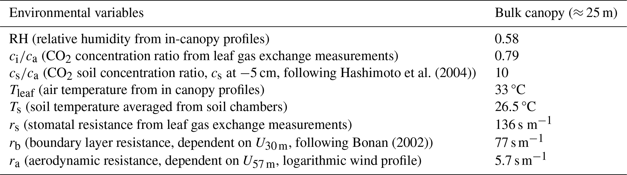
Here, r_s, r_b, and r_a are the stomatal, leaf boundary layer, and aerodynamic resistances respectively, in s m⁻¹. The numbers 0.025 and 0.017 originate from 1.025 and 1.017, which are the kinetic fractionation factors for HDO compared to HHO for stomatal and boundary layer diffusion, respectively (Farquhar et al., 1989a). For ¹⁸O, the kinetic fractionation factors are 1.032 for stomatal diffusion and 1.021 for the boundary layer diffusion (Lee et al., 2009). As transport to the atmosphere outside the leaf boundary layer is not a diffusive process, r_a does not cause kinetic fractionation. The used values for the resistances are specified in Table 1.

Hashimoto et al. (2004)Bonan (2002)

Table 1 Multi-day averaged 14:00 environmental and biospheric conditions during the CloudRoots-Amazon22 campaign at the ATTO site. The in-canopy scalar data and leaf gas exchange measurements were presented and interpreted in González-Armas et al. (2025).

The structure of Eq. (8) is the result of the transport pathway, where resistances associated to different physical transport processes (diffusion through stomata, diffusion though air in the leaf boundary layer, turbulent transport) are presented in series. Here, the largest resistance is the rate limiting step, and dominates the net fractionation effect. When the process is more diffusive, the related fractionation effect is larger. The theoretical kinetic fractionation factor for diffusion of HDO and HHO in free air, determined using the respective diffusivities (κ), is 1.0274. For diffusion through stomata or though the boundary layer this potential fractionation effect is reduced, as both processes are not purely diffusive. Boundary layer resistance is partially related to turbulent transport, which does not itself cause any fractionation (Lee et al., 2009). In contrast, transport through the stomata is near purely diffusive, resulting in larger fractionations factors, closer to the theoretical value. So far, empirical experiments have been used to quantify the fractionation factor specific to a context (Cappa et al., 2003).

2.2.4 The Péclet effect: Linking leaf samples to the evaporation site isotopic composition

A strong isotopic gradient can be present from the leaf veins to the evaporation site as a consequence of transpiration itself. This is because the light isotopologues evaporate preferentially from the liquid phase (Eq. 5), resulting in an enriched liquid water reservoir in the mesophyll. Back diffusion will act to diminish this gradient, but is limited during daytime due to the continual water flux from vein to the atmosphere, through the mesophyll (Cernusak et al., 2016).

The bidirectional scalar transport by advection and by diffusion results in a Péclet effect (Bird, 2002). Here, the dimensionless Péclet number (ϕ) indicates the relative magnitude of the advective flow compared to the diffusive relaxation, where numbers larger than one indicate advective dominance. In leaves, Péclet numbers are generally high during daytime, and low during nighttime, dependent on the transpiration flux T (Cernusak et al., 2016).

$$\begin{array}{}\text{(9)}& \mathit{\varphi }={\displaystyle \frac{TL}{{\mathit{\rho }}_{\mathrm{lw}}\mathit{\kappa }}}\end{array}$$

Here, T is the transpiration rate in $\mathrm{g}{\mathrm{m}}^{-\mathrm{2}}{\mathrm{s}}^{-\mathrm{1}}$, L is the length scale over which the Péclet effect takes place, which is approximated as k⋅l (Barbour et al., 2017), in which l is the distance between the veins and the stomata in m, and k is a dimensionless scaling factor which corrects for the tortuous path, ρ_lw is the density of liquid water g m⁻³, and κ is the diffusivity of the heavy isotopologue in m² s⁻¹ (Farquhar and Lloyd, 1993). Barbour and Farquhar (2004) determined that L=8 mm provides a reasonable length scale, with l estimated at 0.1 mm. For the Amazonian dry seaon specifically, Lai et al. (2008) reported a much higher average value of L=54 mm.

Taking the Péclet effect into account allows the water isotopic compositions of entire leaves to be linked to the isotopic composition at the evaporation site as follows.

$$\begin{array}{}\text{(10)}& {\mathit{\delta }}_{\mathrm{leaf}}={\displaystyle \frac{(\mathrm{1}-e^{\mathit{\varphi }})({\mathit{\delta }}_{\mathrm{e}}-{\mathit{\delta }}_{\mathrm{xylem}})}{\mathit{\varphi }}}+{\mathit{\delta }}_{\mathrm{xylem}}\end{array}$$

In reality, a series of Péclet effects, with multiple unique Péclet numbers takes place in the apoplastic cell tissue, minor veins, and major veins (Cernusak et al., 2016; Farquhar and Gan, 2003). Given that more complete formulations lack validation on key coefficients, Eq. (10) is generally used (Barbour et al., 2017). With the comprehensive data we collected, we were able to estimate a realistic value for L, which we describe in Sect. 4.3.

2.3 The CO₂ isotopic state

In this work, we focus on the δ¹⁸O isotopic state or isotopic cascade of CO₂ in the relevant reservoirs of the ecosystem, and on the isotopic link between CO₂ and H₂O. Our measurements also include δ¹³C and we show the time series of δ¹³C fluxes in Sect. 4.2, but do not investigate δ¹³C in the individual reservoirs. The reason for this is that δ¹³C has been thoroughly investigated to constrain the exchange of CO₂ on various scales (van der Velde et al., 2014; Wehr and Saleska, 2015; Oikawa et al., 2017). On global scales it has proven to be a highly valuable tracer for separating oceanic, fossil, and biospheric sources and sinks (Graven et al., 2020). At ecosystem scales however, the small isotopic disequilibrium between photosynthesis (P) and respiration (R) has been limiting for acquiring reliable partitioning results (Bowling et al., 2001; Griffis, 2013). The combined water and CO₂ isotopologue flux measurements performed during CloudRoots-Amazon22 provide a unique opportunity to explore the ecosystem flux partitioning using the δ¹⁸O-CO₂ cycle instead.

2.3.1 The δ¹⁸O-CO₂ isotopic composition associated with assimilation

The δ¹⁸O signature of CO₂ is largely determined by the isotopic composition of H₂O_l in the biosphere. Generally, the isotopic exchange between H₂O_l and CO_2,aq is relatively inefficient, as it is dependent on the slow hydration of CO₂ (CO₂ + H₂O ⇄ HCO${}_{\mathrm{3}}^{-}$ + H⁺). However, the enzyme Carbonic Anhydrase (CA), readily present in plants, accelerates this exchange by 6 orders of magnitude, which allows for sub-second isotopic equilibration (Nocentini et al., 2021). The isotope exchange between liquid H₂O and CO₂ taking place as a result of hydration, is associated with a fractionation effect. Brenninkmeijer et al. (1983) determined the magnitude of this temperature dependent effect to be

$$\begin{array}{}\text{(11)}& {\mathit{\alpha }}_{{\mathrm{H}}_{\mathrm{2}}\mathrm{O}\to {\mathrm{CO}}_{\mathrm{2}}}^{\mathrm{18}}=\mathrm{1}+{\displaystyle \frac{\mathrm{17.604}}{T_{\mathrm{K}}}}-\mathrm{17.93}\times {\mathrm{10}}^{-\mathrm{3}}\end{array}$$

where T_K is the temperature in K. In vegetation, CO₂ interacts with liquid water at the liquid-gas interface in the mesophyll, where evaporation takes place. The H₂O_l isotopic composition at the exchange site (δ_e) is determined using Eq. (7). The isotopic signature of CO₂ at these exchange sites (${\mathit{\delta }}_{\mathrm{c}}^{\mathrm{18}}$) can then be calculated by using Eq. (6), and applying ${\mathit{\alpha }}_{{\mathrm{H}}_{\mathrm{2}}\mathrm{O}\to {\mathrm{CO}}_{\mathrm{2}}}^{\mathrm{18}}$. Note that the abundance of water molecules is much larger than the abundance of CO₂ molecules which causes δ_e to be seemingly unaffected by the isotopic equilibration between H₂O_l and CO_2,aq.

To calculate the isotopic composition associated with assimilation in the canopy (δ_P), the bidirectional diffusion of CO₂ must be taken into account, in addition to the combined kinetic fractionation effects associated with transport across the stomata, the leaf boundary layer, and the atmospheric surface layer (Farquhar et al., 1993). We follow Lee et al. (2009) to solve for δ_P.

$$\begin{array}{}\text{(12)}& {\mathit{\delta }}_{\mathrm{P}}={\displaystyle \frac{{\mathit{\delta }}_{\mathrm{c}}^{\mathrm{18}}{c}_{\mathrm{i}}}{c_{\mathrm{i}}-c_{\mathrm{a}}}}+{\displaystyle \frac{{\mathit{\delta }}_{\mathrm{atm}}^{\mathrm{18}}{c}_{\mathrm{a}}}{c_{\mathrm{a}}-c_{\mathrm{i}}}}-{\mathit{ϵ}}_k\end{array}$$

Here, c_i and c_a are the CO₂ mole fraction in the intercellular air space and the atmosphere respectively µmol mol⁻¹. During day time, photosynthetic assimilation reduces c_i compared to c_a (Farquhar et al., 1989a; González-Armas et al., 2025). Even though the net transport of CO₂ is from the atmosphere to the leaf, back diffusion through the stomata brings equilibrated CO₂ into the atmosphere. This results in an apparent fractionation that appears to take place during δ¹⁸O-CO₂ uptake. However, the root cause of this signal is not fractionation during uptake, but isotopic equilibration between CO₂ and H₂O followed by back-diffusion of the equilibrated CO₂ to the atmosphere.

Gillon and Yakir (2001) found that not all CO₂ molecules that undergo back-diffusion had equilibrated with the leaf water, and estimated that the extent of CO₂ hydration in leaves (θ_eq) of forest ecosystems was 0.96. Incorporating this effect convolutes Eq. (12) to the following (Lee et al., 2009).

$$\begin{array}{}\text{(13)}& \begin{array}{rl}{\mathit{\delta }}_{\mathrm{P}}& ={\mathit{\theta }}_{\mathrm{eq}}\left({\mathit{\delta }}_{\mathrm{c}}^{\mathrm{18}}-{\mathit{\delta }}_{\mathrm{atm}}^{\mathrm{18}}\right){\displaystyle \frac{c_{\mathrm{i}}}{c_{\mathrm{i}}-c_{\mathrm{a}}}}-(\mathrm{1}-{\mathit{\theta }}_{\mathrm{eq}}){\mathit{ϵ}}_k{\displaystyle \frac{c_{\mathrm{i}}}{c_{\mathrm{a}}}}\\ & +{\mathit{\delta }}_{\mathrm{atm}}^{\mathrm{18}}-{\mathit{ϵ}}_k\end{array}\end{array}$$

2.3.2 The δ¹⁸O-CO₂ isotopic composition associated with soil respiration

In the soil, the hydration of CO₂ is also the main driver affecting δ¹⁸O-CO₂. The availability of carbonic anhydrase (CA) in soil water is generally lower compared to the availability in mesophyll water, and related to the number and types of soil microbes (Jones et al., 2021). Wingate et al. (2009) find that complete equilibration is generally achieved in the top 5 cm. The isotopic composition of soil water samples at 5 cm depth is thus used to calculate δ¹⁸O-CO_2 soil according to Eq. (11).

To derive the isotopic composition of soil respiration (δ_R), the bidirectional diffusion and fractionation associated with diffusion should be taken into account, as is done for the canopy in Eq. (13). Given the high concentrations of CO₂ in the soil, the effect of diffusion from the soil to the atmosphere is the dominant factor (Hashimoto et al., 2004). The formulation below takes into account the back-diffusion of air from the atmosphere into the soil (known as soil invasion; Tans (1998)).

$$\begin{array}{}\text{(14)}& {\mathit{\delta }}_{\mathrm{R}}={\displaystyle \frac{{\mathit{\delta }}_{\mathrm{soil}}^{\mathrm{18}}{C}_{\mathrm{s}}}{C_{\mathrm{s}}-C_{\mathrm{a}}}}+{\displaystyle \frac{{\mathit{\delta }}_{\mathrm{atm}}^{\mathrm{18}}{c}_{\mathrm{a}}}{c_{\mathrm{a}}-C_{\mathrm{s}}}}-{\mathit{ϵ}}_{\mathrm{k},\mathrm{s}}\end{array}$$

Here, C_s is the CO₂ mole fraction of the air in the soil µmol mol⁻¹.

3 Data collection and treatment

This study integrates data collected during the 2-week CloudRoots-Amazon22 campaign, which took place at the ATTO (Amazon Tall Tower Observatory) site in Brazil (González-Armas et al., 2025; Vilà-Guerau de Arellano et al., 2024; Moonen et al., 2025a). The campaign took place during the dry season and it was characterized by days with clear skies in the morning, which developed into shallow cumulus cloud fields later in the day (de Feiter et al., 2025). Central to the isotopic δ flux measurements and associated ecosystem source compositions was an Eddy Covariance (EC) setup installed at 57 m (see Fig. 1). This height was ≈ 25 m above the canopy, and is representative for the ecosystem scale (10⁵ m² footprint). The EC system consisted of a CSAT3 anemometer (Campbell Scientific, Logan, USA) and a LI-COR 7500 open path gas analyser (OPGA, LI-COR Inc, Lincoln, U.S.A.). Two laser spectrometers with high flow rates were placed on a tower balcony at 54 m height with an 8 m inlet to the anemometer (Fig. 1). This inlet line was a $\mathrm{1}/{\mathrm{2}}^{\prime \prime }$ (12.7e−3 m) copper tube which was heated and insulated, and protected from the environment with an aluminium mesh inlet filter. The flow rate exceeded 20 L min⁻¹ to provide turbulent conditions which preserved high-frequency fluctuations in the air stream (Moonen et al., 2023). The CO₂ isotope analyser used was an Aerodyne TILDAS-CS laser spectrometer (Aerodyne Research Inc., Billerica, USA) and the water isotope analyser was a Picarro L-2130i (Picarro, Santa Clara, USA). Both were placed in temperature controlled enclosures set to 35 °C. These stabilised the temperature sensitive instruments, while preventing condensation.

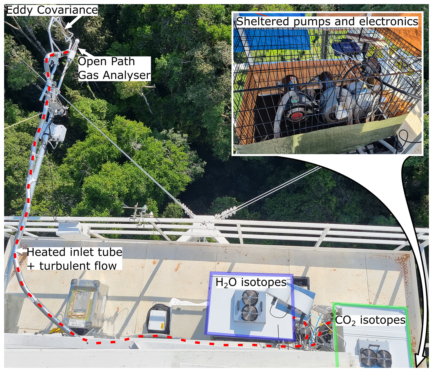
Figure 1 Picture of the isotopologue flux setup which was installed on the 54 m balcony of the ATTO tower in Central Amazonia, Brasil. The schematic overlay highlights the key components of the setup. The picture was taken by Oscar Hartogensis (oscar.hartogensis@wur.nl).

Data acquisition rates were 20 Hz for the anemometer and the OPGA, 10 Hz for the CO₂ isotope analyser, and 4 Hz for the H₂O isotope analyser. The EC data were processed using EddyPro version 7.06 (Fratini and Mauder, 2014) (from LI-COR Inc, Lincoln, USA), and the raw output was used for evaluation. The corrections applied include double rotation of the wind fields and density corrections according to the WPL method (Wilczak et al., 2001; Webb et al., 1980). The interquartile range (IQR) of the 30 min data evaluation periods was used as an outlier filter. Here, the isotopic compositions were filtered to retain 2 times the IQR, while 3.5 times the IQR was used for mole fraction and wind field data (described in Moonen et al. (2023)). Time synchronisation between the EC data and the isotope analysers was performed using time-lagged cross correlation on the CO₂ or H₂O mole fractions measured by both (Moonen et al., 2023). Additionally, the spectral correction method described in that manuscript is applied to correct for the spectral errors in the fluxes (see for example Fig. 4). An example of the workings of the spectral correction algorithm in co-spectral space is presented in Fig. A2. The calibration procedure for the isotope analysers during the CloudRoots Amazon22 campaign is described in Moonen et al. (2025a).

In this manuscript, we focus on the analysis of composite diurnal cycles of isotopic δ fluxes and net ecosystem flux compositions. Here, data from 8 August 2022 up to and including 20 August 2022 were used. Periods of instrument instability after startup, during maintenance, or during calibrations were removed. δ fluxes were furthermore filtered for outliers, where $\mathrm{15}\times {\mathrm{10}}^{-\mathrm{3}}$ ‰ m s⁻¹, $\mathrm{3.4}\times {\mathrm{10}}^{-\mathrm{3}}$ ‰ m s⁻¹, and $\mathrm{2.2}\times {\mathrm{10}}^{-\mathrm{3}}$ ‰ m s⁻¹ were the bounds for δD-H₂O, δ¹⁸O-H₂O, and δ¹⁸O-CO₂ fluxes, respectively. The uncertainties in the δ fluxes were determined through the spectral correction method, as described in Moonen et al. (2023). The uncertainty in the δ-flux-based net ecosystem flux signature (δ_…,F) was calculated by propagating the errors in both the net flux, and the δ fluxes. These uncertainties were limited to 30, 15, and 22 ‰ for δD, δ¹⁸O-H₂O, and δ¹⁸O-CO₂ respectively.

The second method we used to determine the isotopic composition of the net ecosystem exchange flux was the Miller-Tans method. Here, the uncertainties followed from propagating the error to the slope following York (1968) (Fig. A1). The threshold was set 5× smaller for δ_…,MT compared to δ_…,F, as the type of error is different.

Finally, the difference between the ET and atmospheric isotopic compositions (δ_ET−δ_atm) was limited to the ranges −20:70 ‰, and −16:26 ‰ for δD, δ¹⁸O-H₂O, respectively, and δ_NEE−δ_atm to $-\mathrm{75}:\mathrm{75}$ for δ¹⁸O-CO₂, in order to exclude outliers (see Figs. 3 and 5).

3.1 Ancillary data

Besides describing a representative diurnal cycle, we describe the isotopic state of the entire ecosystem in depth at 14:00. Our reason to select this period, is that fluxes are largest, the boundary layer has fully developed and the vegetation has reached isotopic steady state (Spiridonov and Ćurić, 2021; Farquhar and Cernusak, 2005). Here we use additional isotopic information from leaf and soil samples collected from 12 to 15 August 2022, which are described in Moonen et al. (2025a). For the leaves, samples taken from the canopy top (30 m) or the middle of the canopy between 12:00 and 16:00, were averaged to represent the 14:00 isotopic state. Soil samples were assumed not to vary in isotopic composition during the day. Here, the topsoil represents depths between 0–10 cm, and the deep soil depths between 40–100 cm. The isotopic composition of xylem water (δ_xyl) was approximated as the average of deep soil samples (40–100 cm depth, −3.83 ‰ for δ¹⁸O) and a water sample collected from a stream at approximately 70 m lower elevation (−4.86 ‰ for δ¹⁸O) which drains the plateau that hosts the ATTO site (see Fig. 6).

Averaged afternoon profile data of wind speed, relative humidity, CO₂ mole fractions, and temperature were used to accurately describe the environmental conditions near the leaves and the soil (González-Armas et al., 2025). Soil temperatures were measured at three locations, and the averaged 14:00 temperature was used for our analysis.

Finally, measurements of atmospheric δ¹⁸O-CO₂ compositions from flask samples were incorporated. In total, the data from 22 flasks were used to determine a representative 14:00 value. These were collected from air sampling inlets on the ATTO tower ranging from 50 to 312 m and collected during the early afternoon (12:00 and 16:00) on 14 and 15 August 2022. The data from the CO₂ isotope analyser could not be used to determine the background isotopic composition as it had a temperature dependent instability.

For the atmospheric compositions, δ fluxes, and ecosystem source compositions, the uncertainty associated with the 14:00 values represent the variability over the 13 composite days, expressed as the standard deviation (SD). In the case of leaf and soil samples, the uncertainty is the standard error of the mean (sem) of the samples. The uncertainty in δ_R is determined by propagating the sem in the topsoil water samples. For δ_P, we instead based its error on its sensitivity to $c_{\mathrm{i}}/c_{\mathrm{a}}$, where we assume that the ecosystem wide $c_{\mathrm{i}}/c_{\mathrm{a}}$ was determined with a 0.01 error (see Fig.8).

4 Results

4.1 H₂O δ fluxes and source compositions

Fig. 2 shows the composite diurnal cycle of the 57 m H₂O flux. We find a strong evapotranspiration flux during daytime, matching the period of solar irradiation (sunrise: 06:04, sunset: 18:04). Nighttime fluxes were close to zero, reflecting the reduction in turbulent transport and lack of available energy for evapotranspiration. The magnitude of the uncorrected H₂O flux derived using the water isotope analyser was 9.9 % smaller compared to the one derived with the conventional Open Path Gas Analyser (OPGA). Previously, water isotopologue flux studies have reported differences of tens of percent, indicating that we captured the high frequency contributions to the turbulent exchange flux reasonably well (Wahl et al., 2021; Moonen et al., 2023).

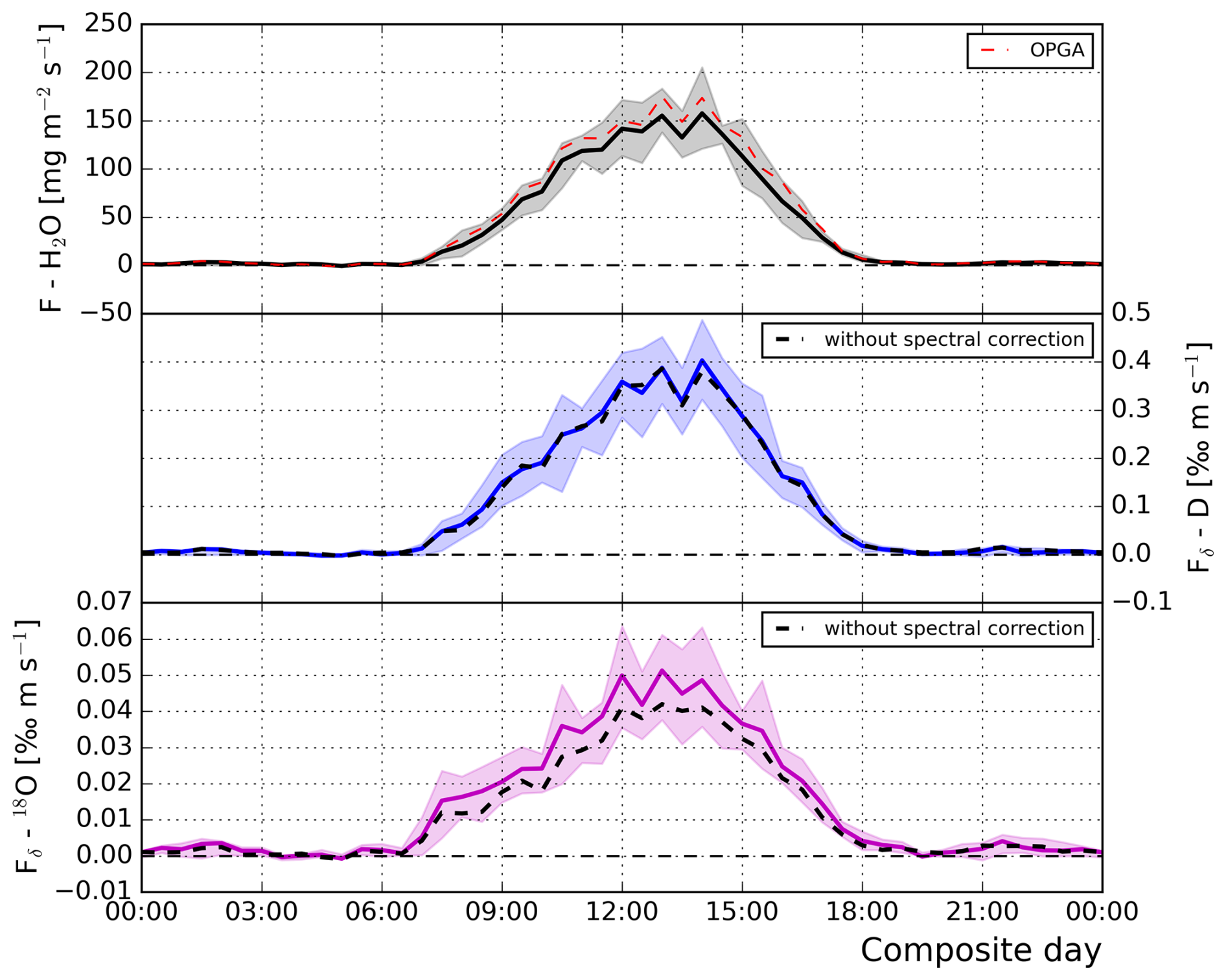
Figure 2 (top) Composite day 30 min average water flux derived using the closed path isotope analyser and an Open Path Gas Analyser (OPGA, shown in red). (middle) and bottom) Composite day 30 min average D and ¹⁸O δ fluxes derived using the water isotope analyser combined with the EC method. The dashed black lines show the data before correction of signal loss at high frequencies. The shaded areas indicate the 25 to 75 % quantiles of the 13 d contributing to the composite day.

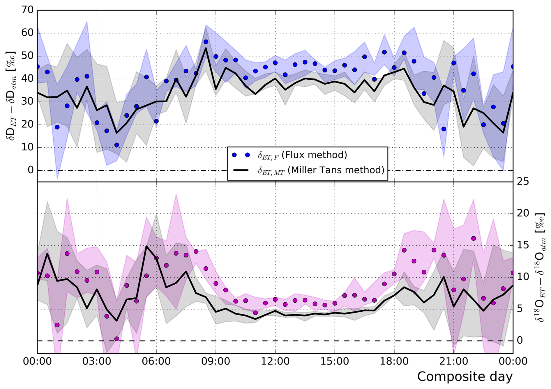
Figure 3 Composite day representation of 30 min average isotopic compositions of the net flux (δ_ET) derived using measurements performed with the water isotope analyser. The flux method composition (δ_ET,F) was derived using Eq. (4). Both the Miller-Tans and flux methods are described in Sect. 2.1. The shaded areas indicate the 25 % to 75 % quantiles of the 13 d contributing to the composite day.

The diurnal cycles of the δ fluxes have a very similar shape compared to the evapotranspiration flux. The variability over the days was somewhat larger however for the δ fluxes, as shown by the 25 % and 75 % quantiles (shaded). We applied the spectral correction method described in Moonen et al. (2023) to compensate for possible high frequency signal loss. Here, the cospectral power of frequencies lower than $\mathrm{8}\times {\mathrm{10}}^{-\mathrm{2}}$ Hz were used to estimate the cospectral power of the highest frequencies contributing to the flux. The black dotted line in the bottom two panels indicates the impact of this correction.

For δD, the magnitudes of the fluxes with and without spectral correction are effectively equal, indicating small high frequency signal attenuation. This finding was confirmed by the $w^{\prime }-{{\mathrm{H}}_{\mathrm{2}}\mathrm{O}}^{\prime }$ co-spectra related to the H₂O flux (see Moonen et al. (2023)). For δ¹⁸O, the spectral correction added 15.5 % to the flux, suggesting that there was a loss of high frequency signal for H${}_{\mathrm{2}}^{\mathrm{18}}$O. As attenuation is generally comparable for the various H₂O isotopologues, this was unexpected. Investigating the cospectra revealed that for δ¹⁸O, most frequencies contributed to the positive isotopologue flux as expected, but the highest frequency eddies had negative contributions (see Fig. A2). The reason for this phenomenon could not be identified.

Figure 3 shows the composite day overview of the isotopic composition of the net ET flux (δ_ET) derived using the Miller-Tans (δ_ET,MT) and Flux (δ_ET,F) methods. For δ¹⁸O as well as for δD, we find that δ_ET is always enriched compared to δ_atm. During nighttime, the isotopic composition of the net flux is highly variable over time for both species. For the flux method, this is directly related to the very small (near-zero) water vapour and δ fluxes shown in Fig. 2. Equation (4) clarifies that a large uncertainty for the fluxes leads to poor estimates for δ_ET,F. For the Miller-Tans method, the small perturbations in isotopic compositions and mole fractions associated with stable nighttime conditions also lead to large uncertain δ_ET,MT estimates. Moreover, these stable conditions suppress mixing, which leads to horizontally heterogeneous conditions in the forest, which results in variability between the different nights (Botía et al., 2020). During daytime, the isotopic compositions of the net exchange are instead well defined, with little variability between the contributing days.

From 10:00 to 17:00 we find that δ_ET is quite constant, with a 40 ‰ enrichment for δD, and a 5 ‰ enrichment in δ¹⁸O compared to the ambient atmospheric water vapour. This is consistent with the evapotranspiration of comparatively enriched water from the ecosystem to the atmosphere. For both δ¹⁸O and δD we observe that net flux compositions obtained with the flux method (δ_ET,F) are more enriched than those derived from the Miller-Tans method (δ_ET,MT) during the same period. On average, the difference is 6.4 ‰ for δD and 1.9 ‰ for δ¹⁸O. The causes of this difference and the implications for the partitioning of ET are discussed in Sect. 5.1.

4.2 CO₂ δ fluxes and net flux compositions

In Fig. 4, the CO₂ flux and corresponding isotopologue flux measurements are summarised. The NEE flux in the top panel indicates strong negative CO₂ flux during daytime, indicating photosynthetic uptake. Immediately after sunrise, however, a small positive CO₂ was observed. We interpret this positive flux to be related to the nighttime respiratory flux, which feeds CO₂ into the nocturnal boundary layer (Dupont et al., 2024). As this layer is stably stratified due to the radiative cooling of the surface, the CO₂ is trapped in the atmospheric layer below the 57 m measurement height, which includes the entire canopy. When the stability is broken after sunrise, this accumulated respiratory CO₂ is transported upward to the boundary layer and across the measurement location.

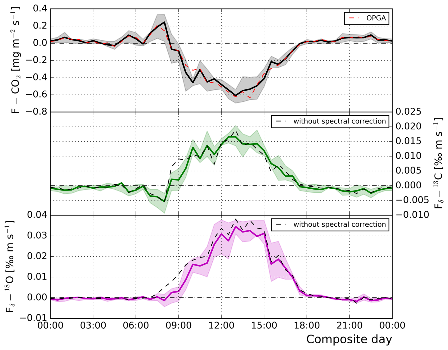
Figure 4 (top) Composite day 30 min average CO₂ fluxes derived using the closed path isotope analyser and an Open Path Gas Analyser (OPGA, shown in red). (middle) and (bottom) Composite day 30 min average ¹³C and ¹⁸O δ fluxes derived using the CO₂ isotope analyser combined with the EC method. The dashed black lines show the data before correction of signal loss at high frequencies. The shaded areas indicate the 25 % to 75 % quantiles of the 13 d contributing to the composite day.

The fluxes derived with the closed path CO₂ isotope analyser compare very well to the OPGA, without any notable signal loss. The δ fluxes can thus also be expected to be resolved well. In terms of diurnal pattern, the δ flux of δ¹³C is a mirror image of the NEE flux, including the release of trapped nocturnal respiration after sunrise. During nighttime, both the ¹³C δ flux and NEE show a near continuous respiration flux, which is unlike the near zero fluxes for ET and δ¹⁸O-CO₂.

The ¹⁸O-CO₂ δ flux has a diurnal pattern which is more similar to the ET and water isotope δ fluxes. The main difference is the time from which the flux becomes positive, which is delayed by 1.5 h for ¹⁸O-CO₂. The effect of the spectral corrections is similar for both δ¹³C and δ¹⁸O, although somewhat stronger for δ¹⁸O. Here, the method described in Moonen et al. (2023) was primarily used to correct for instrument instabilities at frequencies lower than $\mathrm{9}\times {\mathrm{10}}^{-\mathrm{4}}$ Hz. Since the instrument instability increased the variability of the isotopic signals, and thus increased the magnitude of the flux, the spectral correction method leads to smaller δ fluxes for CO₂.

Figure 5 shows the composite day overview of the isotopic composition of the NEE flux (δ_NEE) derived using the flux (δ_NEE,F) method. While for H₂O the source composition can be interpreted as the composition being mixed into the atmosphere, this is not as self evident for CO₂. This is because the net exchange of CO₂ transitions from positive values during nighttime (R) to negative values during daytime (P and R). Following Eq. (4), the isotopic composition of the net ecosystem exchange flux must be interpreted in line with the sign of the flux. Thus, during daytime it represents the isotopic composition of the (negative) uptake flux. For δ¹³C, we find uptake flux compositions which are depleted by 20 ‰ compared to the atmosphere during both day and nighttime (see Fig. 5). At nighttime, this represents the signature of respiration from decomposing organic matter. During daytime, the isotopic signature of the assimilated CO₂ is measured, which reflects the preferential uptake of depleted carbon by C3 vegetation (trees). Note that during daytime, contributions from the depleted respiration flux are also present.

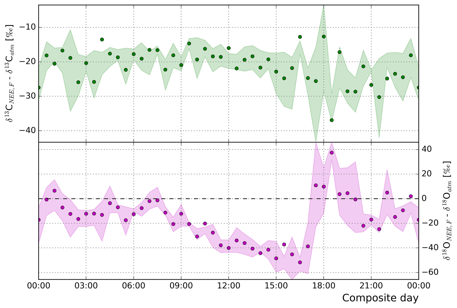
Figure 5 Composite day representation of 30 min average isotopic compositions of the net CO₂ flux (δ_NEE) derived using the CO₂ isotope analyser. δ_NEE was derived using the flux method (δ_…,F), following Eq. (4). The deviations from the atmospheric background are plotted. The shaded areas indicate the 25 % to 75 % quantiles of the 13 d contributing to the composite day.

The ¹⁸O isotopic composition of the NEE is approximately −15‰ lower than the one of ambient atmospheric CO₂ during the night according to the bottom panel of Fig. 5, and this difference steadily increases to −50 ‰ in the late afternoon. As explained above, this is an apparent fractionation that does not represent the fractionation associated with physical CO₂ uptake, but it is due to back diffusion of CO₂ after isotopic exchange with water. Thus, it is necessary to consider the δ¹⁸O of the water with which CO₂ equilibrates in the leaves. During nighttime, leaf water is strongly depleted in δ¹⁸O compared to daytime, which leads to respired CO₂ being depleted in δ¹⁸O compared to atmospheric CO₂ (see Table A2). This δ¹⁸O depletion is indeed observed at night. During daytime, δ¹⁸O in leaves gradually increases due to evaporative enrichment. As a consequence, the CO₂ molecules that exchange isotopes with water and are partially assimilated must also be comparatively enriched in ¹⁸O.

So, why do we then observe a continuous depletion in δ¹⁸O_NEE compared to the atmospheric δ¹⁸O value? This is due to the net uptake of CO₂ during daytime (negative CO₂ flux), combined with the substantial diffusion of equilibrated and thus isotopically enriched CO₂ back into the atmosphere (Adnew et al., 2020). The latter effect is dominantly responsible for affecting the atmospheric isotopic composition of CO₂. However the (apparent) composition of the net uptake flux is what is determined. In our case, this net uptake flux seemingly strongly favours ¹⁶O, as it enriches the atmosphere in ¹⁸O, which results in a negative ${\mathit{\delta }}_{\mathrm{F}}^{\mathrm{18}}$O (Farquhar and Lloyd, 1993; Adnew et al., 2021). The strongly depleted δ¹⁸O composition of the daytime carbon flux is thus a consequence of the enrichment of the atmosphere due to back-diffusion. Other researchers have found similar diurnal cycles for δ¹⁸O to the ones we present in the bottom panel of Fig. 5 (for example Sturm et al. (2012), their Fig. 9b (dry conditions)). The apparent fractionation effect during photosynthetic uptake is further explored in Sect. 4.4.

During the transition to nighttime respiration, leaf water remains temporarily enriched in ¹⁸O, which leads to the enriched source signature visible between 17:30 and 20:00. Here, the NEE and δ flux are near zero, leading to more variability between the days, as indicated by the shaded area. Compared to the highly variable nighttime source compositions for H₂O, the source compositions for the CO₂ isotopes are better defined during the night. This is because there are still significant net exchange fluxes and isotopologue fluxes during nighttime. During the morning, the transition between the respiration peak and the onset of photosynthesis is more abrupt than during the evening transition, which allows for the source compositions to be well estimated comparatively during that time. During the evening transition around 18:00, when the sign of the net exchange flux changes to the respiration dominant nighttime, some erratic NEE isotopic signatures are also found in ¹³C.

4.3 The H₂O isotopic state

We investigated the isotopic signatures of H₂O in water reservoirs that are relevant for the exchange of water (and CO₂) around the ATTO tower. Here, we describe the isotopic compositions within the soil, canopy, and atmospheric reservoirs, as well as the isotopic composition of the associated vertical water vapour flux as measured above the canopy. The isotopic compositions of reservoirs which were not measured directly and of individual gross fluxes were then derived following Sect. 2. The result is a coherent and connected isotopic cascade throughout the Amazonian ecosystem. We describe the 14:00 case which ensures that the atmospheric boundary layer (ABL) is fully developed and that isotopic steady-state has set in. To limit the effect of the sub-diurnal and inter-diurnal variability, the 14:00 case was derived from a 13 d composite diurnal cycle.

Table 1 specifies the typical environmental conditions at 14:00 at the ATTO site. These variables are key inputs for describing the isotopic H₂O and CO₂ balances. For a rainforest, the RH of 58 % within the canopy is relatively low. Note that the campaign took place during the dry season, and that only two significant rain events took place during the 13 d campaign. In addition, temperatures are highest around 14:00, contributing to a reduced RH. As a consequence, the vegetation limits evaporation by reducing its stomatal apertures, resulting in a comparatively high stomatal resistance R_s during this time. In line with this, the $c_{\mathrm{i}}/c_{\mathrm{a}}$ is at a daily low at 14:00.

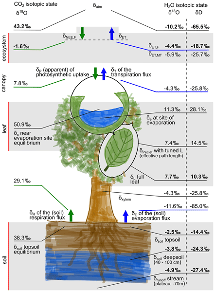
The right hand side of Fig. 6 specifies the isotopic state of water in all the relevant reservoirs for both δD and δ¹⁸O. Here, we combined atmospheric observations, flux measurements, and leaf and soil level measurements (also see Table A1). Two flux pathways are highlighted by which water vapour is fed to the atmosphere: (soil) evaporation and transpiration, respectively. Here, the transpired water (δ_T) is enriched compared to the atmospheric reservoir (δ_atm), whereas the evaporated water δ_E is depleted compared to δ_atm. This difference is key to resolve, as it allows us to partition the net ET flux into the components E and T in Sect. 4.5.

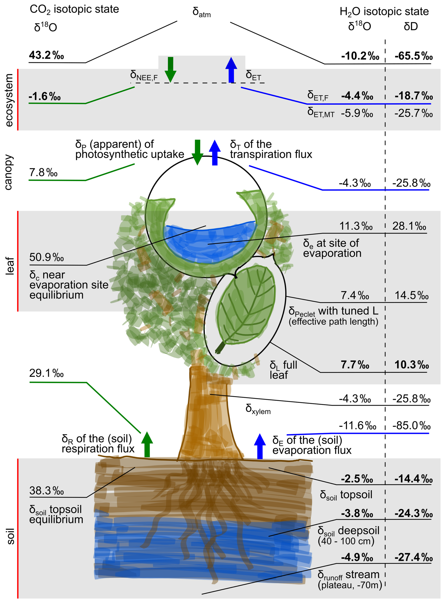
Figure 6 Overview of the CO₂ and H₂O isotopic state of the Amazon rainforest ecosystem, representative for the average 14:00 conditions at the ATTO site during the 13 d CloudRoots-Amazon22 field campaign. Bold font indicates that the variables were derived from measurements (also see Sect. 3.1). The vertical text highlights the scale which a certain set of variables grouped by shade/no-shade represents. The uncertainties associated with the values are provided in Tables A2 and A1 of the Appendix, if available.

Ultimately, the source water of both evaporation and transpiration is the same, namely precipitation. While there is some seasonal variability in the isotopic composition of precipitation, with the wet season feeding more depleted water to the ecosystem, this will not impact our 13 d measurement campaign (Zhiña et al., 2022). The isotopic composition of topsoil water (δ_soil) is determined by the composition of recent precipitation and the accumulated effect of the evaporative enrichment of the near-surface water reservoir due to Rayleigh fractionation. The latter effect results in the topsoil water to be more enriched compared to the water below (see Fig. 6). Compared to δ_soil, the evaporated water δ_E is strongly depleted due to the preferential evaporation of HHO compared to HDO (Horita and Wesolowski, 1994).

As explained above, the isotopic composition of transpiration (δ_T) is assumed to be identical to δ_xylem because of mass conservation (Dongmann et al., 1974). As a result, the isotopic composition of transpired water vapour (δ_T) is much more enriched than δ_E. The Craig-Gordon model (Eq. 7) allows to determine the isotopic composition of liquid water at the exchange site (δ_e) that is required to supply these high values of δ_T. The results representing our study case are shown in Fig. 6: δ¹⁸O_e is 15 ‰ higher than δ¹⁸O_xylem, while δD_e is more than 50‰ more enriched than δD_xylem. Liquid water samples of entire leaves (δ_L), which comprise both the leaf veins and the leaf lamina, bridge the composition of the enriched evaporation sites, and the comparatively depleted δ_xylem source water (Cernusak et al., 2016). Given that we know both of these end members, and the leaf water isotopic composition, we are able to estimate a value for the Péclet number using Eq. (10). Since we also know the transpiration rate from the partitioning result, we can subsequently solve for L in Eq. (9), which is the effective path length over which water transport in leaves takes place. This results in a value of L=10 mm, should be seen as a representative value for the entire footprint of the EC system, and accounts for transport through both the larger leaf veins and the smaller leaf capillaries. This value for L was associated with Péclet numbers of 0.61 for δ¹⁸O, and 0.6 for δD. Table A1 specifies the important intermediate steps in the isotopic cascade, and also provides the uncertainties for some of the variables.

4.4 The CO₂ isotopic state

The left hand side of Fig. 6 specifies the 13 d averaged 14:00 isotopic state for δ¹⁸O-CO₂. Similar to H₂O, two flux pathways are highlighted which together determine NEE, namely the (soil) respiration flux (R) and the photosynthetic assimilation flux (P). Importantly, the isotopic exchange of ¹⁸O-CO₂ is controlled by the isotopic composition of H₂O throughout the ecosystem, which means that tight links between the left and right hand sides of Fig. 6 exist.

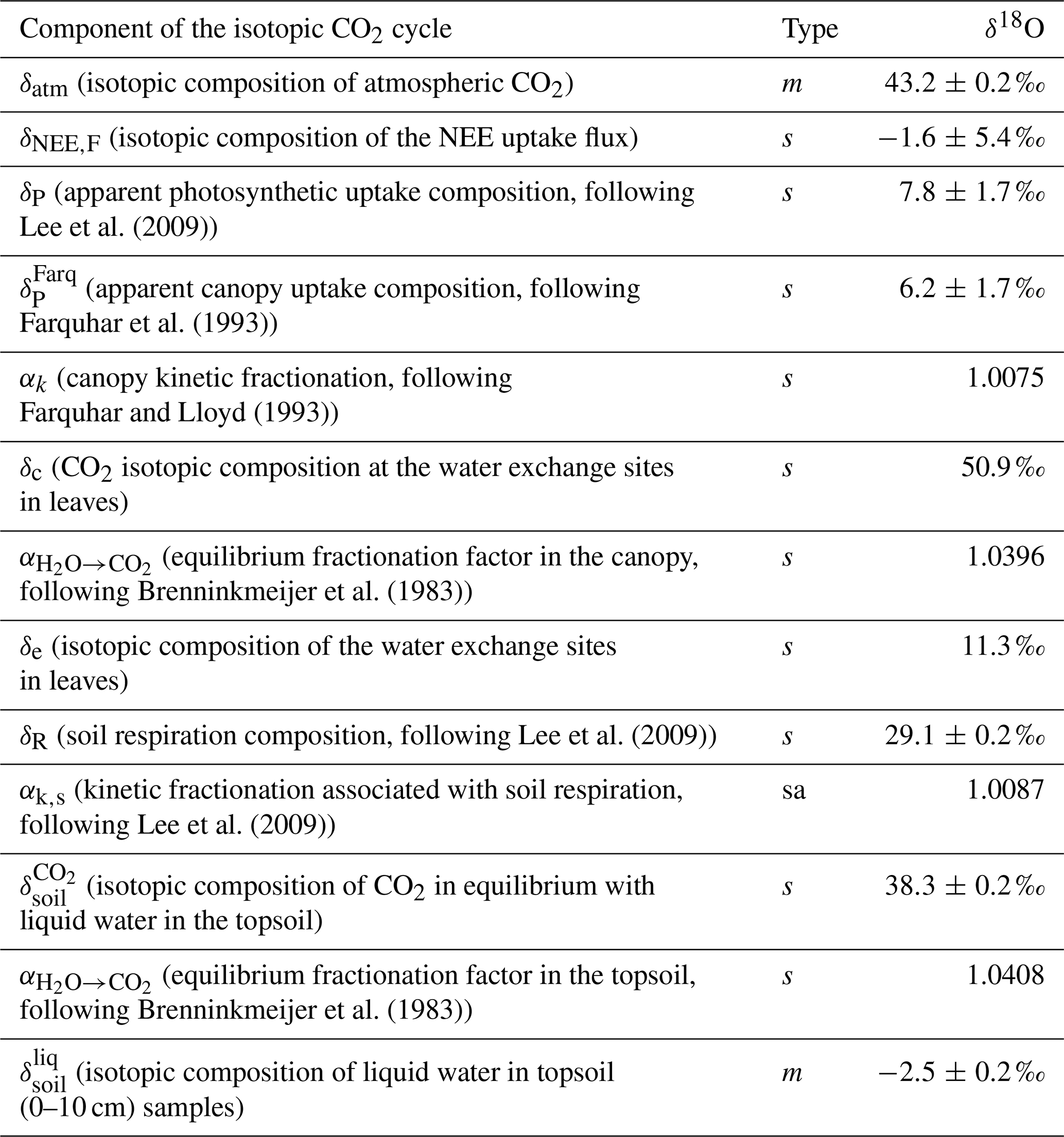
The isotopic composition of assimilated CO₂ (δ_P) is apparently strongly depleted in ¹⁸O compared to δ_atm. This is a particularly important and counter-intuitive effect in the δ¹⁸O-CO₂ cascade, and it results from the isotopic exchange between CO₂ and H₂O in the mesophyll of leaves. Oxygen isotopes are exchanged so quickly between CO₂ and H₂O that the isotopic composition of CO₂ in the stomata is generally believed to be in isotopic equilibrium with the H₂O at the site of exchange (Farquhar and Lloyd, 1993). This means that the δ¹⁸O-CO₂ in the stomata is decoupled from the isotopic composition of ambient CO₂, and in our case enriched (see δ_c). As mentioned above, part of this isotopically enriched CO₂ diffuses back through the stomata and isotopically enriches the atmospheric reservoir. The net effect of the CO₂ exchange through the stomata is (photosynthetic) uptake however, so the atmosphere close to the leaf does have lowered CO₂ mole fractions. The combination of the net uptake and the back-diffusion of ¹⁸O- enriched CO₂ makes it seems as though ¹⁶O-CO₂ is apparently assimilated faster than ¹⁸O-CO₂. It is important to realize that this is not what happens physically, but that an apparent fractionation effect takes place (Adnew et al., 2020).

δ_P-δ_atm indicates the strength of the apparent fractionation effect, which is −35 ‰. This difference is larger than what might be expected given the isotopic composition near the exchange sites (δ_e) in the mesophyll (δ_c-δ_atm) of about 8 ‰. In Sect. 4.5 we detail how this amplification emerges in relation to the $c_{\mathrm{i}}/c_{\mathrm{a}}$ ratio, which determines the relative strength of the back-diffusion. This effect turns out to be key for partitioning NEE. In contrast to δ_P, the isotopic composition of respired CO₂ (δ_R) is only weakly depleted relative to δ_atm (−14.1 ‰).

The source signature of the soil respiration flux (δ_R) is primarily affected by equilibration with the soil water isotopic composition. Any CO₂ in the soil, whether it has been locally respired or invaded from the atmosphere, equilibrates with topsoil H₂O_l (${\mathit{\delta }}_{\mathrm{soil}}^{\mathrm{liq}}$, Wingate et al. (2009)). During the subsequent diffusion from the soil into the atmosphere, the CO₂ from the soil (${\mathit{\delta }}_{\mathrm{soil}}^{{\mathrm{CO}}_{\mathrm{2}}}$) undergoes kinetic fractionation (Table A2). This results in a depletion of the isotopic composition of the respiration flux (δ_R) compared to ${\mathit{\delta }}_{\mathrm{soil}}^{{\mathrm{CO}}_{\mathrm{2}}}$. In addition, invasion of CO₂ into the soil and subsequent back diffusion into the atmosphere has a depleting effect. However, as the concentration of CO₂ in a tropical rain forest soil is much higher then in the atmosphere, this effect is comparatively small (Hashimoto et al., 2004).

In total, the enriching effect of δ_P on δ_atm is larger than the depleting effect of δ_R, which results in the net positive δ¹⁸O-flux we observe in Fig. 4. In line with this, and given that the NEE flux is negative, the isotopic composition of this flux (δ_NEE,F) is depleted compared to the atmospheric background. Using our measurements and Eq. (4), δ_NEE,F was determined as −1.6‰. This is lower than both the canopy and the soil flux end-members δ_P and δ_R, which can seem illogical. This is, however, a mathematical effect of attributing the depletion associated with both gross fluxes to one, smaller, net flux. In fact, we show below that the derived value of δ_NEE,F does allow for the flux partitioning equations to be solved (Sect. 4.5), and it is in line with previously measured values by, for example, Griffis (2013), who found a δ_NEE,F of −10.5 ‰ above a soybean field.

4.5 Net ecosystem flux partitioning

The values established in previous sections can be used to partition the measured net ecosystem exchange fluxes NEE for CO₂ and ET for H₂O into the individual gross flux components according to Eq. (2). δ_ET was taken as the average of the values determined from the direct flux measurements δ_ET,F and the Miller-Tans mass balance approach δ_ET,MT. δ_E was assumed to equal ${\mathit{\delta }}_{\mathrm{soil}}^{\mathrm{vap}}$, as described in Sect. 2.2, and δ_T was represented by δ_xyl (see Sect. 2.2). Using the average of the partitioning results derived from δD and δ¹⁸O, we find that the transpiration flux (T) contributes 95.5 % to ET at 14:00 on average (Fig. 7). A dominant contribution of T is expected given the high uptake of radiation by the canopy crown and resulting shading in the understory (González-Armas et al., 2025). The 4.5 % contribution from soil evaporation flux (E) is an important finding, as few studies have attempted to estimate the soil contributions, and it is assumed in many studies that no soil evaporation takes place at all (Belk et al., 2007; Schellekens et al., 2000; Malhi et al., 2002). Note that ET partitioning using δD only results in E=0, as δD_ET is even more enriched than δD_T according to our measurements.

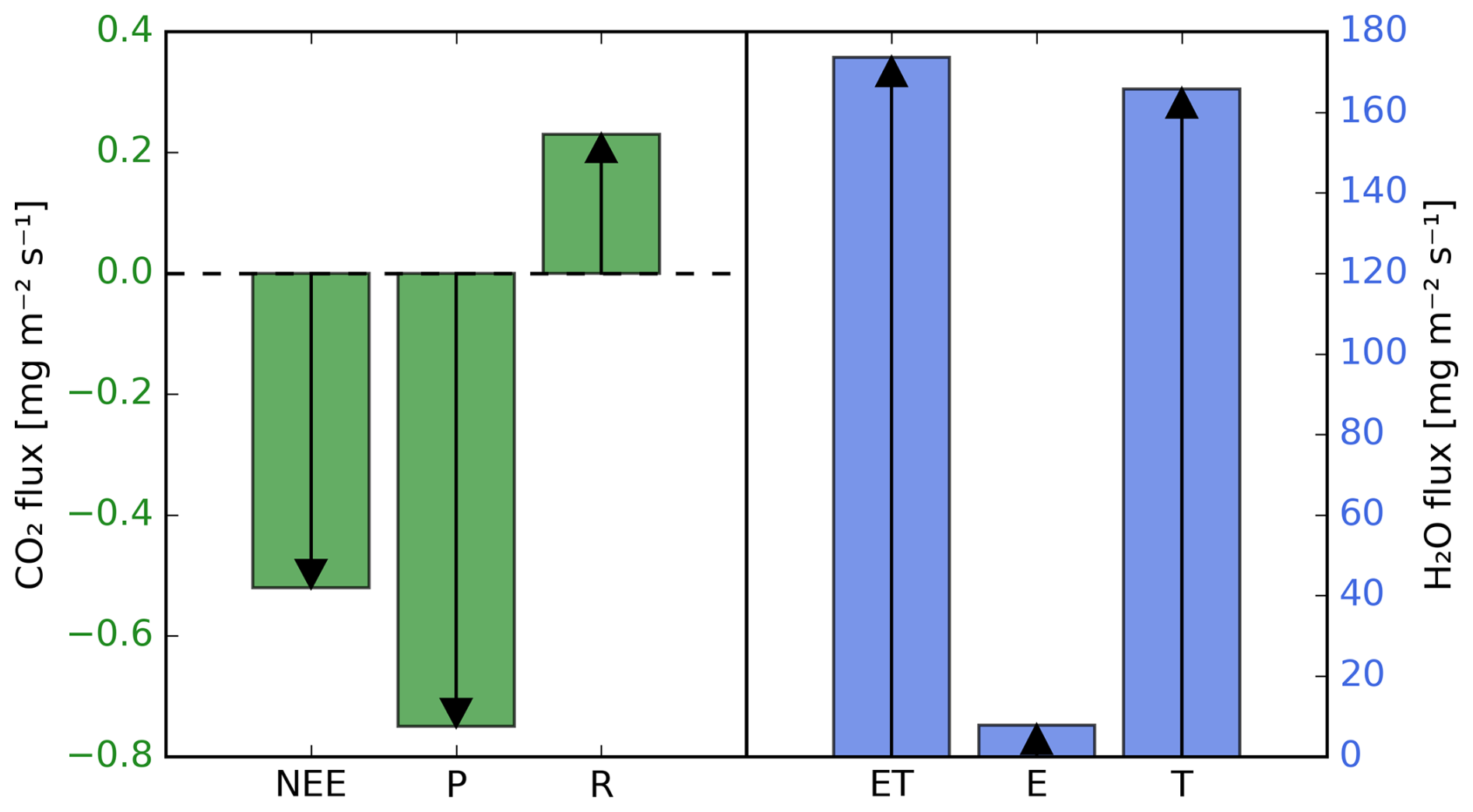
Figure 7 Results of the partitioning of the net ecosystem exchange fluxes NEE and ET based on the 13 d composite 14:00 isotopic state, following Eq. (2). For NEE, the ¹⁸O-CO₂ isotope was used following the approach described in Sect. 2.3. For ET, the average of the partitioning results derived from δD and δ¹⁸O is shown (see Sect. 2.2).

For the NEE flux, the partitioning suggests that P is 144 % of NEE, which is compensated by an R of −44 % of NEE (Fig. 7). We found that this result was strongly dependent on the component δ_P, which is the apparent isotopic composition of P. Given its origin from CO₂ back-diffusion, the strength of δ_P depends on $c_{\mathrm{i}}/c_{\mathrm{a}}$. For the value we used ($c_{\mathrm{i}}/c_{\mathrm{a}}=\mathrm{0.79}$) we find δ_P=7.8 ‰. To interpret δ_P, it helps to consider $c_{\mathrm{i}}/c_{\mathrm{a}}$ as describing a balance of opposing diffusive fluxes ($F_{\mathrm{out}}/F_{\mathrm{in}}\propto \frac{c_{\mathrm{i}}/c_{\mathrm{a}}}{\mathrm{1}-c_{\mathrm{i}}/c_{\mathrm{a}}}$). The value of 0.79 means that for every CO₂ molecule being assimilated, roughly 4 CO₂ molecules diffuse back into the atmosphere. This illustrates that while the enriching effect on the atmosphere is not large per back-diffusing molecule (see Fig. 6), the effect is leveraged 4 fold when interpreting it as a fractionation effect resulting from photosynthetic uptake alone. In Sect. 5 we explore the sensitivity of the partitioning result to this uptake fractionation leveraged by $c_{\mathrm{i}}/c_{\mathrm{a}}$.

The uncertainty in the partitioning result is determined by the uncertainties in the net ecosystem fluxes (ET and NEE), the isotopic end-members (δ_E, δ_T, δ_R, and δ_P), and the derived isotopic composition of the net ecosystem exchange fluxes (δ_ET and δ_NEE). Here, the uncertainties in the isotopic components can be assumed to be largest. In Tables A1 and A2 we provide the estimated errors in all of these isotopic components. Note however, that the various types of errors are not directly comparable. For example, the large uncertainties in δ_ET and δ_NEE, which indicate the variability (SD) in these variables over the 13 composite days, are likely smaller than the end-member compositions (sem) when considering the instantaneous 14:00 afternoon case we analyse (see Sect. 3.1). As a result, we have not explicitly determined uncertainties for the partitioning results.

5 Discussion

We have used in-situ measurements of CO₂ and H₂O isotopologue fluxes far above the top of the canopy in the Amazon forest (57 m) to partition the net ecosystem fluxes of both NEE and ET into their individual components. This was possible because we could describe the complete isotopic state of δ¹⁸O in both CO₂ and H₂O throughout the ecosystem by making use of additional isotopic information from leaf and soil samples. Here, we have demonstrated that the isotopic states at the evaporative sites in the leaves – where CO₂ and H₂O isotopic cascades intersect – are physically consistent between the two species. Our results give confidence that isotopologue flux measurements can provide reliable ecosystem scale partitioning results.

5.1 Ecosystem source compositions

As shown above, we have used high frequency isotope measurements to determine the isotopic composition of the ecosystem flux (δ_ET and δ_NEE). For δ_ET, two estimates were used and compared: one using the measured δ flux (δ_ET,F) and the other one using the Miller-Tans δ_ET,MT method. We found that δ_ET,F produced systematically more enriched values, where δD was 6.4 ‰ more enriched and δ¹⁸O was 1.9 ‰ more enriched compared to δ_ET,MT. Griffis et al. (2007) also compared the δ_ET,F to a mixing model method, however for δ¹³C of CO₂. They found that δ_ET,F was ≈5 ‰ more enriched, which in their case meant closer to δ_a, than δ_ET,MT. They attributed this systematic effect to footprint differences. δ_ET,F indeed represents local exchange in the footprint area of the isotope and the net ecosystem flux measurements, while δ_ET,MT can also be influenced by other up-wind exchange processes, which affect the measured atmospheric compositions (see Fig. A1). It is not clear, however, why up-wind exchange would be much different compared to local exchange, given the homogeneity and vast scale of the Amazon rainforest ecosystem surrounding the ATTO site.

We suggest that differences between δ_…,F and δ_…,MT should be further investigated to determine which method is more appropriate for determining the isotopic composition of the ecosystem flux. For now, we speculate that the estimate from δ_…,F will be more reliable because (1) the footprint better matches the flux and in-ecosystem measurements we took, and (2) because the Miller-Tans method is subject to stringent assumptions which are not underlying the flux method. Here, especially the two end-member mixing assumption is likely violated, as vapour sources from an ecosystem are not isotopically uniform, but highly variable in composition (Miller and Tans, 2003; Griffis et al., 2010; Cernusak et al., 2016).

5.2 The sensitivity of ecosystem partitioning to local sampling

Determining flux partitioning at the ecosystem scale is important for linking the understanding of leaf and canopy scale processes to the scales relevant for remote sensing and modelling purposes (Gentine et al., 2019; Vilà-Guerau de Arellano et al., 2023). It is important to realize that leaf and soil water isotopic composition measurements are always necessary to determine the end members for isotopic partitioning. In addition, $c_{\mathrm{i}}/c_{\mathrm{a}}$ ratios need to be known, and they are usually determined with dedicated (and labour intensive) leaf gas exchange measurements (González-Armas et al., 2025). While we attempted to capture the variation across space and species in these variables, it is challenging to obtain a subsample that is truly representative for the entire ecosystem. Moreover, such measurements are labour intensive. Once a high temporal resolution isotopologue flux system is in place, this may be the least time consuming component of the flux partitioning system. Therefore, we consider the necessity of detailed leaf and soil scale measurements to be the major obstacle for more wide spread implementation of isotopic ecosystem scale flux partitioning.

Replacing detailed leaf and soil scale measurements with assumptions or approximations based on environmental variables is appealing for simplifying isotopic ecosystem scale flux partitioning. For example, the $c_{\mathrm{i}}/c_{\mathrm{a}}$ ratio is regularly assumed to be 0.7 (Farquhar et al., 1989a). Alternatively, its value can be approximated using the stomatal conductance and the water vapour pressure deficit (Ronda et al., 2001). However, we find that the isotopic end-member δ_P is highly sensitive to the $c_{\mathrm{i}}/c_{\mathrm{a}}$ ratio, which makes us believe that approximations are likely insufficient for deriving reliable partitioning values. Even with the intensive $c_{\mathrm{i}}/c_{\mathrm{a}}$ monitoring during CloudRoots-Amazon22, described in González-Armas et al. (2025), we are left with some uncertainty regarding an appropriate $c_{\mathrm{i}}/c_{\mathrm{a}}$ ratio. Figure 8 indicates how this uncertainty propagates to the determination of δ_P, and what the consequences are for the NEE partitioning result.

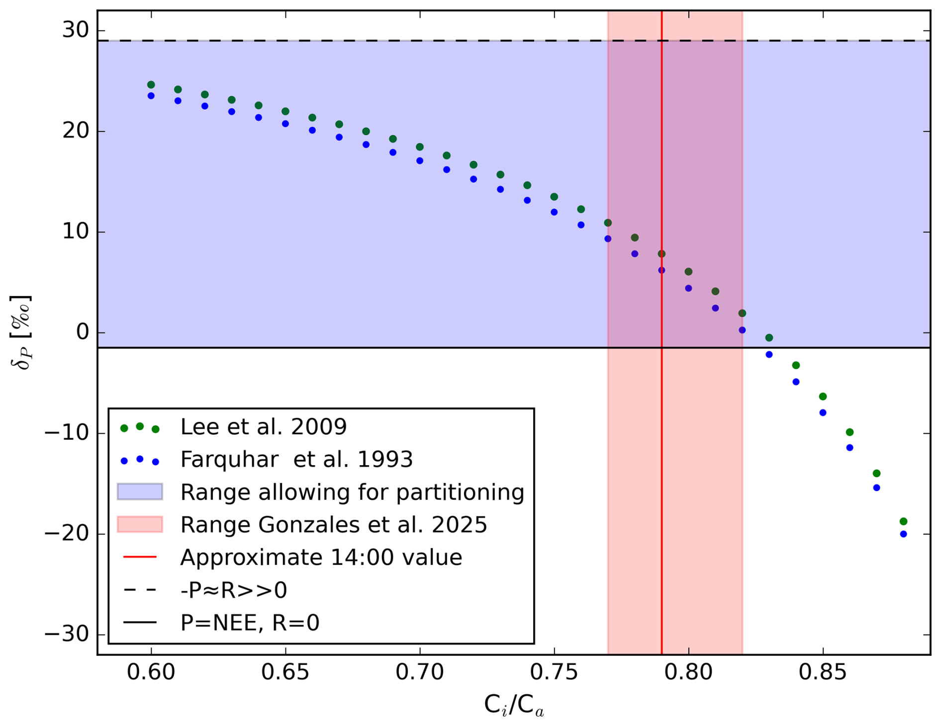
Figure 8 Simulated sensitivity of δ_P to the $c_{\mathrm{i}}/c_{\mathrm{a}}$ ratio following the original mathematical formulations of Farquhar et al. (1993) and the formulation of Lee et al. (2009) in which the incomplete equilibration between H₂O and CO₂ is considered (Eq. 13. The red line and shading indicate the average value and total observed range of $c_{\mathrm{i}}/c_{\mathrm{a}}$ at 14:00 (González-Armas et al., 2025). The horizontal black lines indicate the upper and lower limits of δ_P determined at 14:00 from a 13 d composite, for which a partitioning result based on Eq. (2) can be found (blue range) given the isotopic composition of NEE (${\mathit{\delta }}_{\mathrm{NEE},\mathrm{F}}=-\mathrm{1.6}$ ‰) and of the soil respiration end-member (δ_soil=29.1 ‰).

For our observed value of $c_{\mathrm{i}}/c_{\mathrm{a}}=\mathrm{0.79}$, Fig. 8 indicates that an isotopic composition of the canopy uptake flux (δ_P) is found which allows for the partitioning of NEE. However, the upper bound of the possible $c_{\mathrm{i}}/c_{\mathrm{a}}$ range would result in a δ_P close to the solid horizontal line, which indicates the limit of possible partitioning results, leading to a respiration flux of near zero. The lower bound of the possible $c_{\mathrm{i}}/c_{\mathrm{a}}$ range, 0.77, which is only smaller by 0.05, would instead suggest a large R (−69 % of NEE), compensated by a strong P uptake flux (169 %). The exact value of the ecosystem wide $c_{\mathrm{i}}/c_{\mathrm{a}}$ is thus important to know. Note that the daytime averaged $c_{\mathrm{i}}/c_{\mathrm{a}}$ is approximately 0.86, which does not allow for partitioning at all. To describe the ecosystem exchange, it is thus essential to resolve the diurnal cycle of variables like $c_{\mathrm{i}}/c_{\mathrm{a}}$ with measurements, which allows for the diurnal dynamics to be taken into account appropriately.

5.3 Water isotopic (steady-) state

For the H₂O isotopes, the assumption of isotopic steady-state is important and much discussed (Farquhar and Cernusak, 2005; Barbour et al., 2017; Yakir and da Silveira Lobo Sternberg, 2000). This assumption emerges from the principle of mass conservation, and implies that during continuous transpiration, a balance is established between the isotopic composition of the water taken up by a plant, and the water vapour transpiring into the atmosphere. This directly relates to the strong isotopic enrichment of the water at the evaporation sites in the leaves, which leads to and maintains the enrichment of the transpiration (vapour) flux. While this assumption is adequate for longer timescale (1 month) analysis, it has been shown to be problematic at short timescales (<1 d), where irregularities due to buffering and fast fluctuations in environmental conditions are observed (Cernusak et al., 2016). In our analysis we have used the steady-state Craig-Gordon model. For the 14:00 case, we do not expect the steady-state assumption to be violated, as this is the time of day where enough water has been processed through the plant, and is being transpired, for steady-state to set in (Griffis, 2013). However, if we expanded our analysis to the entire diurnal cycle – where during the night transpiration is small and the leaf evaporation sites are not enriched – the steady-state assumption would most likely not be adequate.

Non-steady-state Craig-Gordon models allow to describe diurnal dynamics better than steady state models, and would therefore be preferred for ecosystem scale flux partitioning(Craig and Gordon, 1965). However, they require independent estimation of the isotopic composition of transpired water (δ_T), without assuming that this composition is equal to the source water (δ_xylem), as we have done under the steady-state assumption. In natural ecosystems, δ_T is not only difficult to measure, it is also complex to estimate independently. Ideally, the isotopic composition of the water at the evaporation site (δ_e) would be known, so that δ_T can be solved for reliably. Direct sampling of δ_e is impossible however, as the actual sites of evaporation are microscopically small. Instead, water samples from complete leaves or leaf lamina might be used to estimate δ_e by taking into account the Péclet effect. The limit here is that the magnitude of the Péclet effect is highly dependent on hard to determine variables like the effective path length (L, see Eq. 9). Estimates for this variable vary considerably between experiments and species (Lai et al., 2008). The value L=10 mm that we determined for the 14:00 steady state of the 13 d composite, is in line with previously reported values by for example Barbour and Farquhar (2004), who found L=8 mm. While steady-state leaf water assumptions are thus known to be inadequate, the increased complexity of non-steady-state models is hard to take into account in natural ecosystems, posing a limit for applying the ecosystem flux partitioning technique using isotope information to the entire diurnal cycle.

The isotopic steady-state assumption is not applicable to soils due to the comparatively large size of the water reservoir in contact with the atmosphere (Wingate et al., 2009). This results in diffusion of enriched water from the evaporation sites back into the topsoil water pool. Over time, this results in the gradient we illustrate in Fig. 6, where the topsoil becomes enriched compared to the deep soil water. This enrichment can be expected to have a limited diurnal cycle, which allows for topsoil water samples to be used to estimate δ_E for the entire day. The topsoil water enrichment we find during CloudRoots-Amazon22 is very small, with a gradient in δD of 8.6 ‰. Canet-Martí et al. (2023) instead find gradients in δD reaching 40 ‰ in agricultural fields. The resetting of the gradient by regular precipitation in the Amazon could in part explain this large difference. On top of this, the strong shading from the rainforest canopy, and leaf litter, which limit solar irradiance and thereby E, contributes to the small soil water isotopic gradients in the Amazon.

5.4 Broader perspective

The work presented in this chapter shows that isotopic flux partitioning is possible and offers insight into the individual gross fluxes. Further implementation of the method is limited by (1) the requirement for local scale sampling measurements to determine the appropriate isotopic end-members, and (2) by the methodological uncertainties and assumptions associated with the method. Still, we consider diurnally resolved individual flux estimates of the net exchange of H₂O and CO₂ to be within reach. Such insights will help to better validate and understand ecosystem behaviour (Baldocchi, 2014; Stoy et al., 2019). In addition, describing the diurnal dynamics of the isotopic reservoirs in an ecosystem would enable us to advance understanding of the isotopic budgets of H₂O and CO₂ in the atmosphere by taking into account non-linear land-atmosphere exchange effects (Farquhar and Lloyd, 1993; Gillon and Yakir, 2001; Adnew et al., 2020).

A logical next step would be to apply isotope-based partitioning on longer (seasonal) time scales – which will require explicit characterization of the seasonal evolution of the relevant isotope reservoirs (soil and leaf water, atmospheric background) – as discussed in for example Wehr and Saleska (2015). In addition, cross-validation of our isotope-based partitioning with other widely used, but debated, NEE partitioning frameworks such as modified daytime and neural-network based methods would be valuable (Tramontana et al., 2020).

6 Conclusions

As part of the CloudRoots-Amazon22 campaign, we carried out the first simultaneous in-situ measurements of H₂O and CO₂ isotopologue fluxes at the ATTO site in the Central Amazon rainforest during the dry season (August 2022). In this manuscript, a 13 d composite diurnal cycle of the isotopic fluxes and the associated isotopic compositions of the net ecosystem exchange flux was characterised. We identify pronounced diurnal dynamics which we qualitatively connect to the interacting processes governing the exchange of H₂O and CO₂. An early afternoon steady-state case (14:00) was compiled and combined with water isotopic composition measurements of key source reservoirs (soil, leaf), which enable the partitioning of net ecosystem fluxes into their underlying individual gross fluxes. As an intermediate step towards this goal, we have provided a complete description of the isotopic cascades of H₂O and CO₂ throughout the 32 m canopy, using the comprehensive soil, leaf, vertical profile, 57 m flux and ecophysiological data gathered during our campaign. Here, the δ¹⁸O isotopic composition provides a key link between H₂O and CO₂, because ¹⁸O is readily exchanged between both species in the biosphere according to a well established thermodynamic isotope equilibrium. The coherence between the determined isotopic states of H₂O and CO₂ at the leaf evaporative sites confirms that our isotope(-flux) measurements are physically consistent at the ecosystem scale.

Combined analysis of δ¹⁸O and δD shows that at 14:00, transpiration dominates evapotranspiration (≈ 95.5 %), while soil evaporation contributes only 4.5 % to ET, consistent with the expected dominant cycling of water through plants, and the strong surface shading in tropical rainforests. Using the ¹⁸O isotope of CO₂, we find that (soil) respiration accounts for −44 % of the Net Ecosystem Exchange (NEE) of CO₂, with assimilation being 44 % larger than NEE as a consequence. Here, detailed investigation of the isotope-based partitioning revealed that the apparent isotopic composition of assimilation (δ_P) is highly sensitive to the $c_{\mathrm{i}}/c_{\mathrm{a}}$ ratio, highlighting the necessity for accurate leaf-level measurements to constrain canopy-scale processes.

Overall, our findings demonstrate that isotopologue flux measurements can bridge the gap between process-based understanding at the leaf and soil level and ecosystem-scale exchange of H₂O and CO₂. The need for independent estimates of isotopic end members of gross fluxes from the ecosystem remains a practical limitation for field applications. Yet, applying such methods across sites and seasons will help to quantify how the coupling between the carbon and water cycles responds to environmental change in the Amazon and in other ecosystems. Detailed and comprehensive observations like the ones presented here could also help to quantitatively assess the contribution of soils and plants to the diurnal variability within the context of high-resolution (100-m scale) weather and carbon cycle simulations (Pedruzo-Bagazgoitia et al., 2023).

Appendix A

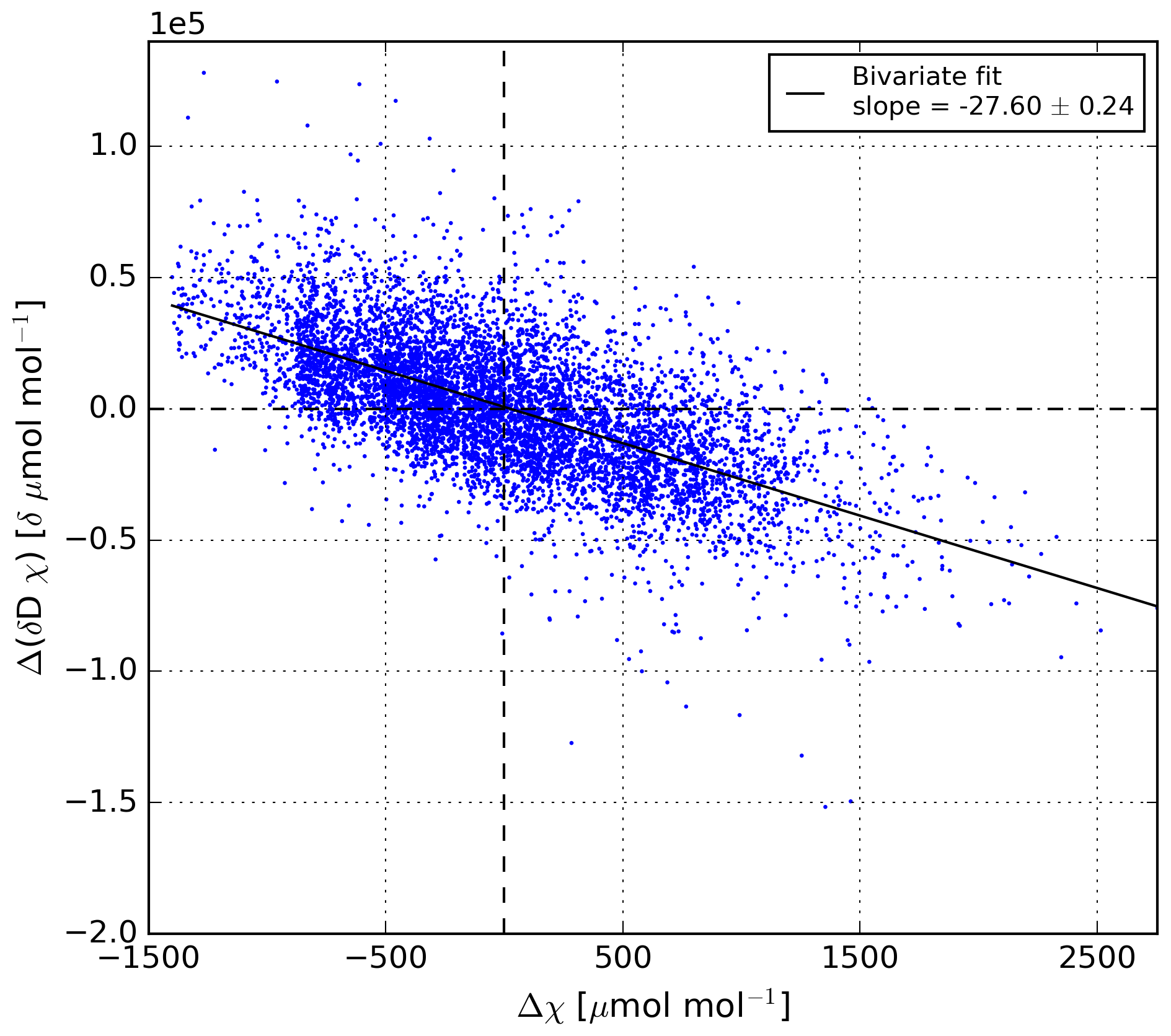
Figure A1 Example Miller-Tans analysis of the 30 min interval starting at 15:00 on 15 August 2022. The variations in δ values and H₂O mole fractions (χ) were measured using the H₂O isotope analyser measuring from the inlet at 57 m. The Δ refers to the difference between the measured value and the atmospheric background (Miller and Tans, 2003).

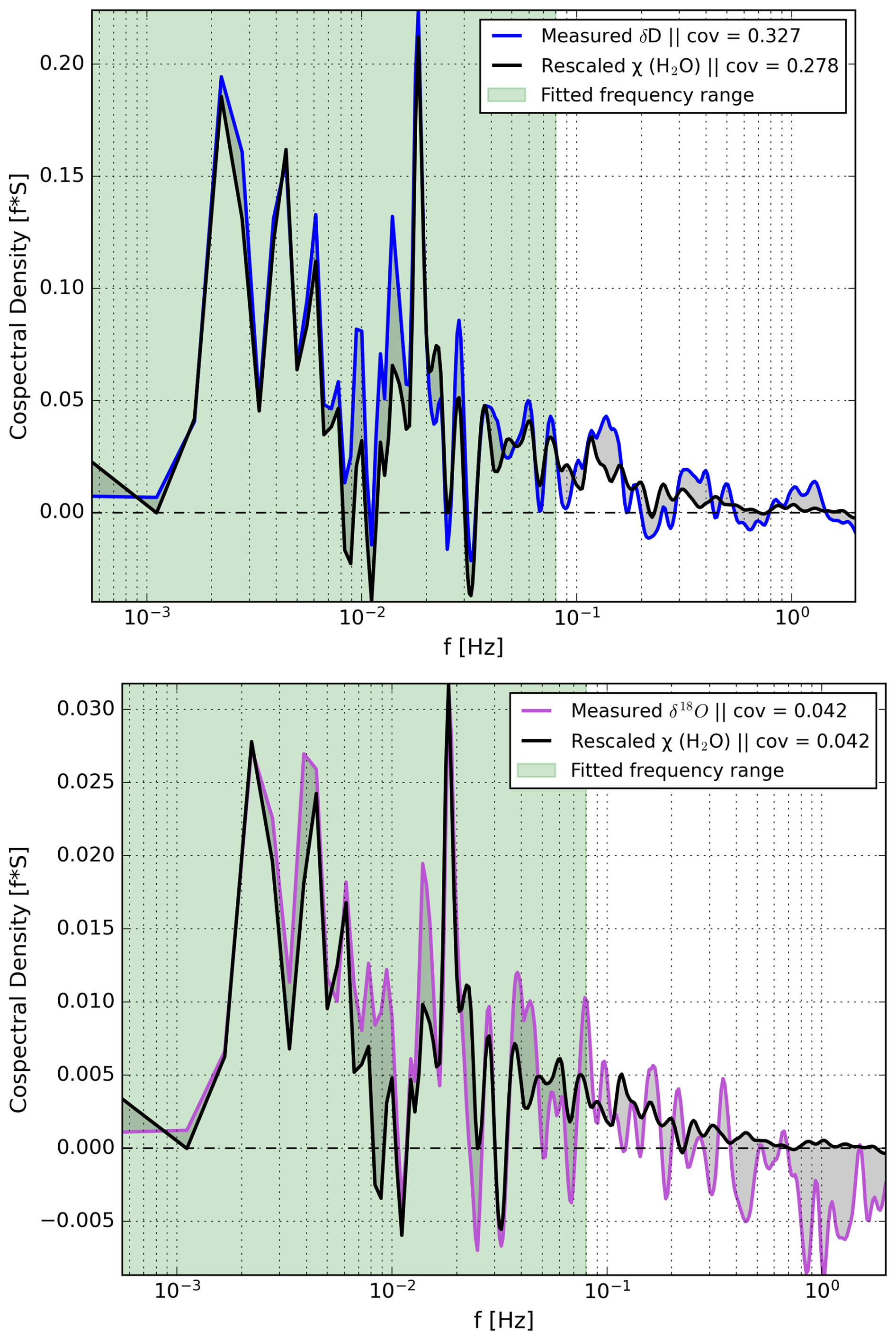
Figure A2 Example co-spectral analysis, and implementation of the spectral correction method described in Moonen et al. (2023), of the 30 min interval starting at 14:00 on 12 August 2022. Note that the covariance of both species with the vertical wind (w) is shown. The green window indicates the time scales which were used to rescale χ (H₂O). The contributions to the δ¹⁸O flux around 10⁰ have a negative sign, which we believe must be a measurement artifact.

Miller and Tans (2003)Horita and Wesolowski (1994)Farquhar et al. (1989a)Horita and Wesolowski (1994)

Table A1 Overview of the 14:00 H₂O isotopic state of the ecosystem from a 13 d composite, including intermediate results not shown in Fig. 6 of the main text. Related variables are grouped together. The groups follow the vertical gradient from the atmosphere to the soil water. “Type” specifies the data type, where m indicates that the variable was measured, s indicates that the variable was directly solved for, without assumptions, sa indicates that assumptions were required to solve for the variable, as described in the text.

Lee et al. (2009)Farquhar et al. (1993)Farquhar and Lloyd (1993)Brenninkmeijer et al. (1983)Lee et al. (2009)Lee et al. (2009)Brenninkmeijer et al. (1983)

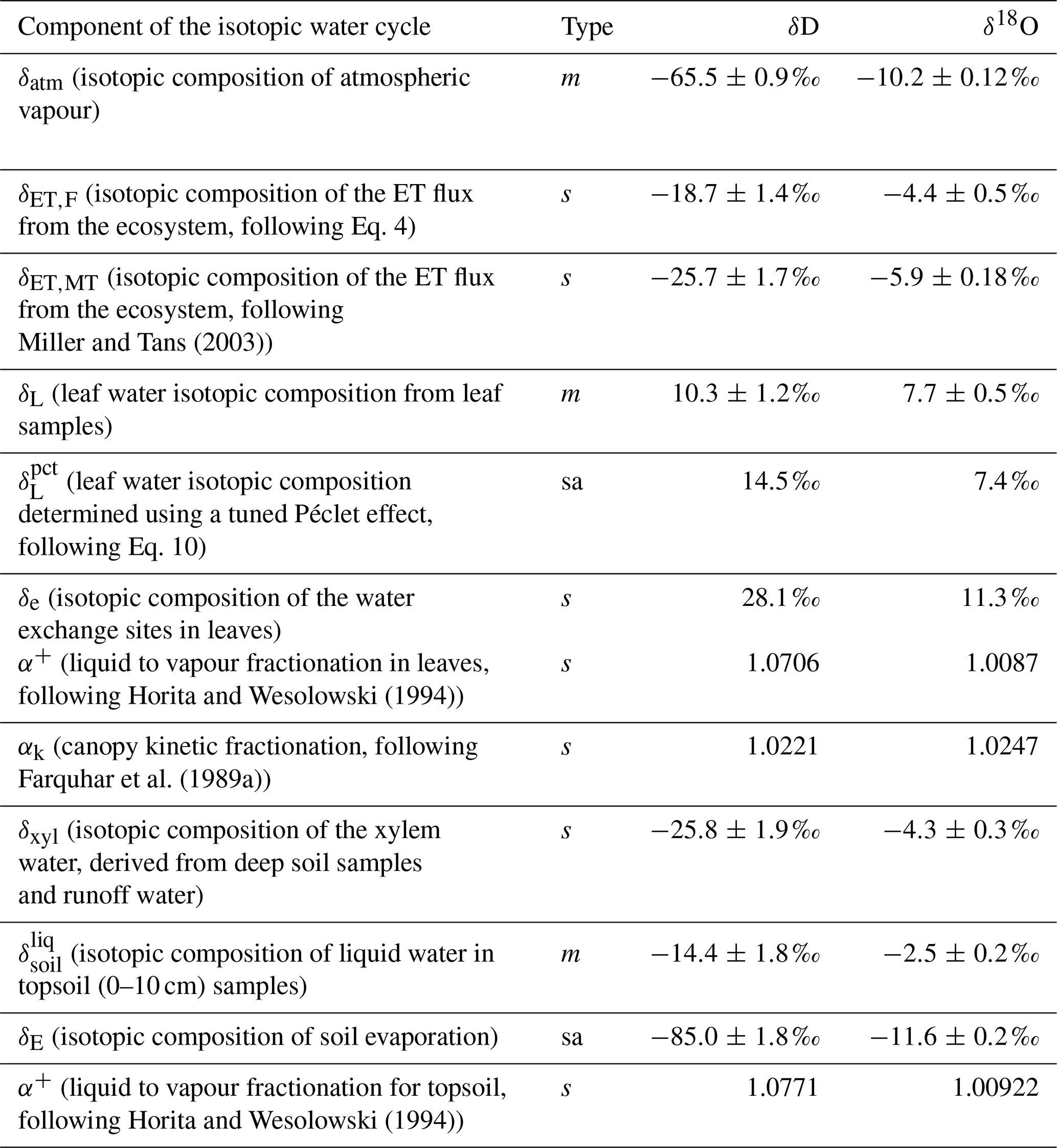
Table A2 Overview of the 14:00 CO₂ isotopic state of the ecosystem from a 13 d composite, including intermediate results. Related variables are grouped together. The groups follow the vertical gradient from the atmosphere to the soil water. “Type” specifies the data type, where m indicates that the variable was measured, s indicates that the variable was directly solved for, without assumptions, sa indicates that assumptions were required to solve for the variable.