Quantifying patterns and drivers of larval dispersal in Japanese anchovy (Engraulis japonicus) in the China Seas

Larval dispersal is a fundamental process linking marine populations and shaping individual fitness and population connectivity, making its quantification essential for understanding recruitment dynamics in fisheries. However, larval dispersal of the commercially and ecologically important Japanese anchovy (Engraulis japonicus), one of the most abundant pelagic fishes in the China Seas, remains poorly understood. Here, we applied 1D and 2D dispersal kernels to quantify larval dispersal outputs from previously published Lagrangian particle-tracking simulations, in which particles were released from seven spawning grounds across the China Seas during April–August (1987–2004) and tracked for 30–60 d. We evaluated the relative influences of spawning ground, spawning month and year, and larval travel duration, on dispersal patterns and connectivity. Larval settlement was concentrated in the Bohai Sea, the northern Yellow Sea and along the southern coast of the Shandong Peninsula, with peak densities near 39° N, identifying these regions as major nursery areas. A Weibull 1D dispersal kernel best described larval dispersal-distance distribution, with modal dispersal distances from 42.67 to 153.23 km among spawning grounds. Of the factors examined, spawning ground was the dominant driver of dispersal and connectivity, explaining 31 % of the variance. Larvae from Changjiang Estuary spawning ground dispersed more broadly to the Yellow Sea, Sea of Japan and the northwestern Pacific, whereas larvae from other grounds were largely retained within the China Seas, suggesting the Changjiang Estuary may provide a potential pathway for connectivity among regional populations. Dispersal patterns exhibited strong seasonal shifts, with enhanced eastward and northward export in spring–early summer and increased retention in late summer. Increasing larval travel duration promoted directional long-range transport while reducing occupied area, local retention and self-recruitment, indicating that longer dispersal does not imply broader spatial occupation. Pelagic larval duration captured mean dispersal trends but was a poor predictor of individual dispersal outcomes. Overall, these findings provide a quantitative framework for understanding larval dispersal dynamics and may help inform fisheries management of Japanese anchovy.

1 Introduction

Understanding and quantifying the patterns and causes of marine larval dispersal is essential for predicting population dynamics and managing marine populations, and has long been a central goal in ecology and conservation biology (Botsford et al., 2001; D'Aloia et al., 2015; Sato et al., 2023). Larval dispersal refers to the process by which larvae are transported by currents away from their source populations. Because most marine species experience a pelagic larval phase, larvae may be widely dispersed before recruiting to adult habitats, thereby linking spatially separated populations (Cowen and Sponaugle, 2009; Wood et al., 2013; Faillettaz et al., 2018; Sato et al., 2023). Direct observation of larval dispersal remains challenging due to the small size of eggs and larvae, their potential for long-distance transport, the broad spatial extent of spawning grounds, and a prolonged spawning season (Zhang et al., 2020b; Wei et al., 2003). To overcome these limitations, biophysical models (a hydrodynamic model coupled to a Lagrangian particle tracking model) have been widely applied to investigate larval dispersal in marine fishes (Paris and Cowen, 2004; Zhao et al., 2009; Lett et al., 2010; Chaput et al., 2022).

Despite the applications of these models to Japanese anchovy (Engraulis japonicus) (Itoh et al., 2009; Tu et al., 2012; Takeshige et al., 2015; Xing et al., 2020; Xing et al., 2021), however, a comprehensive and quantitative understanding of larval dispersal patterns and their underlying drivers across the China Seas remains lacking. As one of the most abundant pelagic fishes in this region, Japanese anchovy plays a key trophic role and supports both ecological functioning and fisheries production (Zhao et al., 2003). However, its biomass declined sharply from approximately three million tons prior to the mid-1990s to less than 0.5 million tons in the early 2000s, presenting major challenges for fisheries management (Zhao et al., 2003). This collapse has stimulated growing interest in the mechanisms underlying population fluctuations and recruitment dynamics, particularly the role of larval dispersal during early life stages (Tu et al., 2012; Takeshige et al., 2015; Xing et al., 2020; Liu et al., 2020). While quantifying larval dispersal patterns and their drivers, including spawning location, spawning timing (month and year), and transport duration, can provide critical insights into population connectivity and recruitment processes. Specifically, Xing et al. (2020, 2021) have applied biophysical models to investigate larval transport of Japanese anchovy, focusing on retention dynamics, larval retention areas (LRAs), and environmental influences on recruitment. However, quantitative analyses of larval dispersal patterns and drivers across China Seas remain lacking.

Dispersal kernel, the probability density function of the dispersal distance from the release location, has been long recognized as a useful framework for quantifying dispersal patterns (Cowen and Sponaugle, 2009; Ayata et al., 2010; Shi et al., 2019; Nathan, 2008; Almany et al., 2017). Because pelagic species often lack clearly defined settlement boundaries, dispersal kernels encompass both successful and unsuccessful dispersal events, avoiding arbitrary definitions of transport success (Huret et al., 2010). However, classical dispersal kernels describe dispersal as a function of distance only and do not capture directionality. These are therefore referred to as a one-dimensional (1D) dispersal distance kernels (Siegel et al., 2003). To address this limitation Edwards et al. (2007) extended the framework to two-dimensional (2D) dispersal location kernels, enabling the quantification of anisotropic dispersal patterns. Huret et al. (2010) further refined this approach by introducing spatial indices describing occupation, aggregation and dispersion.

Here, we applied both 1D and 2D dispersal kernels to quantify larval dispersal patterns of Japanese anchovy in the China Seas, using particle-tracking outputs from Xing et al. (2020) and Xing et al. (2021). We further performed a multi-factor, multi-variable analysis of variance (MANOVA) to evaluate the impacts of spawning ground, travel duration, spawning year and spawning month on dispersal, and examine the resulting implications for recruitment dynamics and stock connectivity.

2 Materials and Methods

2.1 Study Species and Study Area

In early spring, adult anchovies migrate from their offshore overwintering grounds to coastal waters to spawn (Fig. 1). Spawning occurs from April to October and peaks between May and June (Hao et al., 2003; Zhang et al., 2020b). Embryonic development requires approximately 42–72 h. Previous studies indicate that anchovy larvae begin to exhibit weak active swimming ability at a body length of 5–7 mm, with swimming capacity gradually increasing between 10 and 20 mm, and reaching a more developed stage at 20–25 mm (Masuda, 2011). Given that the present study focuses on larvae ≤ 20 mm in length (approximately within 30 d post-hatching), active swimming behaviour was neglected following previous approaches, and larvae were treated as passive particles (Takeshige et al., 2015; Xing et al., 2020).

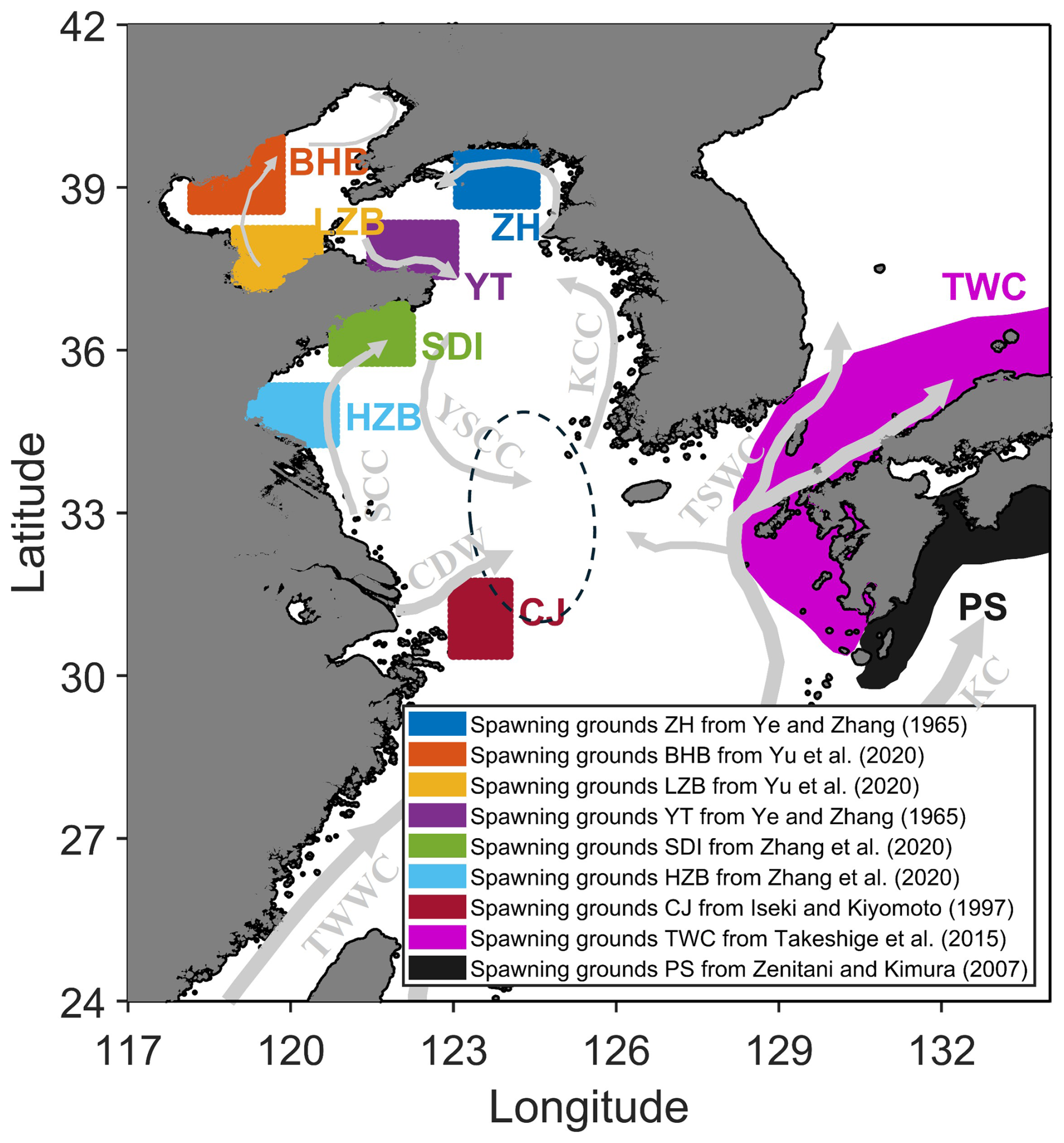
Figure 1 The spawning grounds of Japanese anchovy (Engraulis japonicus) in the China Sea, Japan Sea and Pacific Ocean, which also represent the larval particle release locations used in the particle tracking models (with the exception of TWC and PS). The areas are: Zhuanghe Bay (ZH; Ye and Zhang, 1965); northeast of Bohai Bay and Laizhou Bay (BHB and LZB, respectively; Yu et al., 2020); Yantai (YT; Ye and Zhang, 1965); south of the Shandong Peninsula and in Haizhou Bay (SDI and HZB, respectively; Zhang et al., 2020b); the Changjiang Estuary (CJ; Iseki and Kiyomoto, 1997); northwest of Kyushu (TWC; Takeshige et al., 2015); and south of Kyushu (PS; Zenitani and Kimura, 2007). The white area represents the ocean and grey represents land. The dashed ellipse represents the overwintering ground (Zhao, 2006). Grey arrows delineate major currents in summer, including the Kuroshio Current (KC), Taiwan Warm Current (TWWC), Tsushima Warm Current (TSWC), Korea Coastal Current (KCC), Yellow Sea Coastal Current (YSCC), Subei Coastal Current (SCC), and Changjiang Diluted Water (CDW).

Seven Japanese anchovy spawning grounds (located in the Bohai, Yellow, and East China Seas) were selected for this study (Fig. 1), including: Zhuanghe Bay (ZH; Ye and Zhang, 1965); northeast of Bohai Bay and in Laizhou Bay (BHB and LZB, respectively; Yu et al., 2020); Yantai (YT; Ye and Zhang, 1965); south of the Shandong Peninsula and in Haizhou Bay (SDI and HZB, respectively; Zhang et al., 2020b); and the Changjiang Estuary (CJ; Iseki and Kiyomoto, 1997). Lagrangian particles were released and tracked from these sites. Additionally, two spawning grounds for Japanese stocks were included to study connectivity: northwest of Kyushu (TWC; Takeshige et al., 2015) and south of Kyushu (PS; Zenitani and Kimura, 2007). Notably, no particles were released from these two sites.

2.2 Hydrodynamic and Lagrangian Particle Tracking Model

Lagrangian particle tracking simulation outputs from Xing et al. (2020) and Xing et al. (2021), which investigated larval retention of Japanese anchovy during 1987–2004, respectively, were applied in this study. In those simulations, passive particles representing larvae were released in surface waters throughout the Yellow Sea (YS) and the Bohai Sea (BS). From these datasets, we extracted and analyzed the trajectories of particles released from the larval release locations defined in the present study. The hydrodynamic model and Lagrangian particle tracking model were described as follows.

The particle trajectories analyzed here were taken from Xing et al. (2021) for 1987–2004. Details of the corresponding hydrodynamic-model configurations and validation are provided in those studies. Briefly, the Finite Volume Coastal Ocean Model (FVCOM) was used to simulate the hydrodynamic fields for larval dispersal. This model has been successfully applied to study larval retention of Japanese anchovy in the YS (Xing et al., 2020, 2021). The model configuration features a horizontal resolution of 6.5 km (41 sigma layers vertically), with a mesh of 44 682 nodes and 86 107 grids. The time step was 40 s and hourly current data from the published simulations were used to drive the particle tracking model. Over 4 months in 2012 and 2013 the model reproduced subtidal current velocities with root-mean-square errors of 0.70 to 3.24 cm s⁻¹.

Given the weak swimming ability of Japanese anchovy below 20 mm in length, a 2D Lagrangian particle tracking model was developed to simulate the passive transport of fish larvae, with active swimming behavior neglected (Takeshige et al., 2015; Xing et al., 2020). In this algorithm, a fourth-order Runge-Kutta scheme was used to prevent excessively large truncation errors. Random walk was also considered to resolve sub-grid scale phenomenon, such as horizontal turbulent flow (Willis, 2011; Choi et al., 2018). The horizontal diffusivity coefficient was based on the Smagorinsky diffusivity scheme (Choi et al., 2018). The time step for this particle tracking model was set as 1 h. The hydrodynamic fields from the FVCOM simulation served as the driver for the particle movements. A comprehensive description of the algorithm is provided by Xing et al. (2020). Larval release was specified as follows.

• Larval release location. Larval particles were released from the seven spawning grounds identified in China Seas in Fig. 1 (ZH, BHB, LZB, YT, SDI, HZB, CJ). Each site was divided into ∼ 150 grid cells, consistent with the FVCOM grid. All particles were released from the center of the grid; and they were released in the surface layer (the uppermost sigma layer of FVCOM model) as living eggs and larvae for Japanese Anchovy have typically been found near the surface (Iseki and Kiyomoto, 1997). Larval vertical migration and larval mortality were not considered in this study. To minimize the influence of release-area size, we used standardized rectangular release areas for each release location.

• Larval release time. To study the effects of spawning month and year on larval dispersal, particles were released annually on the 1st, 11th, and 21st of each month from April to August during 1987–2004 (Xing et al., 2021). This resulted in 15 releases per year (3 times per month × 5 months), totalling 270 release events over the 18-year period (15 times per year × 18 years).

• Larval tracking duration. The pelagic larval duration (PLD) ranges from 30 to 60 d (Takeshige et al., 2015; Huggett et al., 2003; Lett et al., 2006; Xing et al., 2020; Xing et al., 2021; Lett et al., 2007). Accordingly, larval tracking was conducted with durations of 30, 40, 50, 60 d, respectively.

• Larval release number. A total of 1134000 particles (7 spawning grounds × 150 grid cells per site × 18 years × 15 times per year × 4 durations = 1 134 000 particles) were released in this simulation.

• Larval settlement location. The position of a particle stopped at the end of its PLD is referred to as its settlement location.

2.3 1D Dispersal Distance Kernel

The 1D dispersal kernel has been long recognized as a useful approach to quantify dispersal patterns of plant seeds, insects and fish larvae (Cowen and Sponaugle, 2009; Ayata et al., 2010; D'Aloia et al., 2015; Almany et al., 2017; Shi et al., 2019; Shi et al., 2024). It represents the probability density function (PDF) of these dispersal distances, which is defined as the straight-line distance between a particle release location and its settlement location. In this study, dispersal distances from all 18 simulated years were aggregated for each spawning ground to compute a unique kernel for each ground. Additionally, a separate, combined kernel was calculated by pooling dispersal distances from all grounds, resulting in a total of eight dispersal kernels (seven for the individual grounds and one collective kernel).

The kernel can provide three important metrics characterizing larval dispersal: local retention, mean- (or median-) dispersal distance, and long-distance dispersal (Nickols et al., 2015). Local retention is the ratio of locally produced settlement to total local larval release, determining the self-persistence of a population (Botsford et al., 2009). The median-dispersal distance describes the distance within which half of larvae settle. Long-distance dispersal, usually defined as the 95th-percentile dispersal distance, is important for estimating population invasion, population spread, and genetic connectivity (Cowen and Sponaugle, 2009; Nathan, 2008; Nathan et al., 2008). Self-recruitment, which is related to but distinct from local retention (Botsford et al., 2009), was also computed. It represents the ratio of locally produced settlement to settlement from all origins at a site.

2.4 2D Dispersal Location Kernel

The kernel above is a function of distance only, and does not convey information on direction. It is thus referred to as a “one-dimensional (1D) dispersal distance kernel” (Siegel et al., 2003). Edwards et al. (2007) extended the 1D kernel into two dimensions (2D), as a “2D dispersal location kernel”, by computing a set of indices to describe the kernel in areas with strong anisotropy in circulation. Huret et al. (2010) further refined this approach by introducing spatial indices related to spatial occupation and aggregation. Several indices were defined to characterize the 2D larval dispersal location kernels, enabling statistical analysis of the particle distributions (Edwards et al., 2007; Ayata et al., 2010; Hinrichsen et al., 2012; Puckett et al., 2014).

• The geographic position of the settlement locations, included the center of gravity, x_m, y_m, along with the associated variances and covariance, S_x, S_y, and S_xy.

• The mean relative transport, included the mean orthodromic distance and direction from release center (x₀, y₀) to settlement center (x_m, y_m), i.e., d_m and θ. Here, θ represents the direction measured clockwise from north.

  $$\begin{array}{}\text{(1)}& {\displaystyle }\begin{array}{rl}{d}_{\mathrm{m}}& =R_e\mathrm{acos}\left[\sin {\displaystyle \frac{\mathit{\pi }{y}_{\mathrm{m}}}{\mathrm{180}}}\sin {\displaystyle \frac{\mathit{\pi }{y}_{\mathrm{0}}}{\mathrm{180}}}+\cos {\displaystyle \frac{\mathit{\pi }{y}_{\mathrm{m}}}{\mathrm{180}}}\right.\\ & \left.\cos {\displaystyle \frac{\mathit{\pi }{y}_{\mathrm{0}}}{\mathrm{180}}}\cos \left({\displaystyle \frac{\mathit{\pi }{x}_{\mathrm{0}}}{\mathrm{180}}}-{\displaystyle \frac{\mathit{\pi }{x}_{\mathrm{m}}}{\mathrm{180}}}\right)\right]\end{array}\text{(2)}& {\displaystyle }\begin{array}{rl}\mathit{\theta }& =\arctan \mathrm{2}\left(\sin \left({\displaystyle \frac{\mathit{\pi }{x}_{\mathrm{m}}}{\mathrm{180}}}-{\displaystyle \frac{\mathit{\pi }{x}_{\mathrm{0}}}{\mathrm{180}}}\right)\cos \left({\displaystyle \frac{\mathit{\pi }{y}_{\mathrm{m}}}{\mathrm{180}}}\right),\right.\\ & \cos \left({\displaystyle \frac{\mathit{\pi }{y}_{\mathrm{0}}}{\mathrm{180}}}\right)\sin \left({\displaystyle \frac{\mathit{\pi }{y}_{\mathrm{m}}}{\mathrm{180}}}\right)-\sin \left({\displaystyle \frac{\mathit{\pi }{y}_{\mathrm{0}}}{\mathrm{180}}}\right)\\ & \left.\cos \left({\displaystyle \frac{\mathit{\pi }{y}_{\mathrm{m}}}{\mathrm{180}}}\right)\cos \left({\displaystyle \frac{\mathit{\pi }{x}_{\mathrm{m}}}{\mathrm{180}}}-{\displaystyle \frac{\mathit{\pi }{x}_{\mathrm{0}}}{\mathrm{180}}}\right)\right)\times {\displaystyle \frac{\mathrm{180}}{\mathit{\pi }}}\end{array}\end{array}$$

• The dispersion or variance around the center of gravity is the inertia (I). It is the mean square distance between an individual fish and the center of gravity of the population (Woillez et al., 2009). It is not identical in every spatial direction, and can be decomposed into two principal orthogonal axes, which represent the maximum (amaj) and the minimum (amin) components overall inertia. A principal component analysis (PCA) of particle positions provides these axes, which can be visualized in space as an ellipse. The ellipse characteristics include the length of the major axis (amaj), its orientation (θ_m), the length of the minor axis (amin), and the isotropy (iso).

  $$\begin{array}{}\text{(3)}& {\displaystyle }I={\displaystyle \frac{\mathrm{1}}{n}}\sum _{i=\mathrm{1}}^n\left(\right(x_i-x_{\mathrm{m}}{)}^{\mathrm{2}}+(y_i-y_{\mathrm{m}}{)}^{\mathrm{2}})\text{(4)}& {\displaystyle }\mathrm{amaj}=\sqrt{{\displaystyle \frac{\mathrm{1}}{\mathrm{2}}}\left(S_x+S_y+\sqrt{{\left(S_x-S_y\right)}^{\mathrm{2}}+\mathrm{4}{S}_{xy}^{\mathrm{2}}}\right)}\text{(5)}& {\displaystyle }\mathrm{amin}=\sqrt{{\displaystyle \frac{\mathrm{1}}{\mathrm{2}}}\left(S_x+S_y-\sqrt{{\left(S_x-S_y\right)}^{\mathrm{2}}+\mathrm{4}{S}_{xy}^{\mathrm{2}}}\right)}\text{(6)}& {\displaystyle }{\mathit{\theta }}_{\mathrm{m}}={\displaystyle \frac{\mathrm{180}}{\mathit{\pi }}}\cdot {\displaystyle \frac{\mathrm{1}}{\mathrm{2}}}\arctan \mathrm{2}(\mathrm{2}{S}_{xy},S_x-S_y)\text{(7)}& {\displaystyle }\mathrm{iso}={\displaystyle \frac{\mathrm{amin}}{\mathrm{amaj}}}\end{array}$$

• For a given inertia, the spatial distribution of particles can exhibit a range of patterns at smaller scales, depending on how space is occupied, from a homogeneous density distribution to pronounced aggregations. To characterize these spatial patterns, we used indices developed by Woillez et al. (2009) for analyzing adult fish populations: positive area (PA), spreading area (SA), equivalent area (EA), and the coefficient of variation of positive values of densities (CV₀). PA is defined as the sum of area units containing at least one particle, calculated as the number of grids with at least on particle multiplied by the area of each grid (S). SA quantifies how densities are distributed within the PA, as follows:

  $$\begin{array}{}\text{(8)}& \mathrm{SA}=\mathrm{2}\int {\displaystyle \frac{\left(Q-Q\left(A\right)\right)}{Q}}\mathrm{d}A\end{array}$$

  where A is the cumulated area occupied by the density values, ranked in decreasing order. Q(A) is the corresponding cumulated abundance and Q is the total abundance. EA measures the inverse probability that two randomly chosen particles settled in the same grid cell. It is defined as:

  $$\begin{array}{}\text{(9)}& \mathrm{EA}={\displaystyle \frac{S\times ({\sum }_i{d}_i{)}^{\mathrm{2}}}{{\sum }_i{d}_i^{\mathrm{2}}}}\end{array}$$

  where d_i is the particle density in cell i of the model domain. Finally, CV₀ is defined as:

  $$\begin{array}{}\text{(10)}& {\mathrm{CV}}_{\mathrm{0}}^{\mathrm{2}}={\displaystyle \frac{\mathrm{PA}}{\mathrm{EA}}}-\mathrm{1}\end{array}$$

2.5 Statistical Analysis

We performed a multi-factor, multi-variable analysis of variance (MANOVA) to evaluate the impacts of spawning ground, travel duration, spawning year and spawning month on dispersal. Variables comprised seven metrics: (i) the geographic position of the center of gravity (x_m, y_m, S_x, S_y, and S_xy), (ii) the mean relative transport indices (mean distance and direction of the center of gravity from the release location, d_m and θ), (iii) the ellipse characteristics (I, amaj, amin, iso, and θ_m), (iv) spatial and aggregation indices (PA, SA, EA and CV₀), (v) connectivity between each spawning ground (${\sum }_i{C}_{i,\mathrm{ZH}}$, ${\sum }_i{C}_{i,\mathrm{BHB}}$, ${\sum }_i{C}_{i,\mathrm{LZB}}$, ${\sum }_i{C}_{i,\mathrm{YT}}$, ${\sum }_i{C}_{i,\mathrm{SDI}}$, ${\sum }_i{C}_{i,\mathrm{HZB}}$, ${\sum }_i{C}_{i,\mathrm{CJ}}$, ${\sum }_i{C}_{i,\mathrm{TWC}}$, ${\sum }_i{C}_{i,\mathrm{PS}}$), (vi) local retention, and (vii) self-recruitment. The MANOVA was performed using the 50-50 MANOVA Matlab^® code from Langsrud (2002), which is designed to handle multiple highly collinear response variables.

3 Results

3.1 Dispersal Patterns

Japanese anchovy larvae were simulated to settle over a wide range, while were concentrated in the BS, the northern YS and along the southern coast of the Shandong Peninsula, with peak densities near 39° N, identifying these regions as major nursery grounds. From 1987–2004, larvae dispersed widely during their pelagic stage, encompassing the Bohai, Yellow, and East China seas, the Korea Strait, the Sea of Japan, and the northwestern Pacific (Fig. 2). Settlement density gradually decreased southward and offshore (except in the BS), consistent with a predominantly northward transport pattern driven by regional circulation (Xing et al., 2020).

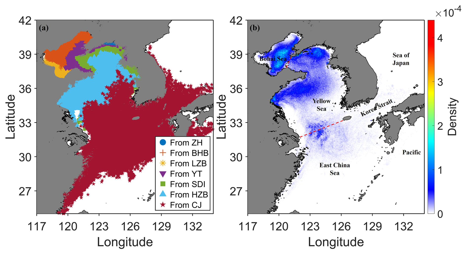
Figure 2 (a) Larval settlement patterns of Japanese anchovy (Engraulis japonicus) for different spawning grounds, integrated across all spawning months, spawning years, and tracking durations. White areas represent the ocean, grey areas represent land, and each color corresponds to settlement locations originating from a specific spawning ground. (b) Density distribution of all settled larvae, calculated as the number of larvae settled in each cell divided by the total number of settled larvae.

We estimated the 1D dispersal kernel by fitting various PDFs to the modelled dispersal distances. The best-fitting 1D dispersal kernel was a Weibull function (Table S1 in the Supplement; Fig. 3):

$$\begin{array}{}\text{(11)}& \mathit{\rho }\left(d\right)={\displaystyle \frac{a}{\mathit{\lambda }}}({\displaystyle \frac{d}{\mathit{\lambda }}}{)}^{a-\mathrm{1}}\cdot e^{-(d/\mathit{\lambda }{)}^a}\end{array}$$

where ρ(d) is the probability density function, d is the dispersal distance (in kilometers). The scale parameter is λ=164.31, and the shape parameter is a=1.48. The modal dispersal distance was 73.31 km, the median-dispersal distance was 128.37 km, and the long-distance dispersal threshold was 344.03 km.

3.2 Variation in Dispersal

3.2.1 Quantifying Effects on the Dispersal and Connectivity

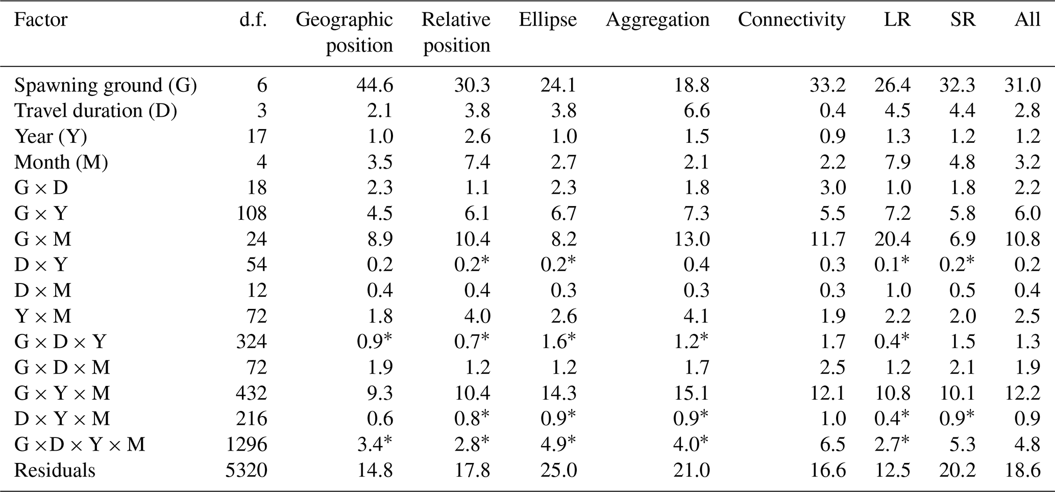
MANOVA revealed that all factors (spawning ground, travel duration, spawning year and spawning month), and most of their interactions, significantly affected the metrics (p-value were < 0.05 in most cases; Table 1), while spawning ground was the most influential, and spawning year was the least influential. Specifically, spawning ground explained the greatest amount of variance (31.0 %) in the dispersal kernel and connectivity. It also accounted for the highest proportion of variance within each set of indices: geographic position (44.6 %), connectivity (33.2 %), self-recruitment (32.3 %), relative position (30.3 %), local retention (26.4 %), ellipse (24.1 %), and aggregation (18.8 %). In contrast, spawning year explained the smallest proportion of variance across indices, including relative position (2.6 %), ellipse (1.0 %), aggregation (1.5 %), local retention (1.3 %), self-recruitment (1.2), and had the lowest overall effect on the combined indices (1.2 %). Spawning month contributed the second-highest proportion of variance for most set of indices, for instance, 3.5 % for geographic position, 7.4 % for relative position, 2.2 % for connectivity, 7.9 % for local retention, and 4.8 % for self-recruitment.

Table 1 Results of a MANOVA performed on six sets of response variables: (i) the geographic position of the center of gravity for settled particles, (ii) the relative position of the center of gravity (i.e., the distance and direction from the release locations' center of gravity to the settlement locations' center of gravity), (iii) parameters of the variance of the distribution (ellipse), (iv) parameters related to space occupation and aggregation, (v) connectivity between each spawning grounds, (vi) local retention (LR), (vii) self-recruitment (SR), and (viii) the whole set of parameters (all). Values are percentages, representing the proportion of variance in one set of response variable that is explained by each factor. An asterisk (^*) denotes non-significant effects (p> 0.05).

3.2.2 Spatial Variability of Dispersal

Since the spawning ground contributed most to the variance in larval dispersal, the spatial variability of the dispersal patterns was presented (Figs. 2a and S1), 1D and 2D dispersal kernels were computed (Figs. 3a, b and 4).

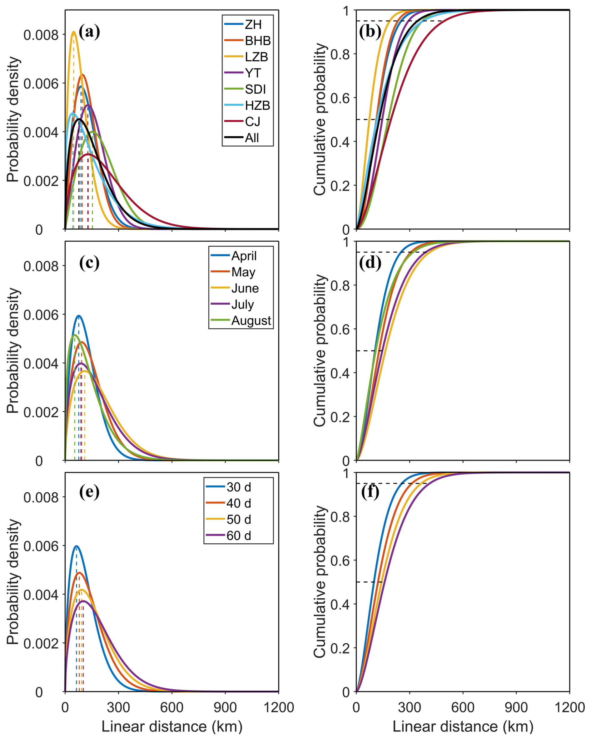
Figure 3 Dispersal kernel, the probability density function (PDF) of dispersal distances between spawning grounds and settlement locations, for Japanese anchovy (Engraulis japonicus) larvae, by (a) spawning ground, (c) spawning month, and (e) travel duration. (b) Cumulative distribution function (CDF) of dispersal distances, by (b) spawning ground, (d) spawning month, and (f) travel duration. Dashed lines in the left panel represent modal dispersal distances. Dashed lines in the right panel at y=0.5 and y=0.95 represent median-dispersal distance and long-distance dispersal, respectively.

Settlement locations differed significantly between the spawning grounds: larvae from BHB and LZB (located in the BS) settled primarily within the BS; larvae from ZH, YT, SDI, and HZB (located in the YS) settled in the Yellow Sea; whereas larvae from CJ dispersed more broadly, reaching the YS, the Sea of Japan and the northwestern Pacific (Fig. S1). From 1987–2004, all Japanese anchovy larvae from ZH, BHB, LZB, and YT settled exclusively in the Bohai and YSs, with none reaching the East China Sea, Sea of Japan and Pacific (Fig. S1). Most larvae from SDI and HZB also settled in the Bohai and YSs, though a few reached the East China Sea (∼ 1.5 %–3 %) and the Jeju Strait (< 2 %). Notably, none from these northern grounds (ZH, BHB, LZB, YT, SDI, and HZB) settled in the Tsushima Strait or near Kyushu, underscoring the Bohai and YSs as key nursery areas. In contrast, larvae from CJ dispersed more widely, settling in the YS, East China Sea, Korea Strait (comprising the Jeju and Tsushima Straits), and waters off Kyushu (Fig. 2a). Many reached waters associated with Japanese nursery regions, suggesting that CJ may provide a pathway for larval exchange between regional populations. However, these simulations alone do not demonstrate effective stock connectivity. This is shown by zero-dispersal from the other more northern grounds, but relatively high dispersal from CJ to TWC and PS regions (Fig. 4).

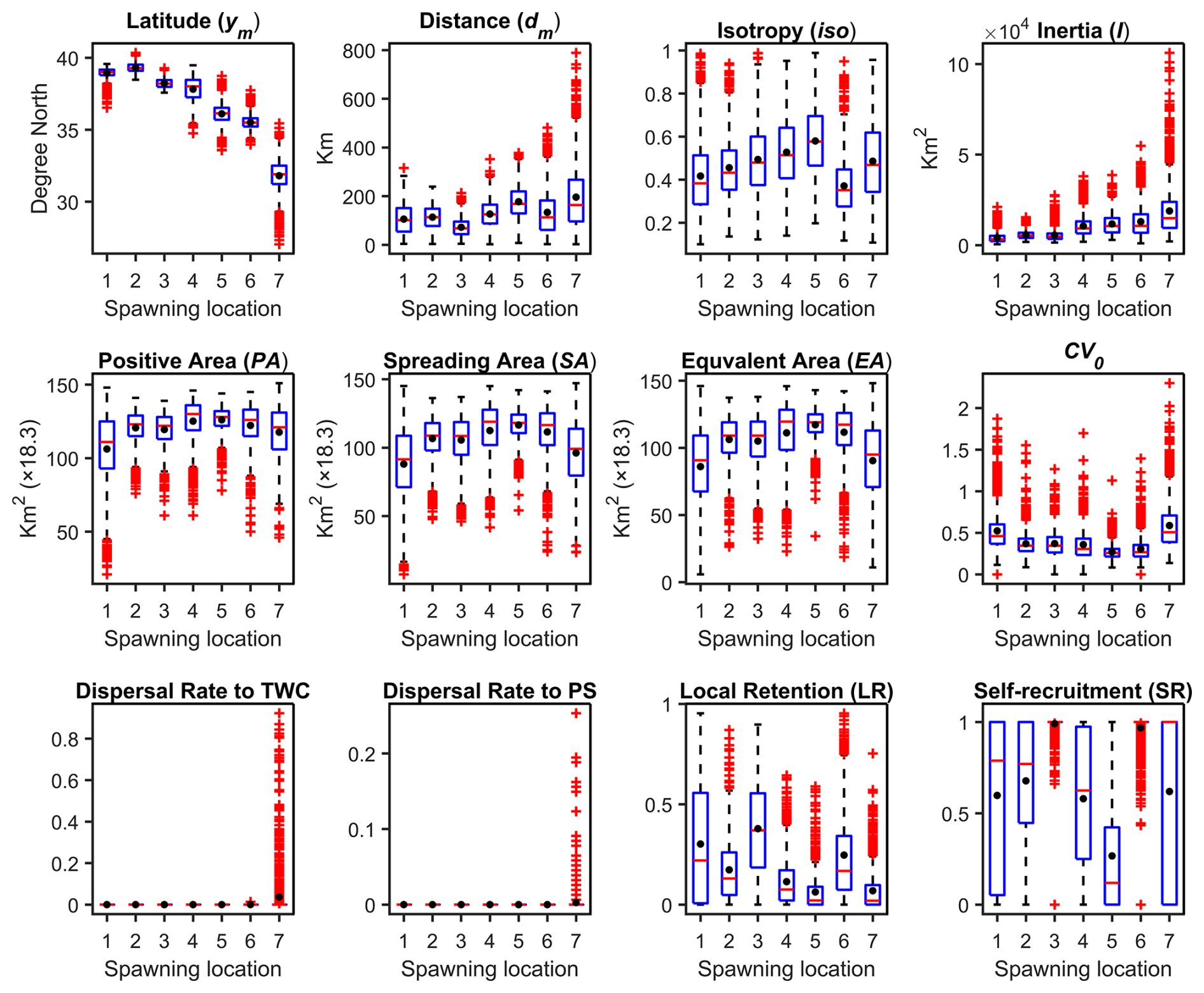
Figure 4 Box plots and means of selected indices describing the dispersal of Japanese anchovy (Engraulis japonicus) from seven discrete spawning locations. Extreme values, defined as outliers, are represented by dots. Statistics were computed from the 4 travel durations and 15 release dates per year over the periods 1987-2-004. Locations 1 to 7 correspond to the spawning locations ZH, BHB, LZB, YT, SDI, HZB, and CJ, respectively.

Dispersal kernels varied markedly among spawning grounds, with CJ exhibiting dispersal distance approximately twice those of LZB. Larvae from CJ, compared to from other grounds, exhibited the second largest modal dispersal distance (129 km), the largest median-dispersal distance (195 km) and the greatest long-distance dispersal threshold (495 km). This indicates that larvae originating from CJ settled at greater distances overall, with 50 % of individuals dispersing farther than 195 km and 5 % dispersing farther than 495 km. The CJ ground provided greater opportunities for larval transport over long distances and into the Sea of Japan and northwestern Pacific. In contrast, larvae from LZB exhibited the second smallest modal dispersal distance (48 km), the smallest median-dispersal distance (73 km), and the smallest long-distance dispersal threshold (188 km). For larvae released from ZH, BHB, LZB, YT, SDI, HZB, and CJ, the modal dispersal distances were 43 to 153 km (Fig. 3a); the median-dispersal distances were 73 to 195 km (Fig.  3b); the long-distance dispersal thresholds were 188 to 495 km, respectively (Fig. 3b). The modal dispersal distances were considered to be the most important nursery region, as the frequency of larval settlement was highest within this range. The PDF kernels became progressively flatter for LZB, BHB, ZH, YT, HZB, SDI, and CJ, with corresponding kurtosis of 8.3 to 6.1, 5.5, 4.61, 4.6, 3.4 and 2.5 (Fig. 3a).

Several sets of indices varied significantly between the spawning grounds (Fig. 4). Larvae from CJ exhibited the greatest mean orthodromic distance (d_m), the largest dispersion around their centre of gravity (Inertia), the highest spatial heterogeneity in density (CV₀), and the highest dispersal rate to the TWC and PS regions, yet one of the smallest local retention (LR) values. Notably, despite their longer dispersal, they exhibited one of the smallest PA, SA, or EA. This suggests that, although they travelled farther, their dispersal was strongly directional and spatially aggregated, resulting in lower PA, as reflected by the high spatial heterogeneity in density (CV₀). In contrast, larvae from LZB exhibited the shortest d_m, with the highest LR and SR.

3.2.3 Seasonal Variability of the Dispersal

The spawning month accounted for the second-highest proportion of variance in geographic position, relative position, and ellipse indices. The settlement location distributions (Fig. 5), 1D dispersal kernel (Fig. 3c and d) and 2D dispersal kernel metrics (Fig. 6) by spawning month were thus presented.

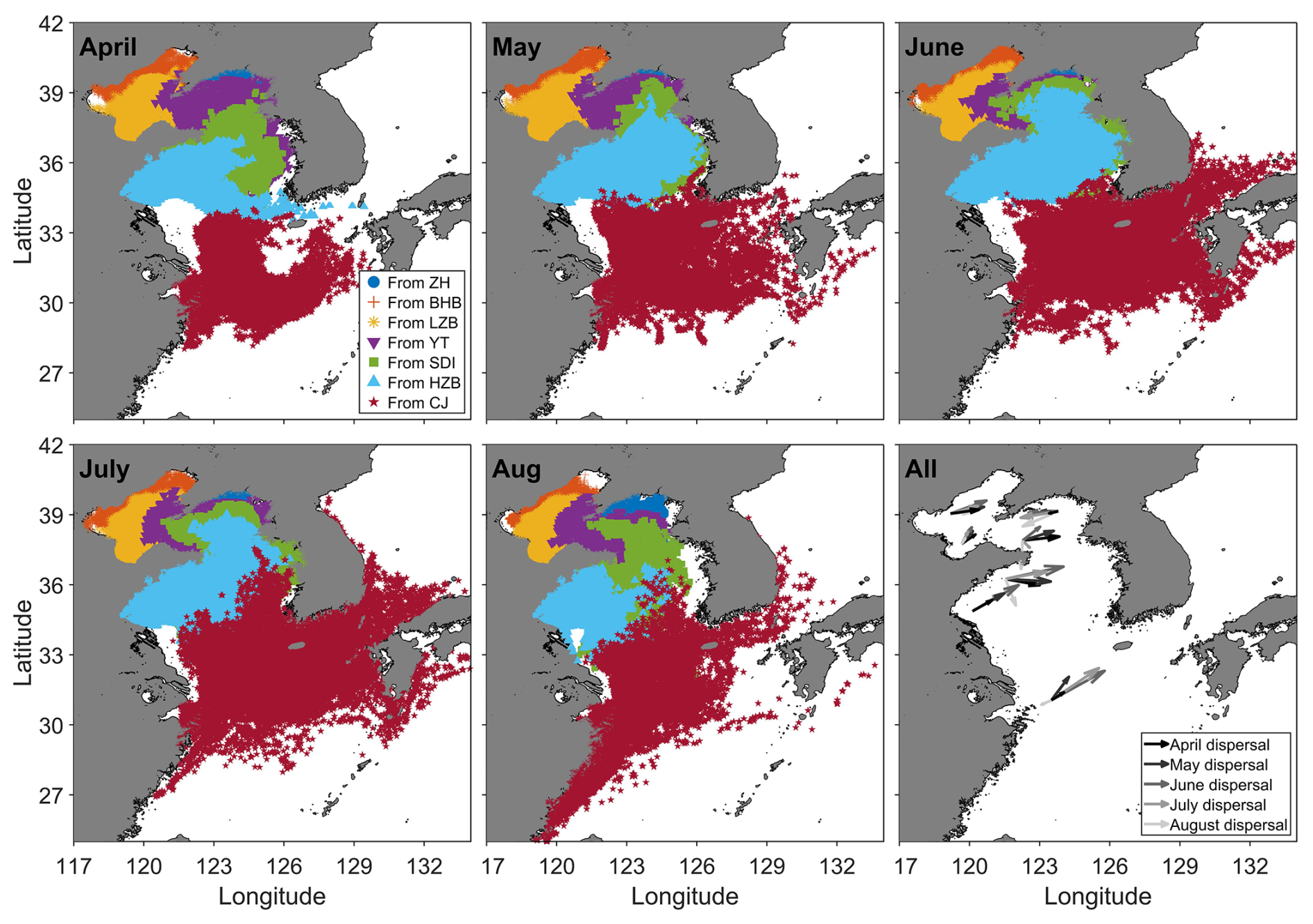
Figure 5 Larval settlement patterns of Japanese anchovy (Engraulis japonicus) by spawning ground and month. The white area represents the ocean, grey represents land, and each color corresponds to settlement locations from a specific spawning ground. Arrows in the bottom right panel indicate the mean larval dispersal from the release center to the settlement center. The arrow color turns from black to light grey as the season progresses and indicates the mean distance and direction from the center of gravity of release locations to the center of gravity of settlement locations.

A clear seasonal shift in dispersal was observed: most larvae moved eastward and northward from April to June, but shifted westward and southward since July (Fig. 5); correspondingly, local retention declined initially and increased since July (Fig. 6). The center of gravity of settlement was predominantly located east of the release locations for most groups, except for the ZH group, which exhibited a westward displacement (Fig. 5, bottom right panel). Interestingly, the settlement center of gravity shifted eastward and northward from April to June, but shifted westward and southward since July (Fig. 5, bottom right panel). The modal dispersal distance, median dispersal distance, and long-distance dispersal threshold from 1D dispersal kernel, increased from April to June and decreased from July to August (Fig. 3c and d). The d_m, I, and dispersal rate to TWC from the 2D dispersal kernel, increased from April to June and decreased from July to August, whereas LR and SR showed the opposite trend (Fig. 6).

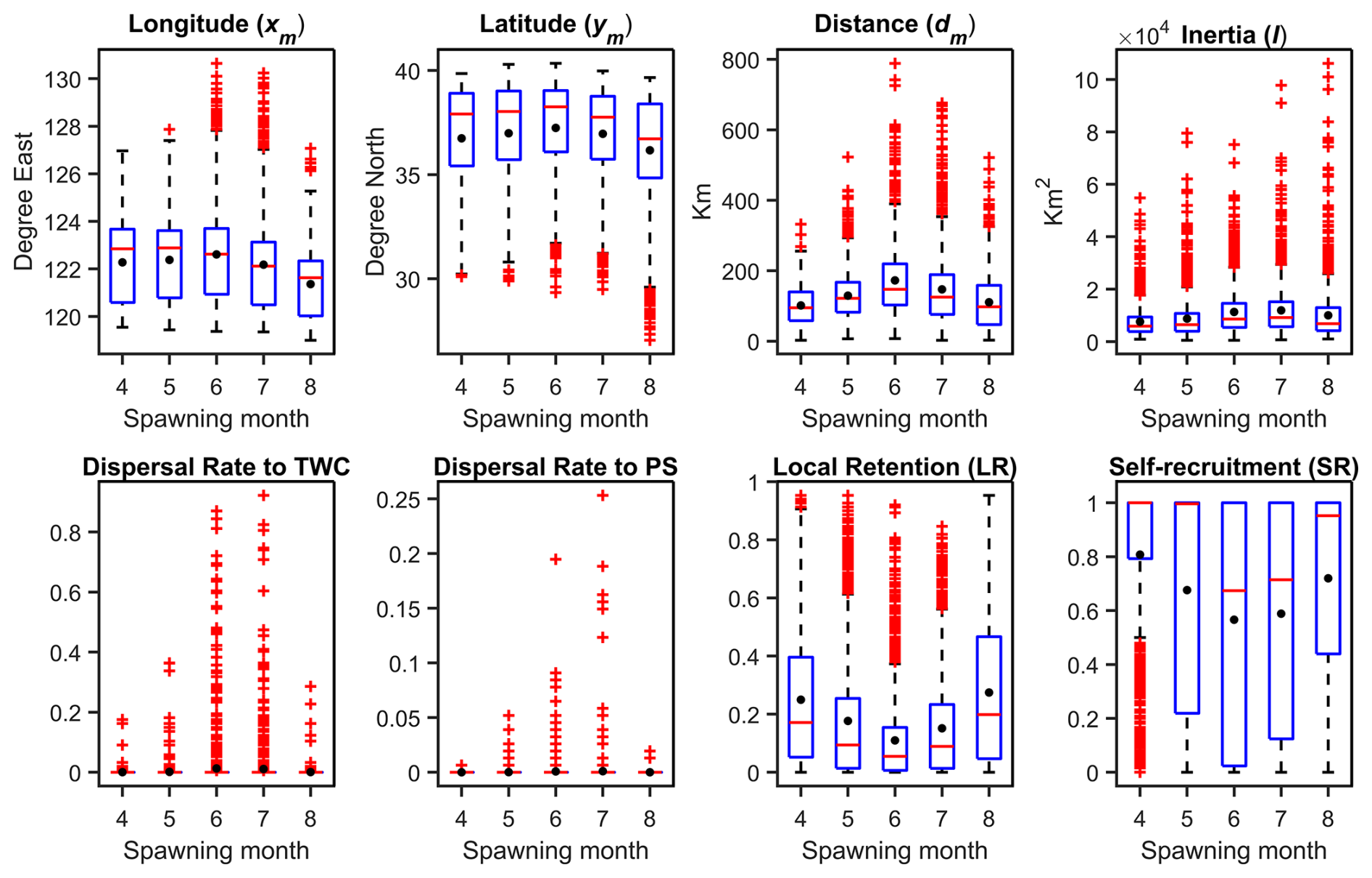
Figure 6 Box plots and means of selected indices describing the dispersal of Japanese anchovy (Engraulis japonicus) from April (month 4) through August (month 8). Extreme values, defined as outliers, are represented by red plusses. Statistics were computed from the 4 travel durations and 7 spawning locations per year over the periods 1987–2004.

3.2.4 Impact of Larval Travel Duration on Dispersal

Mean orthodromic distance from release centre to settlement centre (d_m) increased with travel duration, while PA (the sum of area units containing at least one particle) decreased, indicating that a longer dispersal distance does not necessarily correspond to a broader dispersal region. The 1D dispersal kernels (PDF) became progressively flatter from 30 to 60 d, while modal dispersal distance, median dispersal distance, and long-distance dispersal threshold all increased from 30 to 60 d (Fig. 3e and f). Several indices related to the 2D kernel varied approximately linearly with increasing travel duration (Fig. 7): the longitude of settlement centre (x_m) shifted eastward by 0.1°, d_m increased by 21.2 km, PA decreased by 3.9 × 18.3 km², inertia (I) increased by 2055 km², local retention (LR) decreased by 0.04 and self-recruitment (SR) decreased by 0.07, per 10 d.

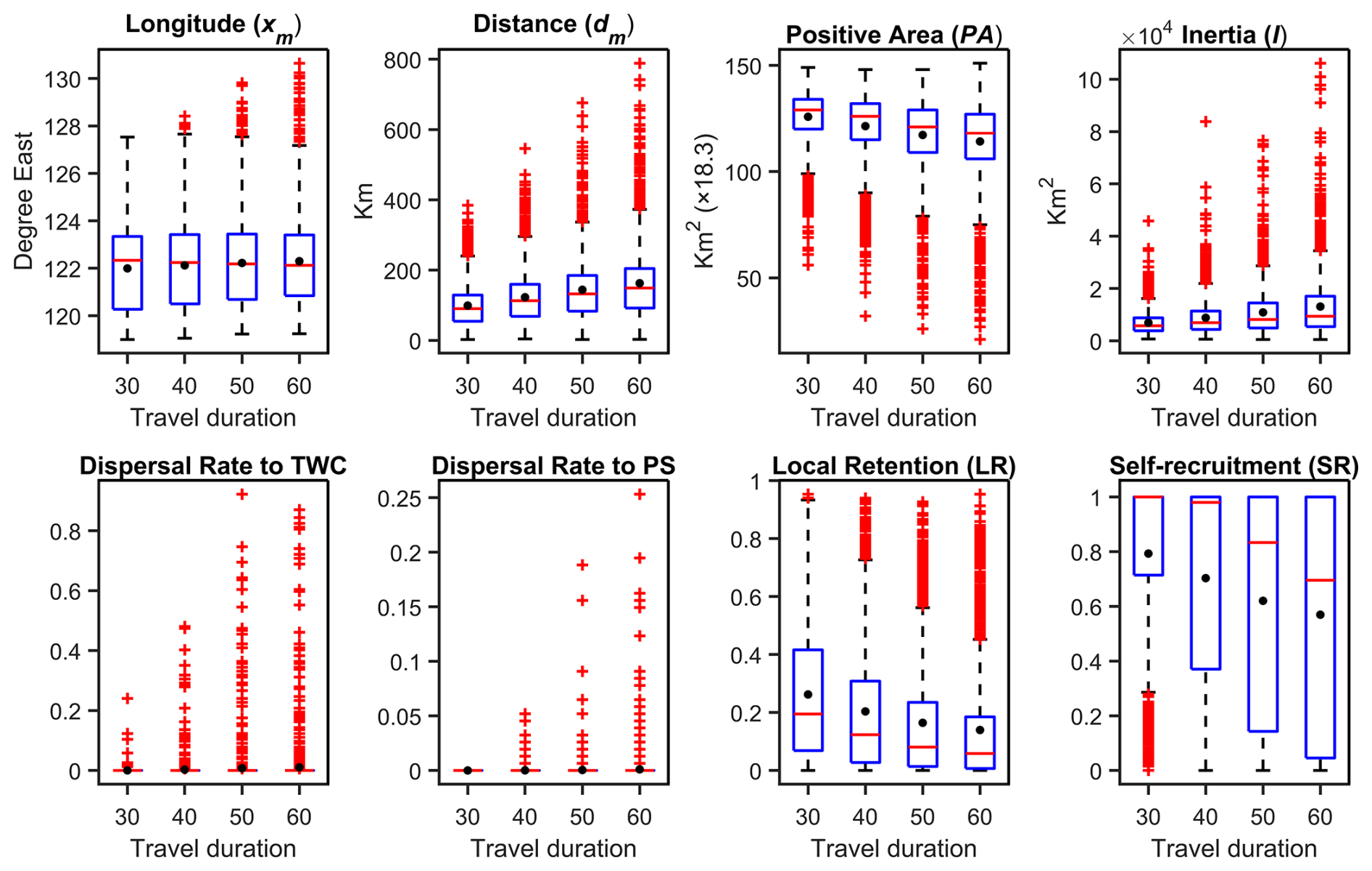
Figure 7 Box plots and means of selected indices describing the dispersal of Japanese anchovy (Engraulis japonicus) in 4 travel durations. Extreme values, defined as outliers, are represented by dots. Statistics were computed from the 7 spawning locations and 15 release dates per year over the periods 1987–2004.

3.2.5 Interannual Variability of Dispersal

Spawning year explained the smallest proportion of variance in geographic position, relative position, ellipse metrics, aggregation, and the LR and SR indices (Table 1). Interannual variability in larval dispersal patterns is illustrated in Fig. S2 and further quantified using the latitude of the settlement center (Fig. 8). For all spawning grounds, the settlement center exhibited a slight southward shift over time, as indicated by the negative slopes of the fitted regression lines. However, these trends were weak, as reflected by the low R² values.

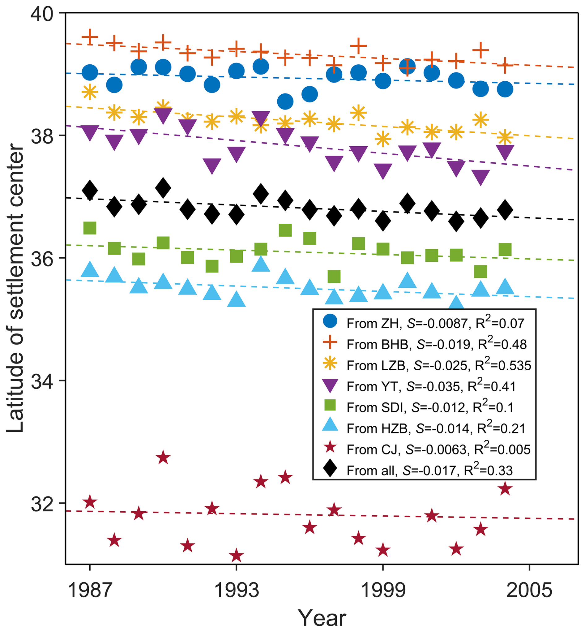
Figure 8 Interannual variability in the latitude of the settlement center of Japanese anchovy (Engraulis japonicus) larvae. S represents the slope of the fitted line.

4 Discussion

4.1 Larval Dispersal Patterns of Japanese Anchovy

The modeled larval dispersal patterns in the present study are generally consistent with the observations reported by Wan et al. (2002), partly consistent with those of Wan et al. (2008), and partly inconsistent with the patterns described by Zhang et al. (2025). In Wan et al. (2002), larval abundance decreased along a survey transect extending from approximately 120.6° E, 35.9° N to 125.8° E, 33.0° N, consistent with the density gradient shown in Fig. 2b. Furthermore, along the transect from 123.0° E, 31.0° N to 125.8° E, 33.0° N, larval abundance peaked near the midpoint of the transect (approximately 125.0° E, 32.5° N), corresponding closely to the high-density region simulated in the northern East China Sea (Fig. 2b). Wan et al. (2008) reported the presence of larvae in the vicinity of Haizhou Bay during 2000–2003, which is consistent with the simulated settlement patterns. In contrast, Zhang et al. (2025) found relatively few larvae around Haizhou Bay during 2016–2018, with most individuals occurring in nearshore waters around 34° N, south of Haizhou Bay. This discrepancy may reflect the existence of additional spawning grounds that were not considered in the present study to provide those larvae around 34° N, or the simplifying assumption of passive larval transport. Incorporating active larval behaviors, such as directional swimming or rheotaxis, may alter settlement distributions and help reconcile model predictions with observed patterns. These possibilities are quite interesting and warrant further investigation.

4.2 Impacts of Spawning Ground, Month and Year on Larval Dispersal of Japanese Anchovy

Spawning grounds played a critical role in shaping larval dispersal patterns in this study because they were located within three distinct marine systems, including the Bohai Sea (BS), Yellow Sea (YS), and East China Sea (ECS), spanning approximately 8° of latitude and experiencing contrasting circulation regimes. The spatial variability in larval dispersal among spawning grounds primarily reflects differences in the surrounding hydrodynamic environments and geographic settings. For example, the Changjiang Estuary (CJ) spawning ground in the ECS is influenced by a complex circulation system involving the Changjiang Diluted Water (CDW), coastal currents, the Taiwan Warm Current, the Kuroshio, and wind-driven circulation. The eastward transport of larvae from this region is therefore associated with the combined effects of these circulation processes rather than the CDW alone (Xing et al., 2020). In contrast, spawning grounds in the BS, such as the Bohai Bay (BHB) and Laizhou Bay (LZB), are located within semi-enclosed coastal systems dominated by basin-scale circulation and coastal currents, which constrain larval transport and enhance local retention (Liang and Sun, 2003). Therefore, the location of spawning grounds determines the initial hydrodynamic conditions experienced by larvae, thereby exerting a stronger influence on dispersal pathways, distances, and connectivity patterns than other factors.

Although travel duration, spawning month, and spawning year also affected larval dispersal, their effects were largely mediated by seasonal and interannual variations in circulation. The settlement center shifted eastward and northward from April to June but shifted westward and southward after July (Fig. 5, bottom right panel), consistent with seasonal transitions in regional circulation. During the spawning period considered in this study, the circulation system of the China seas was primarily characterized by the summer monsoon-driven circulation pattern, although local and interannual variability remained. These circulation variations altered larval transport pathways and consequently contributed to differences in settlement distributions among spawning months and years.

However, the relative importance of these factors varies across environments and species. For instance, Huret et al. (2010) applied a particle tracking approach to investigate larval dispersal patterns of Engraulis encrasicolus in the Bay of Biscay and applied MANOVA to evaluate impacts of the various factors on 2D dispersal kernel metrices, including release date, spawning date (week and year), spawning ground (five grounds spanning 3.5° of latitude), travel duration, and vertical behavior. Their results showed that spawning location explained most of the variance in geographic and relative positions, travel duration dominated the variance in ellipse, and vertical behaviour primarily influenced aggregation patterns.

4.3 Pelagic Larval Duration as a Proxy for Dispersal Distance

Previous studies have reported conflicting results on using PLD as a proxy for dispersal distance. Our results help reconcile these findings by showing that PLD can capture broad-scale average patterns of dispersal potential, but is a poor predictor of realized dispersal distance at the individual level. Shanks et al. (2003) and Shanks (2009) compiled independent, direct estimates of dispersal distance and compared them to propagule duration (a broader term encompassing PLD). Both studies found that, at a coarse scale, propagule duration was moderately correlated (R²=0.6) with dispersal distance. Selkoe and Toonen (2011) further demonstrated a consistent, moderate fit between genetic proxies of dispersal (using either isolation-by-distance slope or global Wright's fixation index F_ST) and PLD. Similarly, Alvarez-Noriega et al. (2020) assumed that larval dispersal distance is proportional to PLD and thus computed the global latitudinal gradient in dispersal distance by multiplying PLD by local mean ocean current velocity. In contrast, D'Aloia et al. (2015) observed that individual PLDs were not correlated with dispersal distance based on genetic parentage analysis. More recently, Shi et al. (2024) reported a very strong linear correlation (R²=0.98) between PLD and travel distance (distance along transport trajectories), while only a moderate correlation (R²=0.85) between PLD and linear distance.

In this study, mean orthodromic distance from release location center to settlement center (d_m) increased with increasing PLD (Fig. 7), indicating that PLD captures average dispersal trends. However, the correlation between individual dispersal distance and PLD was weak (Pearson correlation = 0.243, Spearman correlation = 0.238; Fig. S3). These suggest that, PLD captures broad, average trends in dispersal potential, but it is not a reliable predictor of dispersal distance at the individual level. This discrepancy arises because individual trajectories are strongly modulated by the spatial structure of the circulation field. When currents exhibit relatively persistent and unidirectional pathways, longer PLD may translate into greater displacement. In contrast, in regions characterized by curved streamlines, recirculation, or retention zones, larvae may remain within confined areas despite prolonged transport durations. Therefore, increasing PLD does not necessarily result in longer dispersal distances for individual larvae, because dispersal outcomes depend not only on the duration of transport but also on the connectivity and geometry of the underlying flow pathways.

4.4 Weibull and Generalized Gaussian 1D Dispersal Kernels

The Weibull 1D dispersal kernel is consistent with previous Lagrangian particle tracking simulations, but differs from genetic parentage analyses, in which generalized Gaussian dispersal kernels were commonly used:

$$\begin{array}{}\text{(12)}& \mathit{\rho }\left(k,d\right)=\exp [-(kd{)}^c]\end{array}$$

where k is the scale parameter, and c is a shape parameter defining the form of the kernel. When c=1, the kernel reduces to the classical exponential decay model, also referred to as the Laplacian; c=2 gives the Gaussian (bell-shaped) distribution and c=3 yields a Ribbens function (Almany et al., 2013, 2017). Notably, this formulation is not explicitly normalized with a scale coefficient, as normalization is implicitly handled within likelihood-based connectivity models. In this kernel family, dispersal strength decreases monotonically with increasing dispersal distance, with the modal dispersal distance occurring at the source location.

Consistent with this property, genetic parentage analyses commonly infer kernels peaking at the natal reef (source location). For example, D'Aloia et al. (2015) and Almany et al. (2017) applied a Laplacian kernel to reef fish (Elacatinus lori; PLD: 15–42 d) on the Belize Barrier Reef, and clownfish (Amphiprion percula; PLD: 10–12 d) and butterflyfish (Chaetodon vagabundus; PLD: 28–45 d) in Papua New Guinea. Hamilton et al. (2021) fitted a Ribbens dispersal kernel for Bolbometopon muricatum (PLD: ∼ 25 d) larvae in Solomon Islands. Catalano et al. (2021) and Dedrick et al. (2021) applied generalized Gaussian kernels for Amphiprion clarkii (PLD: 7–10 d) along a 30 km Philippines coastline.

In contrast, Lagrangian particle-tracking studies often predict kernels with non-zero modal dispersal distances. Siegel et al. (2003) employed a Gaussian dispersal kernel to approximate the mechanisms of larval transport in turbulent coastal flows, with a modal dispersal distance of ∼ 208 km for long PLDs (0–56 d). Vaz et al. (2023) used a biophysical connectivity model (Connectivity Modeling System) to study larval dispersal of Lutjanus campechanus in the Gulf of Mexico, predicting a modal distance of ∼ 50 km (PLD: 26–30 d). Similarly, Nickols et al. (2015) found modal dispersal distances of 50–150 km using particle-tracking simulations with and without a coastal boundary layer (PLD: 2–30 d).

Consistent with these biophysical results, the best-fitting 1D dispersal kernel in the present study was a Weibull function, which predicts a non-zero modal dispersal distance (43–153 km) and broader dispersal, with 50 % of larvae settling 73–195 km from the source. The discrepancy between Weibull and Gaussian kernels may be attributed to several factors, including but not limited to two main aspects. First, parentage analyses rely on in situ observations and typically capture only a limited number of dispersal events within specific time windows and locations, potentially missing long-distance dispersal occurring farther from the source. Second, many simulations assume passive larvae and neglect active swimming behavior. In reality, larval behaviors such as oriented swimming toward the source, may reduce dispersal distances and alter the shape of the dispersal kernel. Further investigation that integrates parentage analysis with biophysical modeling is thus required to elucidate the mechanisms underlying these contrasting dispersal patterns.

4.5 Connectivity Between China Sea and Japanese Sea Stocks

Whether Japanese anchovy populations from the China Seas and the Japan Sea spawning grounds belong to a single stock or represent distinct stocks remains unresolved. Using genetic analyses, Yu et al. (2002) reported that the Japanese anchovy populations from spawning grounds near northeastern Taiwan, in the Pacific Ocean, and near southwestern Taiwan, in the Taiwan Strait, were indeed separate stocks. In contrast, Yu et al. (2005) and Zheng et al. (2015) found no significant genetic differentiation among populations from the YS and East China Sea. Furthermore, marginally significant genetic structure was detected between the BS and Japan Sea populations, as well as between the North YS and Japan Sea population (Zhang et al., 2020a).

Results from the present larval dispersal study suggest that the CJ spawning ground may provide a potential pathway for larval exchange among regional populations. Larvae originating from CJ were transported not only to the central YS, where they potentially overlap with larvae from other China Sea spawning grounds, but also to the northwest of Kyushu (TWC) and south of Kyushu (PS) in the Japan Sea. This is consistent with trajectories of satellite-tracked surface drifters deployed between the Changjiang River mouth and Jeju Island in summer from 1993–2003, some of which were transported to Jeju and Korea/Tsushima Strait (Matsuno et al., 2006; Moon et al., 2010). These results suggest the potential for larval exchange between the China Seas and Japan Sea regions. However, the arrival of CJ-derived larvae in TWC and PS alone is insufficient to demonstrate effective stock connectivity. Larvae spawned at TWC and PS may already have been transported elsewhere by the time CJ-derived larvae arrive, resulting in limited spatial and temporal overlap between the two groups. Consequently, the observed dispersal pathways indicate only the potential for connectivity, rather than direct evidence of population mixing or recruitment into a common stock. A more convincing demonstration of stock connectivity would require showing that larvae originating from CJ, TWC, and PS converge in the same or adjacent nursery habitats and overlap in space and time, thereby increasing opportunities for mixing and recruitment into a shared population.

4.6 Limitations and Implications for Fisheries Management

Despite providing new insights into larval dispersal and connectivity of Japanese anchovy in the China Seas, several limitations should be acknowledged. First, the particle-tracking simulations assumed predominantly passive larval transport and did not explicitly incorporate active swimming behaviors (e.g., rheotaxis or directional swimming), which may influence realized dispersal distances and connectivity patterns. Second, although egg production and distribution are spatially and temporally heterogeneous in nature, particles were released uniformly in space and time in the present study. This simplification may affect estimates of dispersal rates and connectivity strength among spawning grounds. These standardized release areas should therefore be interpreted as experimental source regions for comparing dispersal potential, rather than as exact reconstructions of realized egg-production fields. Third, biological processes such as growth, mortality, predation, and habitat selection were not explicitly represented; for example, larvae released from different locations will experience different water temperature, thus affect larval growth rate and travel duration. Notably, this study focused on connectivity among spawning grounds rather than between spawning and nursery grounds, as the latter remain insufficiently characterized. Further research is therefore needed to identify nursery habitats and quantify spawning–nursery connectivity.

The findings of this study have several important implications for fisheries management and conservation of Japanese anchovy. First, the dominant role of spawning location in shaping dispersal and connectivity suggests that key spawning grounds, particularly the Changjiang (CJ) spawning ground, warrant further attention in future connectivity and management studies because this region may provide a potential transport pathway between the China Seas and the Sea of Japan. Second, the identification of the BS, northern YS, and southern Shandong Peninsula as major nursery areas suggests that these regions may warrant consideration in habitat conservation and management planning. Third, the strong seasonal variability in dispersal patterns indicates that management strategies should account for temporal dynamics. Fourth, the relatively minor contribution of interannual variability in these simulations suggests that persistent spatial structures may be important, although this result should be interpreted cautiously because interannual variability in spawning-ground location and egg production was not represented. Finally, the quantified dispersal kernels provide a useful framework for incorporating connectivity into stock assessment and spatial management models.