Beyond wind-induced upwelling: diverse drivers of future productivity in eastern boundary upwelling systems

Eastern Boundary Upwelling Systems (EBUS) contribute disproportionately to global marine productivity and fisheries, yet their response to climate change remains poorly understood. Given the essential ecosystem services they support, improving projections of future EBUS dynamics is critical. Here we analyze projections of Net Primary Production (NPP) and its driving mechanisms using Earth System Models (ESMs) from the Coupled Model Intercomparison Project Phase 6 (CMIP6). Across the four major EBUS, twenty-first century NPP projections exhibit larger model uncertainty than scenario uncertainty, with limited confidence in the direction of future trends under different scenarios. This uncertainty partially results from compensating positive and negative NPP anomalies within individual systems, with consistent multi-model responses only emerging at subsystem scales. Although, consistent with most past studies, changes in upwelling-favorable winds are an important driver of the EBUS NPP response to climate change, they cannot fully explain projected responses. In the equatorward sectors of the Canary and Benguela systems, as well as in the historically most productive area of the California system (regions encapsulating 25 % of total EBUS area) a weakening of alongshore wind stress reduces upwelling intensity, nutrient supply to the euphotic zone and consequently NPP. However, in the remaining 75 % of EBUS extent, additional mechanisms are required to explain projected changes. These include upwelling anomalies induced by geostrophic transport and wind-stress curl, enhanced stratification, and changes in subsurface nutrient reservoirs, highlighting the complex and locally-specific response of EBUS productivity to climate change.

1 Introduction

The major Eastern Boundary Upwelling Systems (EBUS), including the California (CalCS), Canary (CanCS), Humboldt (HumCS), and Benguela (BenCS) Current Systems, are among the most biologically productive regions of the global ocean. Although they cover only ∼ 1 % of the ocean surface, their contribution to global marine productivity is disproportionately large (∼ 7 %) (Pauly and Christensen, 1995) (Fig. 1). The phytoplankton in these regions play a key role in the carbon cycle by fixing carbon dioxide through photosynthesis (Stukel et al., 2023) and acting as the base of the marine food chain, sustaining rich biodiversity of fish, seabirds, and marine mammals (Chavez and Messié, 2009). EBUS also support large marine resources, accounting for up to 20 % of the global fish catch (Pauly and Christensen, 1995) and providing economic and recreational services to about 80 million people (García-Reyes et al., 2015).

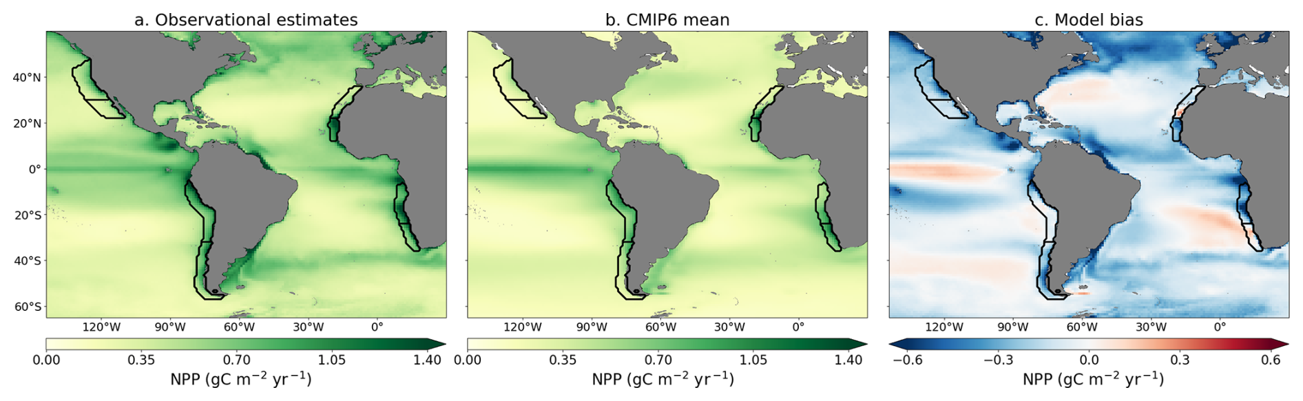
Figure 1 General ability of the CMIP6 models to simulate observed NPP in the EBUS albeit with certain biases. Time-averaged NPP (1998–2014) from observations (mean of five data products obtained combining ESA OC-CCIv4.1 ocean color observations with five different algorithms) (a), the CMIP6 multi-model mean (18 models) (b), and the difference between the two (simulated minus observed) (c). The four EBUS are indicated by black borders in each map, with the poleward and equatorward regions indicated by black lines at the latitudes of 30° N (CalCS), 22° N (CanCS), 32° S (HumCS), and 24° S (BenCS).

EBUS primary production is largely driven by the high availability of macro- and micronutrients in the euphotic zone (Carr and Kearns, 2003). These nutrients are supplied through intense coastal upwelling to surface layers, where they become accessible to phytoplankton (Bakun, 1990; García-Reyes et al., 2015). This process is primarily associated with offshore Ekman transport, induced by the alongshore equatorward winds that result from the atmospheric pressure gradient between high-pressure systems over subtropical ocean basins and low-pressure systems over adjacent land masses. In addition to this dominant mechanism, other physical processes also influence the supply of nutrients, such as cross-shore geostrophic transport near the coast (Oerder et al., 2015; Jacox et al., 2018) or Ekman pumping driven by wind-stress curl farther offshore (Bravo et al., 2016; Jacox et al., 2014).

Historically, perturbations to wind-induced upwelling have been thought to be the dominant drivers of the EBUS phytoplankton NPP response to climate change (Bakun, 1990; Sydeman et al., 2014; Bakun et al., 2015). Yet, projections of NPP remain uncertain, due to the interplay of multiple influencing factors, which can either reinforce or offset each other over varying time scales (Bograd et al., 2023; García-Reyes et al., 2015).

Numerous studies have focused on how future variations in alongshore wind-induced upwelling will affect NPP (Bakun, 1990; Rykaczewski and Checkley, 2008; Wang et al., 2015). Bakun's early theory (Bakun, 1990) suggested that global warming would enhance the ocean-land temperature and pressure gradients, strengthening coastal winds, intensifying upwelling, and increasing NPP. More recent research has extended this hypothesis, identifying a latitude-dependent NPP response within EBUS due to the potential future displacement of major high-pressure systems toward higher latitudes (Rykaczewski et al., 2015; Bograd et al., 2023). This shift, associated with the expansion of the Hadley cell (Lu et al., 2007; Grise and Davis, 2020) and the increase in the Southern Annular Mode (Gillett and Fyfe, 2013), could influence summertime alongshore winds, which are projected to intensify in the poleward regions of the EBUS and to weaken in the equatorward regions, potentially affecting the intensity and location of upwellings. Changes to large-scale atmospheric pressure systems may also affect the wind-stress curl in the EBUS, influencing the characteristics of induced upwelling (Pickett and Paduan, 2003; Rykaczewski and Checkley, 2008).

Alongside these mechanisms, shifts in the timing and duration of the upwelling season have been identified as potential contributors to total upwelling intensity, with future coastal upwelling trends showing heterogeneity throughout the year (Vázquez et al., 2023; Sousa et al., 2017). Earlier onset and prolonged duration of upwelling seasons are anticipated in the EBUS, attributed to variations in Ekman and geostrophic transport in the Pacific and Atlantic EBUS, respectively (Du et al., 2024). However, such changes have been found to have limited impact on total upwelling intensity compared to changes in vertical velocity. Moreover, future upwelling has also been shown to be modulated by shifts in geostrophic transport, associated with variations in sea surface height linked to global warming, which may offset the role of Ekman transport anomalies in some EBUS regions (Ding et al., 2021; Jing et al., 2023).

In addition to changes to the physical drivers of upwelling at depth, nutrient supply to the surface is further influenced by increased local stratification, which can limit transport efficiency, both by weakening mixing across the pycnocline and by causing a shallower source of upwelled waters (Roemmich and McGowan, 1995; Jacox and Edwards, 2011; Sousa et al., 2020).

Variations in the physical drivers of circulation and mixing, together with changes in the biogeochemical properties of source waters, modulate the nutrient supply to EBUS. Shifts in vertical nutrient transport have been shown to correlate well with changes in NPP (Du et al., 2024), with alterations in water column nitrate concentrations identified as critical in shaping future primary production (Jacox et al., 2024; Messié et al., 2009; Bristow et al., 2017; Jacox et al., 2016). Nitrate enrichment of upwelled waters, driven by changes in local processes (such as increased remineralization (Dussin et al., 2019; Rykaczewski and Dunne, 2010)) or basin-scale circulation (e.g. decreased ventilation at high-latitudes) has been shown to enhance productivity, compensating for changes in upwelling intensity and stratification (Rykaczewski and Dunne, 2010; Pozo Buil et al., 2021; Howard et al., 2020).

At present, the limited duration of observational records and associated measurement uncertainty hinder a robust assessment of climate impacts on EBUS NPP (Henson et al., 2010). Although studies have identified links between EBUS variability and natural low-frequency modes (Di Lorenzo et al., 2008; Cropper et al., 2014; Jacox et al., 2014), it remains difficult to disentangle anthropogenic influences from interannual to decadal fluctuations (Jacox et al., 2015; Bonino et al., 2019). Some studies have reported evidence of productivity trends over recent decades, with increases in certain regions and declines elsewhere (Kahru et al., 2009; Arístegui et al., 2009; Lamont et al., 2019; Weidberg et al., 2020). However, these findings often differ depending on the data source, and consistent long-term trends have not been established. For example, there is only medium evidence and medium agreement that primary production in the Canary Current has decreased (Arístegui et al., 2009; Demarcq, 2009). To address the limitations of observational records and understand potential changes of primary production in these systems, climate model simulations are increasingly employed.

Here we reevaluate the historical perspective that perturbations to upwelling favorable winds determine the EBUS NPP response to climate change. Using ESM simulations conducted within CMIP6 (O'Neill et al., 2016; Eyring et al., 2016) we assess the projected twenty-first century evolution of NPP across the four major EBUS under different Shared Socioeconomic Pathways (SSPs) (Riahi et al., 2017; Meinshausen et al., 2020). Specifically, we evaluate the extent to which projected changes in upwelling favorable winds are consistent with changes in vertical seawater velocities, upper ocean nutrient concentrations and NPP. The multi-model robustness of projections is evaluated and where NPP anomalies cannot be mechanistically explained by perturbations to upwelling-favorable winds, alternative drivers are explored, including changes to subsurface nitrate reservoirs and increasing ocean stratification.

2 Materials and methods

A multi-model ensemble approach was used to investigate the mechanisms driving changes in EBUS NPP under climate change. CMIP6 ESMs were analyzed, with the baseline period of historical simulations (1985–2014) compared with twenty-first century SSP projections (2015–2100).

2.1 Models

Model outputs were obtained from the CMIP6 archive hosted by the Earth System Grid Federation (ESGF). The selected ESMs simulate coupled physical (atmosphere, land, ocean, and sea ice) and biogeochemical processes (Table 1), allowing for a consistent evaluation of NPP changes and their potential drivers. The database underwent homogenization using distance-weighted average remapping: the resulting regridded files share a common horizontal resolution of 1° (360 × 180), while the vertical grid for each model retains its native discretization, which ranges from 40 to 75 levels. For each model, a single ensemble member was considered for each experiment (typically r1i1p1f1, sometimes r1i1p1f2 or r1i2p1f1), hence the potential influence of internal variability on projected changes was not considered.

(Ziehn et al., 2020)(Swart et al., 2019)(Christian et al., 2021)(Danabasoglu et al., 2020)(Danabasoglu et al., 2020)(Lovato et al., 2022)(Séférian et al., 2019)(Döscher et al., 2021)(Held et al., 2019; Dunne et al., 2020a)(Dunne et al., 2020b; Stock et al., 2020)(Boucher et al., 2020)(Hajima et al., 2020)(Müller et al., 2018; Mauritsen et al., 2019)(Mauritsen et al., 2019)(Yukimoto et al., 2019)(Tjiputra et al., 2020; Seland et al., 2020)(Tjiputra et al., 2020; Seland et al., 2020)(Sellar et al., 2019)

Table 1 The CMIP6 Earth System Models used, their atmospheric, ocean, and marine biogeochemistry components with the relative resolutions^a. The last column lists the experiments assessed for NPP projections (SSP5-8.5, SSP3-7.0, SSP2-4.5, SSP1-2.6), indicated for brevity only by their radiative forcing values in 2100 (8.5, 7.0, 4.5, 2.6). For SSP5-8.5, it is indicated whether a model is part of the ensemble subset used for full mechanistic analysis (✓) or not (X).

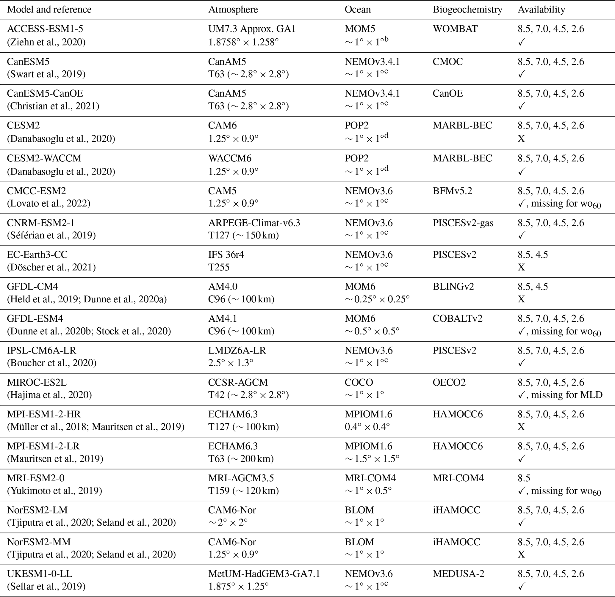
^a Resolution is expressed as longitude × latitude or by the truncation level used for the atmospheric component (symbol ∼ denotes nominal resolution). ^b Higher resolution near the equator (0.338°) and over the Southern Ocean (0.48°). ^c ORCA family tripolar configuration with refinement to $\mathrm{1}/\mathrm{3}$° close to the equator (Madec and Imbard, 1996). ^d Uniform resolution in the zonal direction (1.125°), varying in the meridional direction.

The evaluated scenarios were SSP1-2.6, SSP2-4.5, SSP3-7.0, and SSP5-8.5, with the latter specifically used to analyze the mechanisms driving climate-related NPP impacts, as the magnitude of projected changes is larger than in lower-emissions scenarios. While 18 CMIP6 models were used to assess changes in NPP, a subset of 13 models was selected for the full mechanistic analysis. This subset was based on the availability of complete datasets for all relevant variables over both historical and projection periods, ensuring internal consistency while maintaining ensemble diversity.

2.2 Model variables

The impact of climate change on EBUS phytoplankton activity was investigated through changes in NPP, a key indicator of ecosystem functioning and energy flow within marine ecosystems. NPP was vertically integrated over the full water column yet remains representative of upper-ocean layers, as productivity is largely confined to the well-lit shallow layers. In addition to NPP, variations in potential physical and biogeochemical drivers of NPP were also assessed (Table 2). Upwelling-favorable alongshore winds were evaluated using the equatorward and downward component of surface wind stress (τ_v), while upward seawater velocity at 60 m depth (wo₆₀) was used as a proxy for upwelling intensity. This particular depth was selected based on studies that have identified it as representative of the typical source layer (Messié et al., 2009; Chavez and Messié, 2009). Although the actual origin of upwelled waters varies in both time and space, backward particle tracking and sensitivity tests on nitrate supply have demonstrated that 60 m provides a reliable estimate.

Table 2 Overview of the variables used.

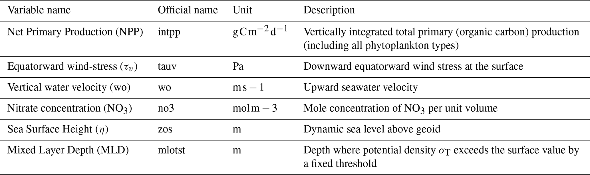
Nutrient analysis focused primarily on nitrate, as it has been shown to be the dominant limiting nutrient in EBUS (Messié and Chavez, 2015; Bograd et al., 2023; Jacox et al., 2024). NO₃ concentrations were assessed at three depths: the surface, where nutrients are directly consumed by phytoplankton; 60 m, where upwelled waters are supposed to originate from; and 200 m, which characterizes the regional subsurface nutrient reservoir. Variability at this deeper level may strongly influence future NPP trends (Rykaczewski and Dunne, 2010; Jacox et al., 2024).

The sea surface height (η), used for the geostrophic transport calculation, is the dynamic sea level above geoid, while the ocean mixed layer depth (MLD) is evaluated using the sigma-t (σ_t) criterion, where MLD is defined as the depth at which potential density exceeds the surface value by a model-specific threshold. This metric delineates the base of the well-mixed surface layer and is critical for understanding vertical mixing and nutrient entrainment.

2.3 Data processing

The eastern boundary upwelling systems were delineated using four of the 66 recognized Large Marine Ecosystems (Sherman and Duda, 1999; Sherman, 2015), ocean regions along continental coasts characterized by high primary productivity. In particular, the definitions of the EBUS spatial domains were associated with their relative oceanographic features, as each system included the associated equatorward surface eastern boundary current. Masks identifying these domains were obtained from the ISIMIP (Inter-Sectoral Impact Model Intercomparison Project (ISIMIP), 2024) repository, and have variable extents in longitude (widths from 4 to 9°) and latitude (lengths from 25 to 50°) (Fig. 1). The division of the masks into poleward (CalCS-P, CanCS-P, HumCS-P, and BenCS-P sub-EBUS) and equatorward (CalCS-E, CanCS-E, HumCS-E, and BenCS-E sub-EBUS) portions is based on the spatial patterns of ensemble-mean NPP anomalies.

Climate change impacts on NPP were assessed by computing anomalies, defined for each model as the difference between the projection and the respective values over the baseline period (1985–2014). Ensemble means of both time series and maps of anomalies were calculated, in order to determine dominant patterns across different model outputs. Time series were obtained using spatial averages within each EBUS mask, with weighted means applied to account for differences in grid cell area. Model uncertainty in the projections was evaluated by calculating the standard deviation across the ensemble for each SSP, while scenario uncertainty was assessed using the divergence between SSP trajectories. Spatial anomalies were computed by time averaging over the last 30 years of SSP simulations (2071–2100). Regions of consistent changes across the ensemble were identified, with high model agreement defined as at least 80 % of models aligning on the sign of future changes, as described in Arias et al. (2021).

To investigate the drivers of projected NPP changes, relationships between NPP and its potential drivers were evaluated. Within each EBUS mask, grid cells were classified based on the sign and coherence of anomalies between variable pairs–specifically, τ_v–NPP, τ_v–wo₆₀, wo₆₀–NO₃, and NO₃–NPP. For each variable pair, four outcomes exist (both variables increasing, both decreasing, one increasing while the other decreases, and vice versa) with each grid cell categorized accordingly. To ensure that only robust, ensemble-consistent relationships were retained, the classification was applied only if at least 50 % of ensemble members agreed on the relationship. This threshold is lower than that used for standard ensemble anomalies and was preferred over higher thresholds, as sensitivity tests showed that those would have resulted in an excessively large reduction of the agreement area due to the greater number of possible pairwise outcomes. This approach was extended to include three-variable relationships (τ_v–NO₃–NPP), where classifications were only applied if the anomalies of all three variables shared the same sign across the ensemble majority. It should be noted that, while this analysis assesses mechanistically the dynamics of EBUS changes, it does not account for potential non-linearities between variable pairs that may influence the magnitude of changes.

For the analysis of Ekman and geostrophic transports, the methodology outlined in Jacox et al. (2018) has been followed. The zonal Ekman transport, defined as the integrated near-surface transport directed 90° to the right (left) of the surface wind stress in the Northern (Southern) Hemisphere, is computed as:

$$\begin{array}{}\text{(1)}& U_{\text{ekm}}={\displaystyle \frac{{\mathit{\tau }}_v}{{\mathit{\rho }}_{\mathrm{0}}f}}\end{array}$$

where ρ₀ = 1025 kg m⁻³ is the seawater density, and f is the Coriolis parameter.

The cross-shore geostrophic flow is calculated as:

$$\begin{array}{}\text{(2)}& U_{\text{geo}}=-{\displaystyle \frac{g}{f}}{\displaystyle \frac{\partial \mathit{\eta }}{\partial y}}H\end{array}$$

where g is the gravitational acceleration, and H is the Ekman layer depth, set for simplicity at 30 m, a depth which has been shown to provide a robust approximation (Ding et al., 2021; Veitch et al., 2010).

2.4 Observational products

Observational net primary production estimates for the period 1998–2014 were obtained from Ryan-Keogh et al. (2023) which combines the ocean colour data product from the European Space Agency Ocean Colour Climate Change Initiative project (ESA OC-CCIv4.1) (European Space Agency (ESA), 2024), with five different algorithms: Eppley-VGPM (Eppley, 1972), Behrenfeld-VGPM (Behrenfeld and Falkowski, 1997), Behrenfeld-CbPM (Behrenfeld et al., 2005), Westberry-CbPM (Westberry et al., 2008), and Silsbe-CAFE (Silsbe et al., 2016). For surface equatorward wind stress, CMIP6 outputs were compared for the period 1998–2014 with the ERA5 reanalysis (European Centre for Medium-Range Weather Forecasts, 2019). For nitrate concentrations, data were obtained from the climatology (1965–2022) of the World Ocean Atlas 2023 (WOA; (Garcia et al., 2024)), using both surface and subsurface (200 m) NO₃ fields.

3 Results

3.1 Model evaluation

Historical observations of global NPP highlight the eastern boundary upwelling systems as highly productive regions (Fig. 1a). Over the historical period, the multi-algorithm mean indicates the highest average NPP in the BenCS, with a mean of about 0.99 $\mathrm{g}\mathrm{C}{\mathrm{m}}^{-\mathrm{2}}{\mathrm{d}}^{-\mathrm{1}}$, followed by the HumCS with 0.86 $\mathrm{g}\mathrm{C}{\mathrm{m}}^{-\mathrm{2}}{\mathrm{d}}^{-\mathrm{1}}$, the CanCS with 0.82 $\mathrm{g}\mathrm{C}{\mathrm{m}}^{-\mathrm{2}}{\mathrm{d}}^{-\mathrm{1}}$, and the CalCS with 0.54 $\mathrm{g}\mathrm{C}{\mathrm{m}}^{-\mathrm{2}}{\mathrm{d}}^{-\mathrm{1}}$. Productivity patterns show spatial variability, with peak values in localized regions where strong alongshore winds drive deep, nutrient-rich waters to the surface.

Comparison between the observational data and ensemble mean simulations for the same period shows that models capture the large-scale NPP variability and generally identify high productivity regions in EBUS (Fig. 1b), even if with a slight misrepresentation of the precise location of hotspots (especially in CanCS and BenCS). The difference between simulated and observed values (Fig. 1c) reveals some drawbacks, with models underestimating NPP–especially in coastal regions of high productivity. On average, models underestimate NPP by −0.23 $\mathrm{g}\mathrm{C}{\mathrm{m}}^{-\mathrm{2}}{\mathrm{d}}^{-\mathrm{1}}$ in the CalCS, −0.18 $\mathrm{g}\mathrm{C}{\mathrm{m}}^{-\mathrm{2}}{\mathrm{d}}^{-\mathrm{1}}$ in the CanCS, −0.23 $\mathrm{g}\mathrm{C}{\mathrm{m}}^{-\mathrm{2}}{\mathrm{d}}^{-\mathrm{1}}$ in the HumCS, and −0.26 $\mathrm{g}\mathrm{C}{\mathrm{m}}^{-\mathrm{2}}{\mathrm{d}}^{-\mathrm{1}}$ in the BenCS. These discrepancies may be attributed to limitations in model representations of wind dynamics, upwelling processes, or biogeochemical parameterizations (e.g. sedimentat interactions).

Assessing the ability of individual models to simulate historical mean states of NPP reveals both model-specific biases and spread within observational data products. Generally models capture values across the four EBUS, and the range of CMIP6 outputs is larger, yet comparable to that of the observations (Fig. S1 in the Supplement). Models that underestimate (or overestimate) NPP in one region generally show similar biases across the other systems. Mean states of nutrient and wind fields are also well reproduced by models. Simulated surface and subsurface (200 m) nitrate concentrations are generally consistent with observations at the EBUS scale, with observational data lying only outside the intermodel spread (i.e., beyond the whiskers extending to 1.5 × IQR) in the HumCS for surface NO₃ (Fig. S2a) and in the BenCS for 200 m NO₃ (Fig. S2b). Likewise, the CMIP6 ensemble captures the mean state of surface equatorward wind stress, with the ERA5 reanalysis product only outside intermodel spread in the CalCS-E (Fig. S3a).

Ultimately, this evaluation cannot confidently restrict the ensemble to the most “realistic” models. Identifying the best models is difficult due to large uncertainties in observational data, the short evaluation period and because historical outliers do not consistently remain outliers in future projections, preventing us from simply excluding them. Moreover, as it will be shown in the next section (Fig. S5), CMIP6 outliers are strongly dependent on the EBUS considered (CanESM5 for CalCS, IPSL-CM6A-LR for CanCS, CanESM5-CanOE for HumCS, and CanESM5-CanOE and ACCESS-ESM1-5 for BenCS). Thus, constraining the ensemble based on performance during the historical period is not straightforward and this evaluation section cannot be used to narrow projection uncertainty.

Generally models are able to capture historical trends for NPP and winds at the sub-EBUS scale. For NPP, in most regions, the simulated trends fall within the observational range (Fig. 2). Although CMIP6 models have limited confidence on signs of change, their spread is comparable to observational data. For surface equatorward wind stress, there is low confidence in the sign of historical trends, likely due to the strong influence of interannual and decadal variability during the study period. Nevertheless, the models perform well overall, with the observational product lying within the intermodel spread everywhere except the CalCS-P and BenCS-E regions (Fig. S3b).

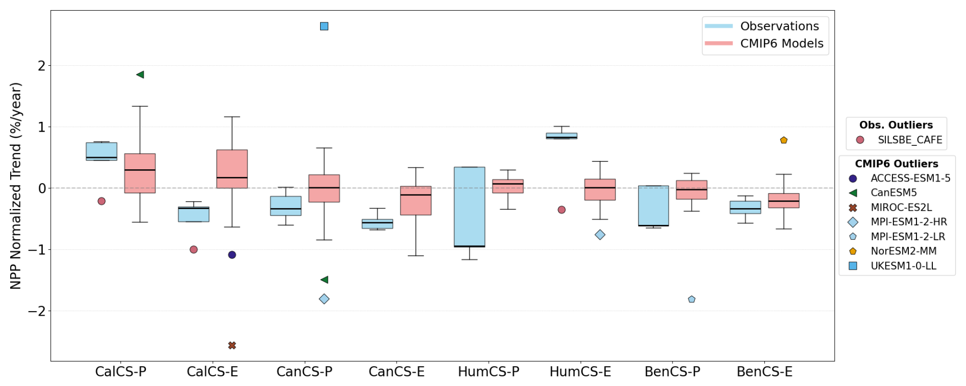
Figure 2 Distribution of historical (1998–2014) NPP trends across sub-EBUS from observational data products and the CMIP6 models. Box-and-whisker plots show the interquartile range (IQR), whiskers extend to 1.5 × IQR, and medians are indicated by thick black lines. Observational products are shown in blue and CMIP6 models in salmon. Colored markers show outliers for both observational and CMIP6 data.

3.2 NPP projections and associated uncertainties

Projected changes in net primary production under climate change reveal distinct patterns both across and within eastern boundary upwelling systems. An analysis of the multimodel mean time series of NPP, based on a 13 model ensemble (see selection criteria detailed in Materials and Methods), showed that only in the CanCS and HumCS the projected anomalies are non-negligible in magnitude and SSP-consistent in the direction of change (Fig. 3). Comparable results are obtained using the full CMIP6 ensemble (Fig. S4). By 2100, ensemble mean NPP is anticipated to decline in CanCS (between −7 %/−10 % under different SSPs), and to increase in HumCS (with larger anomalies for higher emission scenarios, ranging from +2 % under SSP1-2.6 to +7 % under SSP5-8.5). In contrast, ensemble mean anomalies remain close to zero under all SSPs in both CalCS and BenCS.

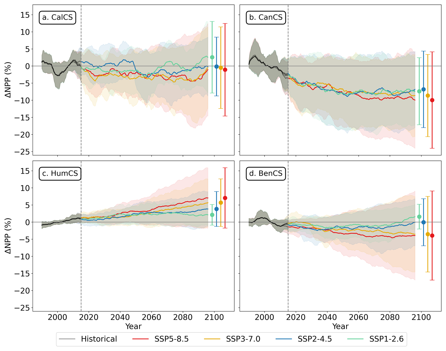
Figure 3 Diverse and uncertain NPP responses across EBUS. Historical (1985–2014, grey) and projected (2015–2100, colored) relative change in NPP for different SSPs using the selected models from the CMIP6 ensemble: ensemble means are indicated with solid lines, intermodel standard deviation with shaded regions. Colored vertical bars indicate, for each scenario, the intermodel standard deviation by the end of the century. A 10-year smoothing is applied.

Consensus on the sign of anomalies is larger in CanCS and HumCS, with most members projecting, respectively NPP decreases (11/13 models, Fig. S5b) and increases (8/13 models, Fig. S5c) under SSP5-8.5. In CalCS and BenCS, the intermodel spread includes both positive and negative future anomalies (7 increasing vs. 6 decreasing in CalCS, Fig. S5a; 6 increasing vs. 7 decreasing in BenCS, Fig. S5d). By the end of the 21st century, intermodel standard deviation is lowest for the HumCS (17 %), followed by the CanCS (26 %), CalCS (28 %), and BenCS (31 %). Across the other scenarios, in CalCS and CanCS intermodel spreads remain comparably large, while in BenCS and HumCS intermodel spreads decrease under lower-emissions scenarios.

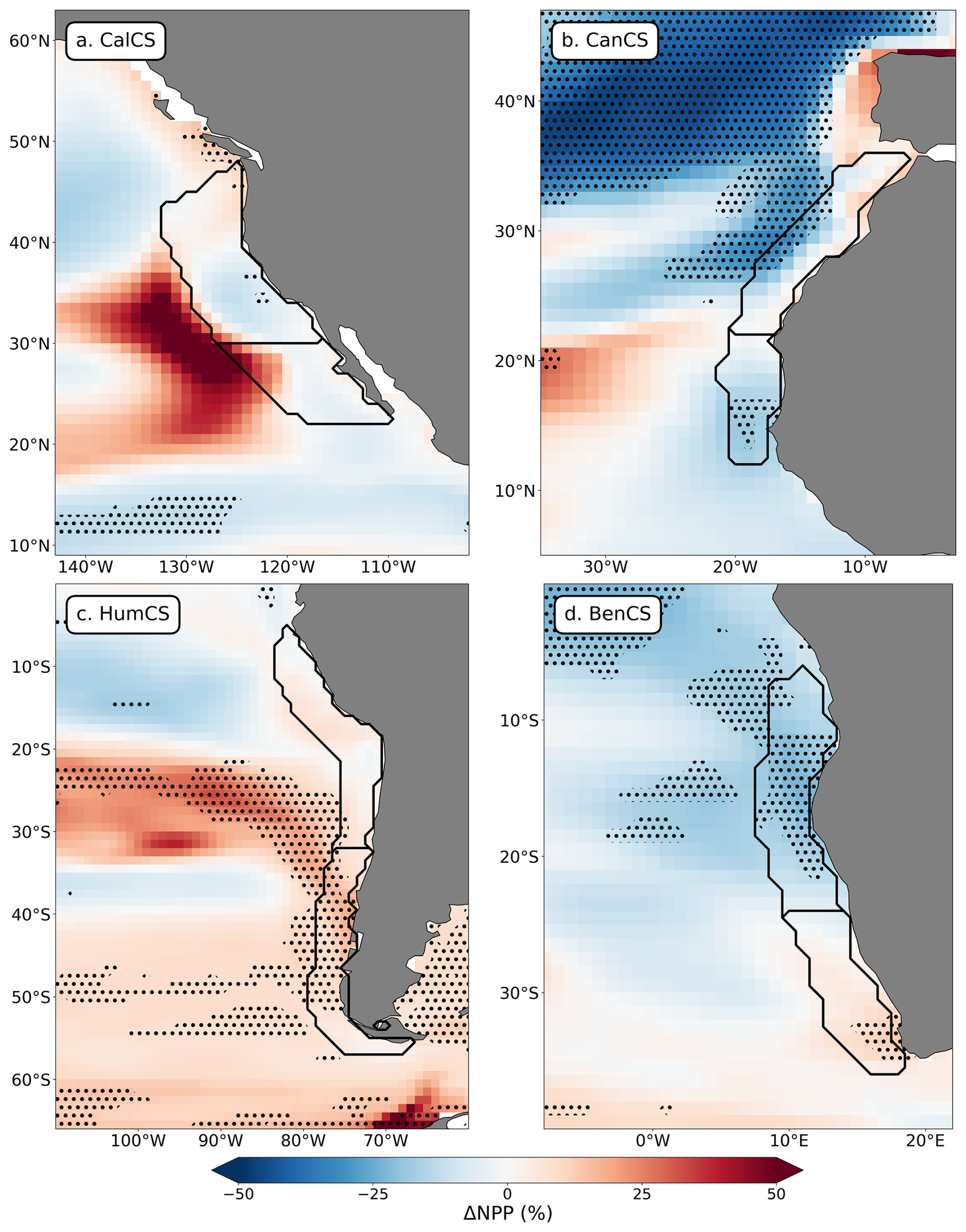
Figure 4 CMIP6 ensemble mean anomalies of NPP show regionally contrasting trends within individual EBUS. Ensemble mean (13 models) NPP anomalies (2071–2100 relative to 1985–2014) under SSP5-8.5 in the four eastern boundary upwelling systems. Stippling highlights areas of high model agreement. The poleward and equatorward sub-EBUS are indicated in each map by black lines at the latitudes of 30° N (CalCS), 22° N (CanCS), 32° S (HumCS), and 24° S (BenCS).

The high uncertainty in NPP projections at the EBUS scale arises from two main sources: intermodel differences and the compensation of positive and negative anomalies within individual EBUS regions. As a result, spatially heterogeneous but internally coherent signals are often masked when averaged over the entire EBUS domain (Fig. 3). At the sub-EBUS scale, however, CMIP6 models frequently exhibit consistent regional trends (Fig. S6). The coexistence of opposing anomaly patterns within a given EBUS therefore contributes substantially to the larger uncertainty diagnosed at the aggregated scale (Fig. 4). Under SSP5-8.5, the ensemble mean projects declining NPP in several regions, including the southern and central coastal sectors of the CalCS, the CanCS, the equatorward portion of the BenCS, and the northern limit of the HumCS. The most pronounced and robust declines are projected in CanCS-P and CanCS-E, where relative anomalies reach approximately −30 % and −20 %, respectively (Fig. 4b). Similarly, robust negative anomalies are simulated in BenCS-E, reaching up to −20 % (Fig. 4d), with 10 out of 13 models projecting decreasing trends in this region (Fig. S6h). Projected declines are weaker and less robust in other systems. In the CalCS, the strongest decrease occurs within the historically most productive region (CalCS-P; 30–40° N), where anomalies peak near −10 % (Fig. 4a). This is also the only CalCS sub-region characterized by relatively strong model agreement, with 8 out of 13 models simulating declining NPP trends (Fig. S6a). In the HumCS, negative ensemble mean anomalies at the equatorward boundary remain weak (−2 %) and lack robustness. Over the remainder of the HumCS, positive anomalies dominate, reaching up to +16 % around 40° S, with high intermodel agreement between 35 and 50° S. Likewise, robust positive anomalies are projected in BenCS-P, where NPP increases by up to +10 % (Fig. 4d), and 8 out of 13 models simulate positive trends (Fig. S6g). Outside the coastal band between 30 and 40° N, ensemble mean anomalies in the CalCS are spatially inconsistent among models (Fig. 4a), and uncertainty in CalCS-E remains primarily driven by intermodel variability (Fig. S6b). Overall, strong model agreement is restricted to only 20 % of the total EBUS area (Figs. 4 and S7).

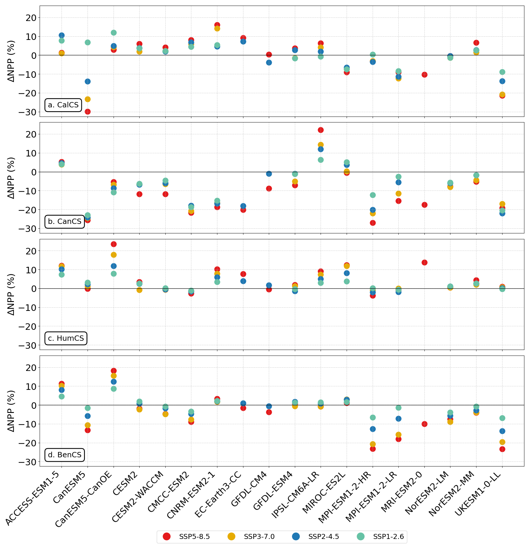
Figure 5 NPP anomalies exhibit greater model uncertainty than scenario uncertainty. For each CMIP6 model, each point represents the NPP anomaly, averaged over the final 30 years of simulations (2071–2100 relative to 1985–2014) and spatially averaged across the entire system domains, under the four SSPs.

We find that model uncertainty across CMIP6 is larger than scenario uncertainty. While there is often model disagreement on the overall direction of anomalies, for individual members the sign of productivity change remains generally consistent across different SSPs, with larger magnitude of changes under higher emission pathways (Fig. 5). This suggests that NPP projections are more sensitive to model choice than emission scenarios. Moreover, analysis of spatial NPP anomalies under SSP3-7.0, SSP2-4.5, SSP1-2.6 suggests that patterns are not scenario-dependent, but rather reflect changes in the underlying processes that drive productivity in these regions (Figs. S8–S10). Directions of changes are spatially consistent across all SSPs, as the same areas are projected to experience similar productivity trends, with lower emissions pathways showing smaller magnitudes of variation. The level of agreement and the regions of robust changes remain generally the same across scenarios.

3.3 Drivers of NPP changes

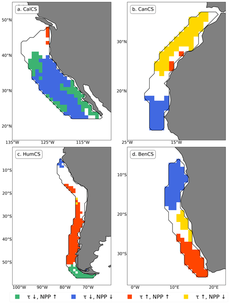
Projected declines in NPP from the CMIP6 ensemble mean are linked to local weakening of alongshore winds in central CalCS and in the equatorward CanCS and BenCS (Fig. 6). Co-located decreases in τ_v and NPP are consistently projected in the central and southern CalCS, in the equatorward Canary and Benguela systems, and at the northern edge of HumCS (28.4 % of total EBUS area), while increases are projected in the poleward sectors of HumCS and BenCS (20.1 %). In the remaining regions the two variables either do not show significant relationships (28.4 %), or change in opposite directions, with increasing (decreasing) NPP associated with weaker (stronger) τ_v in 9.8 % (13.3 %) of the EBUS area. The influence of seasonality on this finding is limited, as the same analysis obtained for summer data (months of June–August and December–February, respectively in the Northern and Southern Hemisphere) results in similar projected relationships between NPP and τ_v anomalies (Fig. S11). The main difference is observed in the poleward expansion, across all EBUS, of regions of consistently decreasing τ_v and NPP, covering 38.7 % of the total EBUS area compared to 28.4 % in the annual case. In the CanCS, summer weakening of τ_v extends across the entire system, as the region of increasing τ_v shifts further north, outside its boundaries.

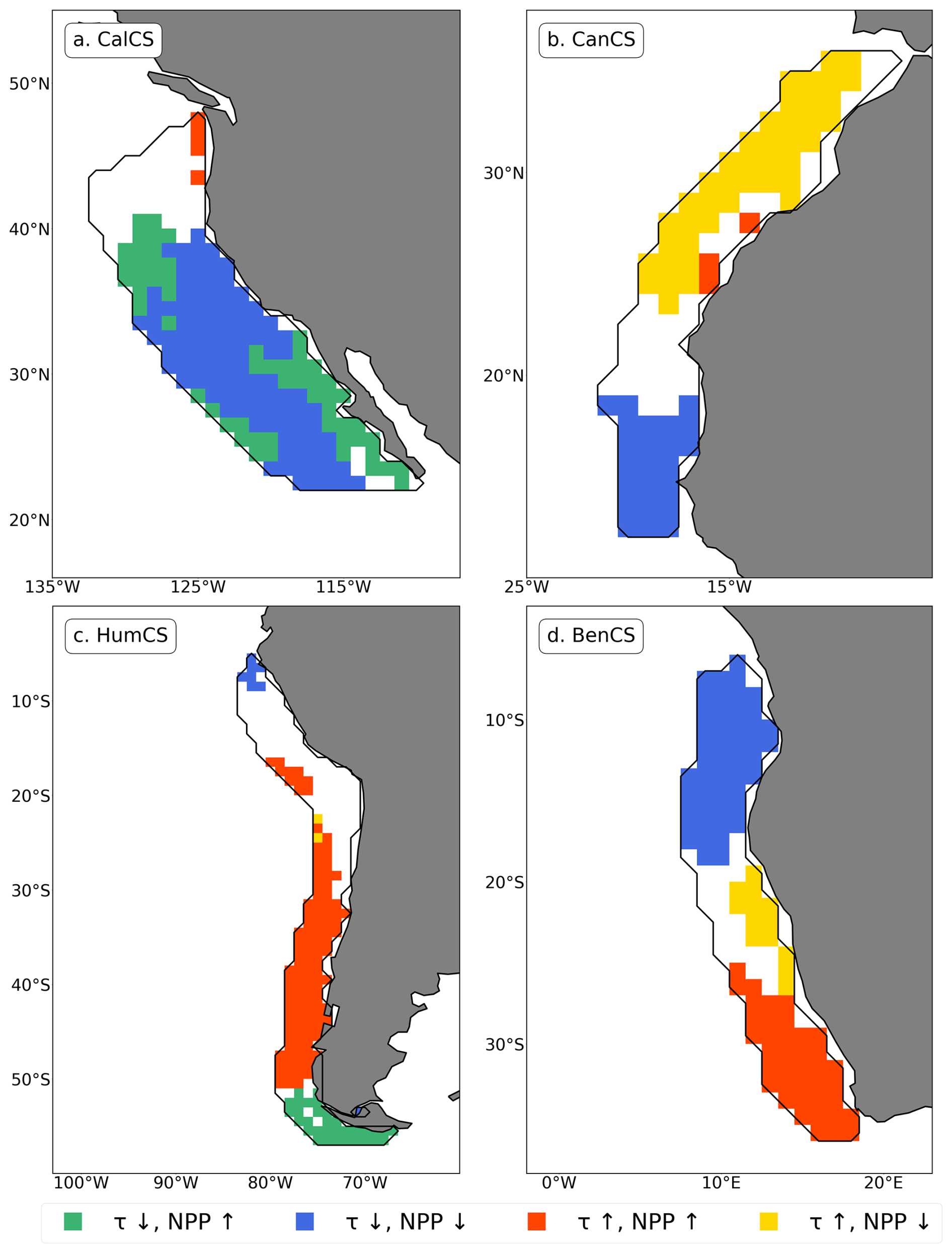
Figure 6 Variable relationships between projected anomalies in τ_v and NPP within and across EBUS. Signs of twenty-first century co-localized anomalies in τ_v and NPP under SSP5-8.5 (2071–2100). Grid cells are colored if there is ≥ 50 % model agreement.

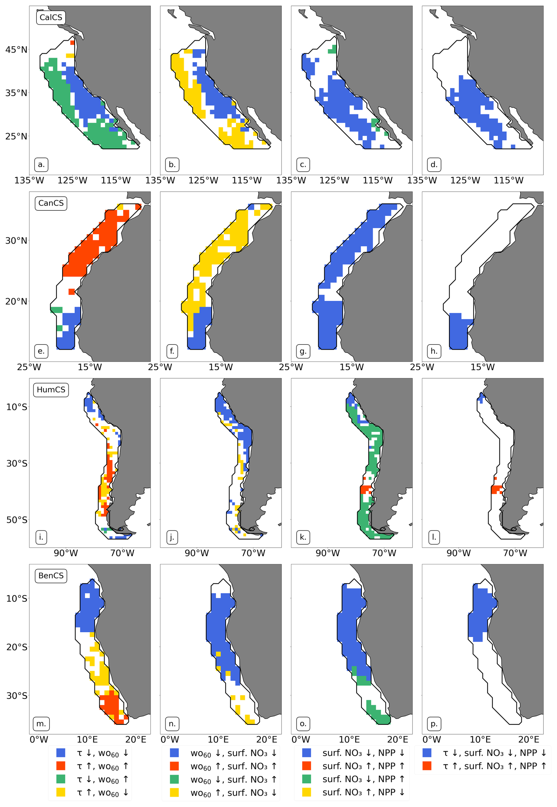
Figure 7 Consistent decreases of τ_v, surface NO₃, and NPP in the equatorward portions of CanCS and BenCS and in central CalCS, variable relationships elsewhere. Signs of twenty-first century co-localized anomalies among key variables under SSP5-8.5 (2071–2100). Grid cells are colored if there is ≥ 50 % model agreement on the relationship between anomalies of: τ_v vs. wo₆₀ (first column), wo₆₀ vs. surface NO₃ (second), surface NO₃ vs. NPP (third), and τ_v, surface NO₃, and NPP combined (fourth).

Alongshore winds are primary drivers of NPP changes only in the equatorward portions of CanCS and BenCS, and in the central CalCS (Fig. 7d, h, l, and p). In these areas, models project simultaneous decreases in τ_v, surface NO₃, and NPP, while elsewhere this mechanistic chain connecting coastal wind stress to primary productivity either breaks down or is inconsistent. When the same analysis also includes changes in wo₆₀, the regions showing consistent declines across all four variables shrink, especially in the CalCS, where they localize around a coastal spot between 30–40° N, potentially due to lower model availability for the vertical velocity variable (Fig. S12).

Coincident twenty-first century declines in alongshore winds, seawater vertical velocity, nitrate concentrations, and primary productivity–reflecting the classical upwelling-driven productivity mechanism–are projected in only 25 % of the total EBUS area under SSP5-8.5. This limited overlap highlights the role of additional processes in shaping the NPP response to climate change across these systems.

Upwelling changes are associated with alongshore wind stress in only some sectors of EBUS, as their relationship varies regionally (Fig. 7a, e, i, and m). Upwelling intensity is consistently projected to decrease together with alongshore wind in the equatorward regions of CanCS and BenCS and in the coastal spot of central CalCS, while in the poleward CanCS, both wind strength and upwelling are projected to increase (SSP5-8.5 anomalies of τ_v and wo₆₀ are provided, respectively in Figs. S13 and S14). Elsewhere, upwelling intensifies despite τ_v weakening (in the offshore area of CalCS) or no significant relationship is projected between the two variables (in the poleward areas of BenCS and HumCS).

Moreover, while the upwelling weakening is associated with future declines in surface nitrate, regions of future wo₆₀ intensification do not show corresponding NO₃ changes (Fig. 7b, f, j, and n). In the equatorward areas of CanCS, HumCS and BenCS and in the central CalCS negative wo₆₀ anomalies are consistently associated with reduced surface nitrate (36 % of total EBUS area). Elsewhere, despite the intensified upwelling, the CMIP6 ensemble projects a general surface NO₃ decline (31 % of total EBUS area).

Finally, while NPP and surface NO₃ are consistently projected to both decrease in some EBUS areas, positive NPP anomalies are not linked to NO₃ increases (Fig. 7c, g, k, and o). The nitrate decrease is consistently associated with reduced NPP everywhere except in the offshore and northern California system, where model agreement is low (in 46 % of total CalCS area), and in the poleward sector of BenCS and across most of HumCS, where NPP increases (where this relationship is consistent in 16 % of the BenCS and in 63 % of HumCS areas, respectively).

4 Discussion

Projected directions and magnitudes of EBUS NPP changes are broadly in line with earlier findings from CMIP5 (Cabré et al., 2015) and similar to CMIP6 analysis (Bograd et al., 2023). Future NPP declines in the equatorward regions of CanCS and BenCS and in the coastal area of central CalCS are consistent with a weakening of upwelling-favorable winds, while, outside of these regions, contributions from other factors dominate. The following discussion aims to clarify the underlying mechanisms responsible for these spatial variations.

4.1 Geostrophic transport and wind-stress curl may affect future upwelling

While CMIP6 models consistently indicate that weaker alongshore winds result in reduced productivity, their strengthening does not directly induce higher NPP (Figs. 6 and 7). Upwelling is primarily driven by alongshore wind stress in central CalCS and in the equatorward areas of CanCS and BenCS (decreasing τ_v and wo₆₀), and in the poleward area of the CanCS (increasing τ_v and wo₆₀). Outside these regions, τ_v and wo₆₀ show either inconsistent relationships (in the poleward BenCS and HumCS) or opposite directions of changes (wo₆₀ intensifies despite τ_v weakening around the coastal CalCS area between 30–40° N). This indicates that vertical water velocity is influenced by additional physical mechanisms beyond the alongshore wind forcing.

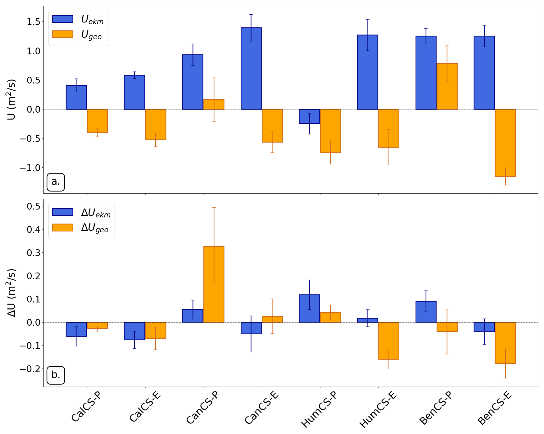
Figure 8 Relative contributions of Ekman and geostrophic transports in EBUS. Ensemble mean (13 models) Ekman and geostrophic transports in the sub-EBUS computed according to Eqs. (1) and (2), respectively, for historical (1985–2014) (a), and anomalies (2071–2100 relative to 1985–2014) (b).

Geostrophic transport changes can modulate upwelling by counteracting wind-driven changes in certain EBUS areas (Fig. 8). Consistent with previous studies (Jacox et al., 2018, 2024), we find that historical ensemble mean Ekman and geostrophic transport generally oppose each other (Fig. 8a), with positive Ekman transport (offshore, inducing upwelling) and negative (and smaller-magnitude) geostrophic transport (onshore, inducing downwelling) in most regions. Projected ensemble mean anomalies of the Ekman and geostrophic transport reinforce each other across most sub-EBUS domains (Fig. 8b). However, in some regions the projected ensemble mean changes diverge, offsetting each other, as shown also by Jing et al. (2023) and Du et al. (2024). Analysing colocalised anomalies in Ekman and geostrophic transport under SSP5-8.5 reveals that, in the central HumCS and BenCS-P regions, these transports tend to vary in opposite directions (Fig. S15). This is likely to contribute to the weak correspondence between wind and vertical velocity changes in these regions and partially explains the projected changes in wo₆₀ in the BenCS-P, but provides limited additional insight in the HumCS, where vertical velocity remains highly variable. Moreover, the mismatch between projections of decreasing τ_v and increasing wo₆₀ around the localized spot between 30–40° N of the CalCS aligns with the potential role of wind-stress curl in determining offshore upwelling, > 50 km from the coast (Bograd et al., 2023; Jacox et al., 2014).

4.2 Stratification and subsurface nutrients modulate nutrient supply

Projected twenty-first century changes in upwelling intensity are insufficient to explain surface ocean NO₃ anomalies in the EBUS. Regions of enhanced upwelling intensity do not consistently show corresponding surface nitrate increases, as upper ocean nutrient supply is also impacted by perturbations to water column stratification and subsurface nutrient reservoirs.

In the poleward portion of the CanCS, increased stratification and a shallower mixed layer depth likely drive NPP decline despite intensified upwelling (Fig. 7e, f, g, h). Although upwelling of cold, deep waters typically offsets warming effects in EBUS (García-Reyes et al., 2015), a consistent MLD shoaling is projected everywhere with the exception of local HumCS regions (not shown). MLD shoaling is particularly pronounced in the poleward CanCS (Fig. 9). The MLD in this region is historically deeper (∼ 60 m) than in other EBUS and is expected to shoal by substantially more (∼ 20 m shoaling). Under such conditions, enhanced stratification may overcompensate upwelling intensification, reducing vertical mixing and surface nutrient supply, and lowering productivity. Similar trends have been projected off the nearby Iberian Peninsula (Sousa et al., 2020), reinforcing this finding. Shoaling of upwelling source depth has also been linked with increased stratification, potentially resulting in waters with lower nutrient concentrations reaching the surface (Jacox and Edwards, 2011), however water parcel trajectory analysis was beyond the scope of this study.

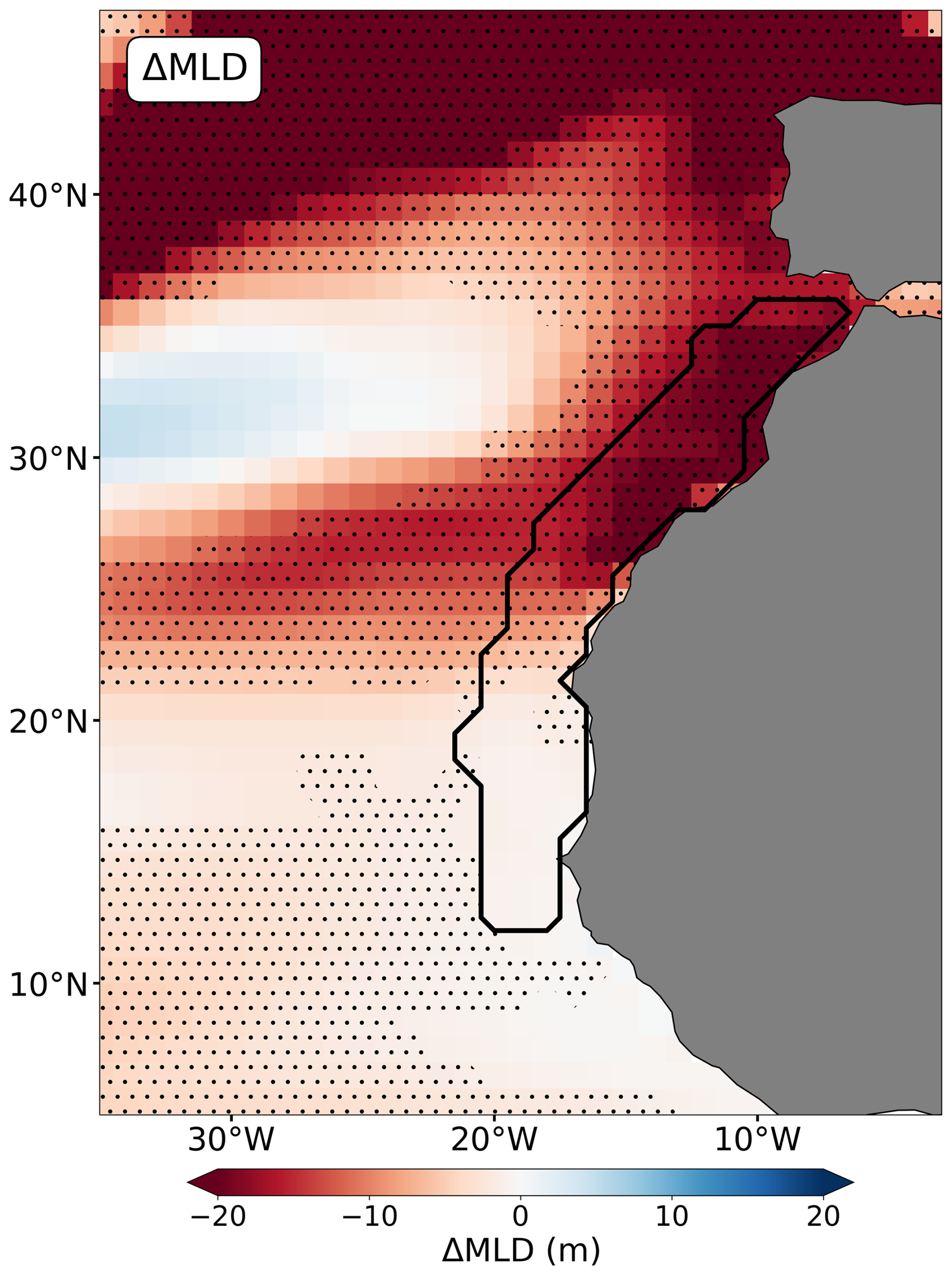
Figure 9 Strong mixed layer depth shoaling in the poleward CanCS. Ensemble mean (12 models) MLD anomalies (2071–2100 relative to 1985–2014) under SSP5-8.5 in the Canary EBUS. Stippling highlights areas of high model agreement.

In addition to enhanced stratification, simulated changes in subsurface nitrate reservoirs may be as important as changes in upwelling intensity in determining EBUS NPP projections. Euphotic zone nutrient supply is a consequence of both water mass transport and the concentration of nutrients associated with those waters. The impact of subsurface nitrate anomalies on NPP is limited because perturbations do not consistently propagate to shallower waters, and because, where they do, NO₃ availability may not be the primary driver of NPP variability (Echevin et al., 2008). Consistent declines in 200 m NO₃ and NPP are projected in central coastal California and in equatorward CanCS and BenCS (Fig. S16). Reduced nitrate throughout the water column contributes to the NPP decrease, reinforcing the effect of weaker wind stress and upwelling intensity. Surface nitrate reductions may also be associated with the impoverishment of upwelled waters in the offshore California system (Fig. S17), however impacts on NPP are uncertain. While NO₃ is projected to increase around 200 m in this region (Fig. S18a), these waters do not reach the typical source depth (60 m), potentially due to enhanced stratification and the consequent shoaling of the upwelling source depth in the area. The projected negative anomalies in upwelled waters (Fig. S19a) result in reduced nutrient supply despite enhanced upwelling (Fig. 7b). Contrary to earlier findings indicating that source water nutrient content is the dominant driver of productivity in the CalCS (Rykaczewski and Dunne, 2010; Jacox et al., 2024), the CMIP6 ensemble shows inconsistent links between source water NO₃ concentrations and NPP, potentially due to the greater model ensemble size. In poleward HumCS and BenCS, lower nitrate supply is primarily driven by nutrient-poor upwelling, but the effect on NPP appears limited (Fig. S16). This could be due to historically low nitrate limitation in these areas, with future productivity more influenced by the relaxation of light limitation associated with the shoaling of the mixed layer, an effect highlighted in studies on seasonal NPP variability (Echevin et al., 2008; Vergara et al., 2017). It should be noted that while this study focuses on bottom-up control associated with nitrate supply to the euphotic zone, additional factors may shape future EBUS productivity. Specifically, co-limitation by nutrients such as iron (Browning and Moore, 2023; Echevin et al., 2008; Chavez and Messié, 2009), or top-down control by zooplankton grazing (Calbet and Landry, 2004; Slaughter et al., 2006) could be relevant drivers of NPP.

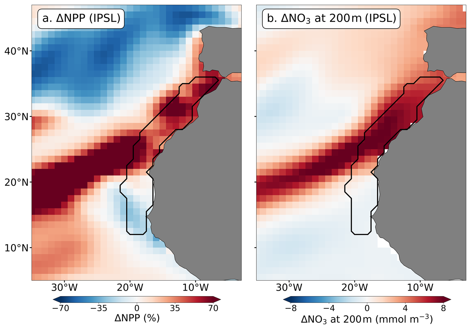
Figure 10 Evidence that subsurface nitrate increases can enhance projected NPP in the CanCS. IPSL-CM6A-LR projected anomalies (2071–2100 relative to 1985–2014) of NPP (a) and 200 m NO₃ concentrations (b) under SSP5-8.5 in the Canary EBUS.

We note that subsurface nitrate anomalies remain a key factor influencing NPP projections for individual models. For example, IPSL-CM6A-LR projects a relative NPP increase of more than 50 % by the end of the century over the Canary EBUS region north of 20° N (Fig. 10a), diverging from the ensemble mean, which projects a NPP decrease of about 7 % in this region. This divergence can be attributed to an increase in subsurface NO₃ concentrations in the IPSL model (mean anomaly of about 6.2 mmol m⁻³, Fig. 10b), which is more than double the ensemble mean (approximately 2.4 mmol m⁻³). This relatively high nitrate increase could be linked to nitrogen fixation, which has been shown to substantially increase in this model (Bopp et al., 2021). Enhanced diazotrophy in oligotrophic regions outside of the Canary EBUS, could lead to higher subsurface nitrate concentrations inside the system due to nutrient-rich water transport at depth.

5 Conclusions and Perspectives

The uncertainties associated with CMIP6 NPP projections in the four major EBUS stem from the complex interplay of multiple factors. This study highlights that the traditional paradigm of wind-driven upwelling perturbations determining future NPP changes only holds in 25 % of EBUS areal extent (in central CalCS and in equatorward portions of the CanCS and BenCS). Elsewhere, changes in additional mechanisms, both physical – geostrophic transport, wind-stress curl, stratification – and biogeochemical – subsurface nutrient reservoirs – are required to explain NPP responses in these ecologically and economically highly productive systems.

Assessing future NPP is complicated by the diverse spatial and temporal scales characterizing the underlying processes, which may exhibit non-monotonic behaviors or delayed responses (Jacox et al., 2016). While the atmosphere rapidly reacts to climate forcing, ocean inertia causes delayed changes in seawater properties. Natural variability, especially low-frequency modes such as El Niño-Southern Oscillation or the Pacific Decadal Oscillation, may influence EBUS NPP, hindering the ability to distinguish anthropogenic impacts (Sydeman et al., 2014; Jacox et al., 2015). Moreover, under projections beyond the typical end-of-century horizon, basin-scale feedbacks may alter properties of source waters feeding upwelling systems (e.g. through nutrient trapping (Moore et al., 2018)). In the EBUS, the effects of such changes are potentially further delayed, as the mean age of source waters can be decades to centuries (Resplandy et al., 2013; Bakun et al., 2015).

Although the CMIP6 Earth System Models used in this study offer a large-scale framework for assessing changes in EBUS NPP, their relatively low spatial resolution introduces certain limitations. ESMs may poorly represent coastal upwelling and fine-scale features such as mesoscale eddies or coastal trapped waves (Sylla et al., 2022; Small et al., 2015; Chang et al., 2023; Jing et al., 2023). Nevertheless, these global models permit the simulation of large-scale ocean and atmosphere dynamics at feasible computational cost. Given that the CMIP6 models indicate that large-scale processes extending beyond EBUS regions can influence local biogeochemical conditions, it is important that EBUS-specific regional ocean models are forced with boundary conditions derived from such global models to ensure consistency.