Water, carbon, and light use efficiencies in an old hemiboreal coniferous forest: nine-year patterns under hydroclimatic variability

Hemiboreal forests bridge boreal and temperate biomes by combining functional and compositional features of both and playing a key role in regional carbon and water cycling. Water (WUE), carbon (CUE), and light (LUE) use efficiencies provide integrative indicators of how effectively ecosystems convert available resources into carbon uptake, yet their long-term dynamics and controlling factors remain poorly explained in hemiboreal forests. We analysed nine consecutive growing seasons (2016–2024) of eddy covariance measurements from an old upland hemiboreal coniferous forest in southern Estonia to quantify WUE, CUE, and LUE and to identify their controls at daily and growing-season scales and along a standardized precipitation-evapotranspiration index (SPEI) defined hydroclimatic gradient.

Growing-season air temperature and vapour pressure deficit (VPD) increased over the study period. Despite this trend, WUE remained generally stable across years, with only one deviating growing season (2022) linked to intensified carbon uptake over a shorter season length. In contrast, CUE exhibited pronounced variability among growing seasons, driven primarily by changes in net ecosystem production and respiration dynamics. LUE was remarkably stable and showed no indication of age-related decline.

At the daily scale, VPD controlled WUE and LUE, whereas photosynthetically active radiation exerted dominant control over CUE. Along the hydrometeorological gradient, all three resource use efficiencies responded non-linearly, but WUE and LUE remained generally stable, while CUE was the most variable metric and reflected shifts in the balance between carbon uptake and respiratory losses.

Together, these results reveal differentiated sensitivities of ecosystem efficiencies to atmospheric drying and identify CUE as the most responsive indicator of hydroclimatic variability. Our findings provide new insight into the functional stability and potential thresholds of hemiboreal coniferous forests undergoing climate change.

1 Introduction

Hemiboreal forests are transitional ecosystems located between the boreal and temperate climate zones (Ahti et al., 1968; Hytteborn et al., 2005; Sjörs, 1963). These forests are mainly distributed across Northern Europe, the southern taiga of Russia, North America, and Northern Asia (Ahti et al., 1968; Brandt, 2009). Northern European hemiboreal forests are characterized by the coexistence of boreal coniferous and deciduous species, including Pinus spp., Picea spp., Betula spp., Populus spp., with temperate broadleaved species such as Quercus spp., Tilia spp., Fraxinus spp., Ulmus spp., Carpinus spp., Acer spp. (Manton et al., 2025; Nilsson, 1992). Within this mixed regional flora, boreal conifers remain a defining structural and functional component of many hemiboreal stands (FOREST EUROPE, 2026; Lee et al., 2023; Lindbladh et al., 2014; Petrokas et al., 2020).

Beyond their structural and functional importance, conifer-dominated hemiboreal forests in Northern Europe contribute to climate regulation through carbon uptake and storage (Jansons et al., 2025; Ķēniņa et al., 2019; Uri et al., 2022b). These forests store considerable amounts of carbon in biomass and soils and can function as net carbon sinks at both stand and regional scales (Bārdule et al., 2021; Ke et al., 2025; Rogozin et al., 2026). However, ongoing warming and atmospheric drying observed across northern forest regions can reduce tree growth, intensify water limitation, and alter the balance between carbon uptake and respiratory carbon losses (Krasnova et al., 2022; Mirabel et al., 2023; Restaino et al., 2016; Wu et al., 2012b). These effects may be particularly important for conifer-dominated hemiboreal stands, where boreal tree species occur toward the warmer and drier end of their climatic ranges (Ahti et al., 1968; D'Orangeville et al., 2018; Lindroth et al., 2020). Assessing whether these forests can maintain their carbon sink function under increasing climatic variability, therefore, requires an integrated understanding of the carbon, water, and energy exchanges (Jarvis and McNaughton, 1986; Sellers et al., 1997).

Resource use efficiencies (RUEs) provide integrative indicators of these coupled processes by relating ecosystem carbon uptake or retention to the use of water, assimilated carbon, and available light. At the ecosystem scale, water use efficiency (WUE) describes carbon uptake relative to water loss (Farquhar et al., 1982; Keenan et al., 2013), carbon use efficiency (CUE) represents the fraction of assimilated carbon retained after ecosystem respiration (DeLucia et al., 2007; Kutsch and Kolari, 2015; Waring et al., 1998), and light use efficiency (LUE) describes carbon uptake relative to available photosynthetically active radiation (Liu et al., 2019; Monteith, 1972; Stocker et al., 2018). Analysed together, these metrics help distinguish whether changes in ecosystem functioning arise primarily from water limitation, respiratory carbon losses, or constraints on light utilization. They are therefore particularly useful for assessing forest responses to rising CO₂, altered precipitation regimes, atmospheric drying, and more frequent drought (Guerrieri et al., 2016; Keenan et al., 2013; Stocker et al., 2018).

Despite numerous studies of RUEs dynamics and their relationships with environmental factors in boreal and temperate coniferous forest ecosystems (DeLucia et al., 2007; Gong et al., 2022), considerably less is known about forests in the Northern European hemiboreal zone. Relevant studies are available from nearby northern European coniferous forests. In Sweden, daytime air temperature was identified as a major driver of LUE variability (Lagergren et al., 2005). At the Hyytiälä station in southern Finland, LUE increased linearly with the aerosol-induced diffuse radiation fraction, with a substantially stronger response in mixed forests than in coniferous stands (Ezhova et al., 2018). A 17-year assessment at the same Finnish site showed that ecosystem-scale WUE remained relatively stable despite substantial variability in meteorological conditions among growing seasons (Launiainen et al., 2022), whereas extreme summer drought reduced WUE because photosynthesis was suppressed more strongly than evapotranspiration (ET) (Gao et al., 2017). Although these studies provide important regional context, they have generally focused on individual efficiency metrics or younger forest stands. Consequently, the long-term dynamics and environmental controls of multiple RUEs in old-growth coniferous forests remain poorly understood, especially in the Baltic hemiboreal region, where no comparable studies have been conducted.

In this study, we address this knowledge gap by examining nine consecutive growing seasons (2016–2024) of eddy covariance (EC) measurements from an old upland hemiboreal coniferous forest. Our study objectives are: (i) to quantify WUE, CUE, and LUE across the nine growing seasons, (ii) to examine their daily and growing-season variations and to determine the main environmental drivers controlling these changes, (iii) to analyse changes in RUEs in response to variations in hydrometeorological conditions.

Our study provides valuable insights for sustainable forest management. It advances the understanding of how transitional ecosystems function and contributes to global biogeochemical cycles, while also offering a knowledge base for climate and forestry policy.

2 Materials and Methods

2.1 Site description

The study site is located in southern Estonia (58.0236° N, 26.0708° E) at the Soontaga forest research station (Fig. 1).

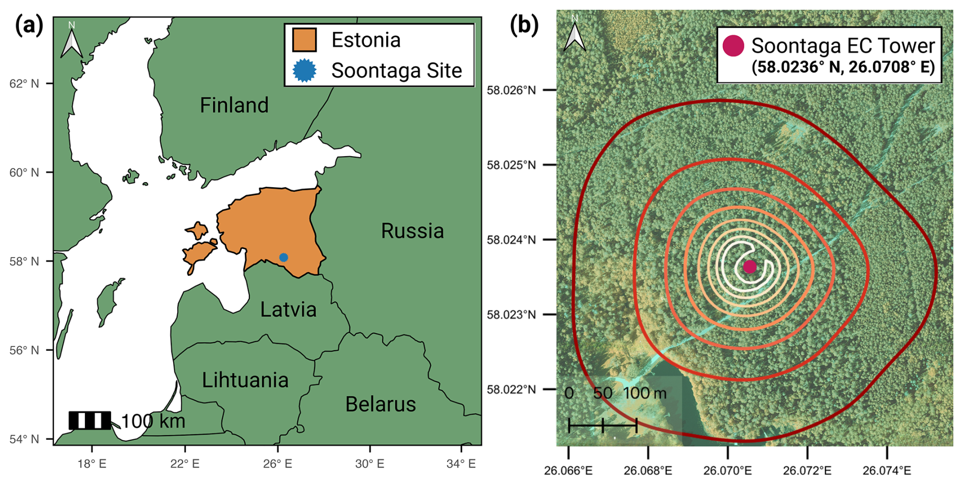
Figure 1 Location of the Soontaga eddy covariance (EC) site and modelled flux footprint. (a) Location of Estonia (orange) in northern Europe and the Soontaga study site (blue point). (b) Orthophoto of the Soontaga forest research station showing the EC tower (magenta point; 58.0236° N, 26.0708° E) and 10 %–80 % cumulative flux footprint contours for 2016–2024 (inner to outer) derived with the Flux Footprint Prediction (FFP) parameterisation (Kljun et al., 2015). Country boundaries were obtained from Natural Earth (Kelso and Patterson, 2009); the orthophoto background was obtained from the Estonian Land Board Geoportal (Orthophoto 16 December 2025, Republic of Estonia Land and Spatial Development Board).

The Soontaga study site (EE-Stg) is located in an old coniferous forest stand, with pine trees up to 230 years old. The canopy layer is dominated by Scots pine (Pinus sylvestris L.), with Norway spruce (Picea abies L. Karst) forming the secondary layer. According to the 2016 forest inventory data, the upper-canopy species composition by growing stock volume in the southern and central parts of the footprint consisted of approximately 98 % Scots pine and 2 % Norway spruce. Scots pine had a mean height of 32 m, a mean diameter at breast height (DBH) of 46 cm, and a basal area of 22.8 m² ha⁻¹, whereas Norway spruce had a mean height of 25 m, a mean DBH of 30 cm, and a basal area of 0.5 m² ha⁻¹. The secondary layer consisted of Norway spruce with a mean height of 17 m, a mean DBH of 16 cm, and a basal area of 2.0 m² ha⁻¹. According to the 2021 inventory, the species composition by growing stock volume in the northern part of the footprint consisted of approximately 80 % Scots pine, 19 % Norway spruce, and 1 % birch (Betula pendula). Scots pine had a mean height of 25 m, a mean DBH of 24 cm, and a basal area of 22.3 m² ha⁻¹, whereas Norway spruce had a mean height of 17 m, a mean DBH of 16 cm, and a basal area of 6.8 m² ha⁻¹. Birch had a mean height of 25 m, a mean DBH of 22 cm, and a basal area of 0.3 m² ha⁻¹ (Estonian Environment Agency, 2026). The understorey mainly consists of dwarf shrubs such as lingonberry (Vaccinium vitis-idaea L.) and blueberry (Vaccinium myrtillus L.), along with mosses like red-stemmed feathermoss (Pleurozium schreberi) and glittering woodmoss (Hylocomium splendens). In 2015, mean ground vegetation biomass was estimated at 6.40 ± 0.46 t ha⁻¹ following the methods described by Uri et al. (2022a). The soil in the footprint area is classified as endogleyic albic podzol, typical for dry, sandy upland sites with a low water table. A more detailed site description is available in a publication by Rogozin et al. (2026).

2.2 Instrumentation and environmental measurements

CO₂ concentrations were measured with an LI-7200 enclosed-path gas analyser (LI-COR Biosciences, Lincoln, NE, USA), while three-dimensional wind speed was recorded using a Metek uSonic-3 Class A ultrasonic anemometer (METEK GmbH, Elmshorn, Germany). All parameters were sampled at a frequency of 10 Hz, synchronized and stored in a CR3000 datalogger (Campbell Scientific Inc., Logan, UT, USA). Measurements were conducted at a height of 39 m, approximately 7 m above the forest canopy. The LI-7200 flow rate was maintained between 15 and 17 L min⁻¹, with cleaning performed when necessary to prevent flow reduction. The sonic anemometer was equipped with a heating system; however, heating was not used during the growing-season periods analysed in this study. The analyser signal strength remained stable in the range of 80 %–100 %.

Photosynthetically active radiation (PAR) was measured using the LI-190SL quantum sensor (LI-COR Biosciences, Lincoln, USA), and global solar radiation (R_g) was measured using the CMP22 pyranometer with a ventilation unit (Kipp & Zonen, Delft, the Netherlands). Air temperature and relative humidity were measured using a Rotronic HC2-S3 temperature and humidity probe (Rotronic AG, Bassersdorf, Switzerland). Soil water content at a depth of 10 cm (SWC₁₀) was monitored using ML3 ThetaProbe sensors (Delta-T Devices Ltd, Cambridge, United Kingdom), installed in two different locations within the tower footprint area. Soil temperature at a depth of 10 cm was measured using a 107 temperature probe (Campbell Scientific, Logan, UT, USA). All environmental variables were measured at 1 Hz, averaged over a 30 min period, and stored in a CR1000 datalogger (Campbell Scientific Inc., Logan, USA).

The quality of the environmental data was checked, and periods of technical maintenance, disturbances, or obvious sensor or logging artefacts, including values outside physically meaningful ranges, were removed during the initial quality control of the meteorological dataset. The gaps in the data were filled with supplementary data from the Tartu-Tõravere weather station ($\mathrm{58}\mathit{°}{\mathrm{15}}^{\prime }{\mathrm{51}}^{\prime \prime }$ N, $\mathrm{26}\mathit{°}{\mathrm{27}}^{\prime }{\mathrm{41}}^{\prime \prime }$ E), located at a bird's eye distance of 36 km from the study site. The vapour pressure deficit (VPD) was calculated using air temperature and relative humidity measurements. Precipitation data were obtained from the Valga meteorological station ($\mathrm{57}\mathit{°}{\mathrm{47}}^{\prime }{\mathrm{24}}^{\prime \prime }$ N, $\mathrm{26}\mathit{°}{\mathrm{02}}^{\prime }{\mathrm{16}}^{\prime \prime }$ E), situated 26 km from the study site.

2.3 Eddy covariance data processing

2.3.1 Flux calculation

Carbon, water, and energy fluxes for the period 2016–2024 were calculated using EddyPro 7.0.9 software (LI-COR Biosciences, 2021). Half-hourly gas fluxes were derived from covariances between vertical wind-speed fluctuations and fluctuations in CO₂ or H₂O concentrations. High-frequency data were processed with standard methods, including despiking (Mauder et al., 2013), coordinate rotation (Kaimal and Finnigan, 1994; Wilczak et al., 2001), and block averaging (Moncrieff et al., 1997, 2005), and time lag compensation (McMillen, 1988). Low- and high-frequency spectral losses were corrected using the analytical spectral correction approach of Moncrieff et al. (1997, 2005). This approach was considered appropriate for the measurement setup because the LI-7200 intake tube was short (<1 m), routinely maintained, and the available signal-strength and flow diagnostics showed no persistent deterioration in analyser performance.

To evaluate the sensitivity of the water-flux estimates and, consequently, WUE to the time lag and the spectral correction methods, EC data from three growing seasons (2022–2024) were reprocessed using the automatic time-lag estimation with 10 RH-classes and the in-situ spectral correction approach by Fratini et al. (2012). The detailed description and results can be found in Appendix A. The alternative processing reduced growing-season WUE estimates by only 4.5 %–7 %, while preserving consistent interannual dynamics. Therefore, the original approach was retained.

Following these processing steps, net ecosystem production (NEP) was calculated as the sum of the CO₂ flux and the storage term. Because a vertical CO₂ concentration profile was not available at the site, storage was estimated using the tower-top approach (Baldocchi et al., 1988). The ecological sign convention was used throughout the study, with positive NEP indicating net ecosystem carbon uptake and negative NEP indicating net carbon release.

2.3.2 Flux quality control and filtering

First, half-hourly CO₂, latent heat (LE), and sensible heat (H) flux records affected by technical maintenance, instrument malfunction, or power interruption were removed. Then, flux quality was assessed using the Foken et al. (2005) flagging policy implemented in EddyPro 7.0.9, and records with quality flags greater than 5 were excluded.

After NEP had been calculated, physically implausible values (less than −50 or more than 100 $\mathrm{\mu }\mathrm{mol}{\mathrm{m}}^{-\mathrm{2}}{\mathrm{s}}^{-\mathrm{1}}$) were excluded. Remaining outliers in the NEP, LE, and H series were identified as values exceeding three standard deviations from a 14 d moving average and removed from the further analyses. No additional footprint-based filtering was applied because the main flux source area was consistently dominated by the target old coniferous forest, with no substantial contribution from non-forest land-cover types.

Periods of weak atmospheric turbulence were identified using annual friction velocity (u^∗) thresholds determined with the moving point test (Papale et al., 2006). Half-hourly NEP observations falling below these thresholds were excluded from further analysis. The resulting thresholds ranged from 0.17 to 0.32 m s⁻¹. Although these thresholds varied among years, a sensitivity analysis previously conducted for this site showed that flux estimates obtained using annual thresholds were consistent with those derived using a fixed threshold of 0.20 m s⁻¹ (Rogozin et al., 2026). Differences between the two approaches remained within the estimated uncertainty ranges, supporting the robustness of the u^∗ filtering procedure applied in the present study.

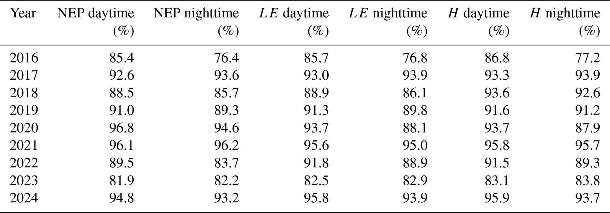
Following all quality control and filtering steps, substantial daytime and nighttime data coverage was retained for NEP, LE, and H throughout the study period (Table 1). Coverage was calculated separately for each year as the proportion of retained records among all daytime or nighttime half-hourly periods. Daytime and nighttime periods were defined as R_g>10 W m⁻² and R_g≤10 W m⁻², respectively. The reported percentages refer only to observed flux records.

Table 1 Annual coverage of retained high-quality half-hourly NEP, LE, and H records after quality control and filtering.

2.3.3 Gap-filling and uncertainty assessment

The removal of low-quality observations during quality control resulted in gaps in the half-hourly NEP, LE, and H records. These gaps were filled separately for each year using the extreme gradient boosting (XGBoost) algorithm. The predictors included air temperature, R_g, VPD, relative humidity, and sine and cosine transformations of day of year (DoY) to represent seasonal cyclicity. XGBoost was initially selected because it has previously been shown to reduce biases associated with marginal distribution sampling (MDS) at boreal EC sites (Vekuri et al., 2023). In the present study, model performance was evaluated by cross-validation and compared with MDS using the coefficient of determination (R²) and root mean square error (RMSE). The corresponding performance metrics are presented in Table B1. XGBoost generally produced similar or higher R² values and lower RMSE values than MDS, with the clearest improvements observed for LE and H, whereas performance differences for NEP were smaller and not consistent in every year. Based on its overall cross-validation performance across the three fluxes, XGBoost was selected as the final gap-filling method.

While air temperature and VPD were also included in the subsequent random forest (RF) driver analysis, gap-filling was performed at the half-hourly scale, whereas the driver analysis was based on daily RUEs calculated from aggregated fluxes. In addition, the response variables integrated several fluxes, rather than representing an individual gap-filled flux. This separation does not fully eliminate model-induced dependence, but it reduces the direct influence of individual gap-filled half-hourly records. The resulting relationships were therefore interpreted as ecosystem-scale associations rather than as fully independent causal effects.

To evaluate the gap-filling uncertainty, we conducted an artificial gap validation and Monte Carlo analysis. Gap-filling uncertainty was assessed separately for NEP and LE. In each validation run, 10 % of the measured half-hourly observations were temporarily removed, and XGBoost and MDS were used to fill the same artificial gaps. The differences between the observed and predicted values were then used as residuals. For each real missing half-hourly value, a residual obtained under similar meteorological and seasonal conditions was added to the corresponding gap-filled estimate, and this procedure was repeated in 1000 Monte Carlo realisations. The resulting annual distributions were used to derive 95 % uncertainty intervals representing gap-filling uncertainty only. Overall, the differences between the methods were small, although XGBoost generally produced slightly wider uncertainty intervals than MDS, particularly for NEP (Fig. C1).

2.3.4 Carbon flux partitioning

Carbon flux partitioning was used to separate NEP into GEP and R_eco:

$$\begin{array}{}\text{(1)}& \text{NEP}=\text{GEP}-R_{\text{eco}},\end{array}$$

where NEP represents the net ecosystem carbon balance, GEP is the total carbon uptake through photosynthesis, and R_eco is the total carbon flux from autotrophic and heterotrophic respiration. Following the ecological sign convention used throughout this study, positive NEP indicates net ecosystem carbon uptake, whereas negative NEP indicates net carbon release. GEP and R_eco are reported as positive fluxes.

GEP and R_eco were estimated using the nighttime partitioning approach of Reichstein et al. (2005), implemented in the REddyProc R package, version 1.3.4 (Wutzler et al., 2018). In this approach, R_eco is derived from the temperature response of measured nighttime NEP and subsequently extrapolated to daytime conditions. GEP is then calculated as the sum of NEP and R_eco.

The nighttime partitioning approach was selected to maintain methodological independence of GEP from radiation and VPD. Unlike daytime partitioning method, which parameterises GEP directly as a function of PAR and VPD (Lasslop et al., 2010), the nighttime approach avoids introducing these variables directly into the GEP estimates. This reduces the risk of built-in dependencies that could confound the subsequent analysis of environmental controls on RUEs.

2.3.5 Evapotranspiration calculation

Evapotranspiration was calculated from the quality controlled and gap-filled half-hourly LE series (Eq. 2):

$$\begin{array}{}\text{(2)}& \text{ET}={\displaystyle \frac{LE}{(\mathrm{2.501}-\mathrm{0.002361}\cdot T_{\text{air)}}\times {\mathrm{10}}^{\mathrm{6}}}},\end{array}$$

where ET is evapotranspiration ($\mathrm{kg}{\mathrm{H}}_{\mathrm{2}}\mathrm{O}{\mathrm{m}}^{-\mathrm{2}}{\mathrm{s}}^{-\mathrm{1}}$), LE is the latent heat flux (W m⁻²), 2.501 represents the latent heat of evaporation at 0 °C (MJ kg⁻¹), 0.002361 is the coefficient reflecting the reduction in energy required to evaporate 1 kg of water per degree Celsius increase ($\mathrm{MJ}{\mathrm{kg}}^{-\mathrm{1}}\mathrm{°}{\mathrm{C}}^{-\mathrm{1}}$), and T_air is the air temperature (°C) (Harrison, 1965). Evapotranspiration was not partitioned into transpiration and evaporation, as WUE was evaluated at the ecosystem scale to represent integrated carbon–water coupling rather than canopy-level processes.

2.3.6 Growing season determination

As direct phenological observations were unavailable for this site, the growing season was identified from the seasonal dynamics of daily GEP. The start of the season (SOS), peak of the season (POS), end of the season (EOS), and length of the season (LOS) were determined using the double-sigmoid model proposed by Gonsamo et al. (2013). The model described the observed seasonal GEP dynamics well, with R² values ranging from 0.88 to 0.93 across the study years (Fig. D1).

To test whether the choice of method affected the results, an alternative approach based on singular spectrum analysis (SSA) was applied. Daily GEP was smoothed using SSA, SOS and EOS were defined from threshold crossings that persisted for at least 5 d, using a threshold equal to 20 % of the annual maximum of smoothed GEP, and POS was defined as the day of maximum smoothed GEP. Both methods described the seasonal GEP dynamics similarly well, with R² values of 0.88–0.93 for the double-sigmoid model and 0.89–0.93 for SSA (Fig. D1).

The double-sigmoid model was retained as the main method because it describes the complete single-peaked seasonal GEP cycle, allows the spring increase and autumn decline to differ in shape and amplitude, and provides SOS, POS, and EOS directly from the fitted curve. Importantly, the method was specifically developed to avoid selecting a subjective GEP threshold (Gonsamo et al., 2013). In contrast, SSA smooths the daily GEP series but does not itself define the seasonal boundaries, which still depend on a user-selected threshold. In the absence of independent phenological observations, the SSA-derived dates cannot be considered more accurate solely because some appear more visually intuitive. The differences observed in 2020–2022 therefore represent method-specific operational definitions of the growing-season boundaries rather than evidence that either method identifies the true biological transition dates.

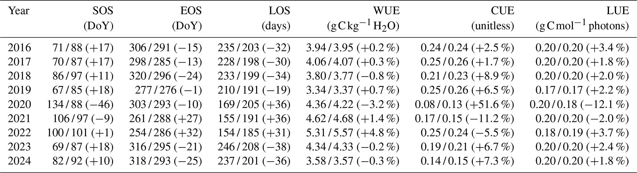
Compared with the double-sigmoid estimates, SSA-derived SOS ranged from 46 d earlier to 18 d later, EOS from 25 d earlier to 32 d later, and LOS from 38 d shorter to 36 d longer. Nevertheless, seasonal WUE and LUE estimates were generally similar between the methods, whereas CUE was more sensitive in some years (Table E1). Moreover, days with low GEP and, for WUE, low ET were excluded from the daily RUE analyses, reducing the influence of low-activity days near the seasonal boundaries (Sect. 2.3.7). Thus, the double-sigmoid model was retained as a consistent primary definition, while SSA was used as a sensitivity test of the growing-season determination.

2.3.7 Derivation of resource use efficiency metrics

RUEs were calculated at daily and growing-season scales from continuous gap-filled half-hourly data. Because these metrics are meaningful only during active vegetation, the analysis was restricted to the growing seasons. Daily GEP, NEP, ET, and PAR were obtained by summing half-hourly values, and growing-season totals were calculated by summing the corresponding daily values within each growing season. Daily WUE, CUE, and LUE were derived from daily flux totals, whereas growing-season efficiencies were calculated from the corresponding growing-season totals.

WUE was calculated as the ratio of GEP to ET, representing the trade-off between carbon gain and water loss (Eq. 3):

$$\begin{array}{}\text{(3)}& \text{WUE}={\displaystyle \frac{\text{GEP}}{\text{ET}}},\end{array}$$

where WUE is the water use efficiency (g C kg⁻¹ H₂O), GEP is the gross ecosystem production (g C m⁻² per period), and ET is the evapotranspiration (kg H₂O m⁻² per period). WUE quantifies how efficiently an ecosystem converts water loss into carbon uptake and serves as an indicator of ecosystem functioning and sensitivity to water availability and atmospheric drought. In this study, WUE represents integrated ecosystem-scale carbon-water coupling rather than leaf- or canopy-level physiological efficiency. Intrinsic WUE was not considered because canopy conductance and transpiration were not measured directly. Inherent WUE was also not used because it incorporates VPD into the efficiency metric, whereas VPD was analysed separately as an environmental driver. Rainfall and post-rainfall days were retained because the objective was to quantify ecosystem-scale WUE based on total ET, including both transpiration and wet-surfaces evaporation. Excluding these periods would selectively remove a component of ecosystem water loss and shift the interpretation toward a transpiration-based WUE metric.

Carbon use efficiency (CUE) was calculated as the ratio of NEP to GEP, expressing the fraction of carbon retained in the ecosystem after ecosystem respiration losses (Eq. 4):

$$\begin{array}{}\text{(4)}& \text{CUE}={\displaystyle \frac{\text{NEP}}{\text{GEP}}},\end{array}$$

where CUE is carbon use efficiency (unitless), NEP is net ecosystem production (g C m⁻² per period), and GEP is gross ecosystem production (g C m⁻² per period). CUE quantifies ecosystem-level carbon retention and reflects carbon sink strength, with higher CUE values indicating a greater fraction of assimilated carbon retained after ecosystem respiration losses.

Finally, LUE was calculated as the ratio of GEP to PAR, describing how efficiently the canopy converts light into carbon (Eq. 5):

$$\begin{array}{}\text{(5)}& \text{LUE}={\displaystyle \frac{\text{GEP}}{\text{PAR}}},\end{array}$$

where LUE is light use efficiency (g C mol⁻¹ photons), GEP is gross ecosystem production (g C m⁻² per period), and PAR is total photosynthetically active radiation (mol photons m⁻² per period). LUE characterizes ecosystem photosynthetic performance and reflects the efficiency of light utilization for carbon assimilation.

To ensure active ecosystem functioning, only days with GEP≥0.2 $\mathrm{g}\mathrm{C}{\mathrm{m}}^{-\mathrm{2}}{\mathrm{d}}^{-\mathrm{1}}$ were included. For WUE, an additional criterion of ET≥0.2 $\mathrm{kg}{\mathrm{H}}_{\mathrm{2}}\mathrm{O}{\mathrm{m}}^{-\mathrm{2}}{\mathrm{d}}^{-\mathrm{1}}$ was applied to ensure the inclusion of days with meaningful water fluxes. In the case of CUE and LUE, only the GEP threshold was used. RUEs outliers were identified using the interquartile range (IQR) method. Observations falling outside the range from ${\text{Q}}_{\mathrm{1}}-\mathrm{1.5}\times \text{IQR}$ to ${\text{Q}}_{\mathrm{3}}+\mathrm{1.5}\times \text{IQR}$ were excluded from the analysis.

2.4 Statistical data analysis

Statistical trends across the 2016–2024 growing seasons were tested using ordinary least squares (OLS) regression. Residual autocorrelation in the OLS regression residuals was assessed using Durbin–Watson tests, and the robustness of trend significance was evaluated using Newey–West standard errors.

Growing seasons with atypical meteorological conditions or RUEs were identified using a leave-one-year-out approach. For each growing season, day-of-year medians were calculated from all remaining years, and daily anomalies were defined as deviations from these reference medians. The anomalies were evaluated using a one-sample Wilcoxon signed-rank test. A growing season was classified as anomalous only when its seasonal summary metric differed by more than ±20 % from the multi-year median and the distribution of daily anomalies differed significantly from zero (p<0.05). The 20 % threshold was applied as a pragmatic effect-size filter to distinguish functionally relevant shifts among growing seasons from minor ecological fluctuations.

To determine the main environmental drivers of daily RUEs, a complementary two-step approach was used. First, the relative importance of each driver (air temperature, soil temperature, ET, PAR, precipitation, SWC₁₀, and VPD) was evaluated using the RF algorithm implemented in the randomForest package in R (Liaw and Wiener, 2002). The analysis was repeated 1000 times, with 70 % of the data used for model training and the remaining 30 % for validation. Predictor importance was quantified using the percentage increase in mean squared error (%IncMSE). This metric describes how much the model prediction error increases when the values of a predictor are randomly rearranged. Higher %IncMSE values indicate greater predictor importance.

Second, single-driver generalized additive models (GAMs) were applied to examine how each RUE varied along individual environmental gradients and to characterize potential nonlinear response patterns. The GAMs were fitted to the complete dataset using the mgcv package in R (Wood, 2003, 2011; Wood et al., 2016). To reduce the influence of sparsely sampled extreme predictor values on interpretation, the fitted response curves were evaluated primarily within the 5th–95th percentile range of each environmental driver. These percentile limits were used only to define the central range for visualization and interpretation and did not affect model fitting. R² values were calculated for each fitted model. Thus, RF was used to rank the overall predictive importance of the variables, whereas GAMs were used to describe the form of their individual relationships with RUEs.

To assess the variability of RUEs under different hydrometeorological conditions, we used the Standardized Precipitation-Evapotranspiration Index (SPEI), calculated for 2016–2024 with the SPEI package in R (Beguería and Vicente-Serrano, 2023). SPEI was selected because it integrates both precipitation and atmospheric evaporative demand and is therefore well suited for assessing ecosystem-scale responses of RUEs to hydrometeorological variability. The input time series was derived from the water balance, defined as the difference between precipitation and potential ET, the latter estimated using the Penman equation (Penman, 1948). A three-month accumulation timescale was used, meaning that each monthly SPEI value represented the cumulative climatic water balance of that month and the preceding two months. SPEI-3 is widely used to characterize seasonal drought and ecosystem responses because it captures persistent moisture conditions while reducing the influence of short-term fluctuations (Huang and Zhai, 2024; Vicente-Serrano et al., 2010). Hydrometeorological conditions were classified according to established SPEI categories: “Extremely wet” (SPEI≥2), “Severely wet” ($\mathrm{1.5}\le \text{SPEI}<\mathrm{2}$), “Moderately wet” ($\mathrm{1}\le \text{SPEI}<\mathrm{1.5}$), “Mildly wet” ($\mathrm{0.5}\le \text{SPEI}<\mathrm{1}$), “Normal” ($-\mathrm{0.5}<\text{SPEI}\le \mathrm{0.5}$), “Mild drought” ($-\mathrm{1}<\text{SPEI}\le -\mathrm{0.5}$), “Moderate drought” ($-\mathrm{1.5}<\text{SPEI}\le -\mathrm{1}$), “Severe drought” ($-\mathrm{2}<\text{SPEI}\le -\mathrm{1.5}$) and “extreme drought” ($\text{SPEI}\le -\mathrm{2}$) (Vicente-Serrano et al., 2010). Monthly SPEI values were assigned to each day within the corresponding month, and daily RUE metrics were grouped by SPEI class. As an independent robustness check, SPEI-3 was recalculated using the longer Tartu–Tõravere meteorological record (2004–2024). The resulting values were strongly correlated with the original Soontaga SPEI-3 (r=0.83), while SPEI-3 calculated for Tartu–Tõravere using 9- and 21-year reference periods was nearly identical (r=0.98), indicating that the shorter reference period had little influence on the overall hydrometeorological patterns (Fig. F1).

Normality of WUE and CUE distributions was evaluated using the Shapiro–Wilk test. Since the data did not meet the assumption of normality, nonparametric comparisons were applied. To assess the effect of hydrological stress, each SPEI category was statistically compared against the “Normal” group using pairwise Wilcoxon rank-sum (Mann-Whitney) tests with Bonferroni correction for multiple comparisons.

Because PAR, the denominator of LUE, exhibits a pronounced seasonal cycle determined by solar geometry, day length, and cloud conditions, raw comparisons of LUE among SPEI classes may be influenced by the unequal distribution of these classes across the growing season. This issue is specific to LUE because PAR represents an external radiative forcing rather than an ecosystem flux response. An additional seasonality-adjusted analysis was performed to distinguish changes in carbon uptake relative to the radiation expected for the same time of year from differences caused by the seasonal composition of the SPEI classes. For each observation, leave-one-year-out reference values of GEP and PAR were calculated as day-of-year medians within a ±7 d moving window. The seasonally adjusted LUE log deviation was calculated as Eq. (6):

$$\begin{array}{}\text{(6)}& {\text{LUE}}_{\text{anom}}=\log \left({\displaystyle \frac{\text{GEP}}{{\text{GEP}}_{\text{ref}}}}\right)-\log \left({\displaystyle \frac{\text{PAR}}{{\text{PAR}}_{\text{ref}}}}\right)\end{array}$$

where GEP_ref and PAR_ref are the leave-one-year-out median GEP and PAR values calculated for the corresponding day of year using a ±7 d moving window. LUE_anom represents the deviation of daily LUE from its seasonally expected value. For each SPEI class, the median LUE_anom was calculated and expressed as the difference from the median of the normal class. The GEP and PAR components were treated in the same way to determine whether differences in adjusted LUE were associated primarily with deviations in carbon uptake or radiation availability. Uncertainty in the class differences was quantified using 2000-year-level cluster-bootstrap resamples, in which complete years were sampled with replacement. A class difference was considered statistically supported when its 95 % bootstrap confidence interval did not include zero.

All calculations were performed using R software (R Core Team, 2024), version 4.3.3.

3 Results

3.1 Growing-season dynamics of environmental drivers and seasonal metrics

Over the nine-year period, the median LOS was 228 d. The median SOS occurred on 23 March (DoY 82), while the median POS and EOS were observed on 16 July (DoY 197) and 30 October (DoY 303), respectively (Table 2).

Table 2 Growing seasons metrics by year.

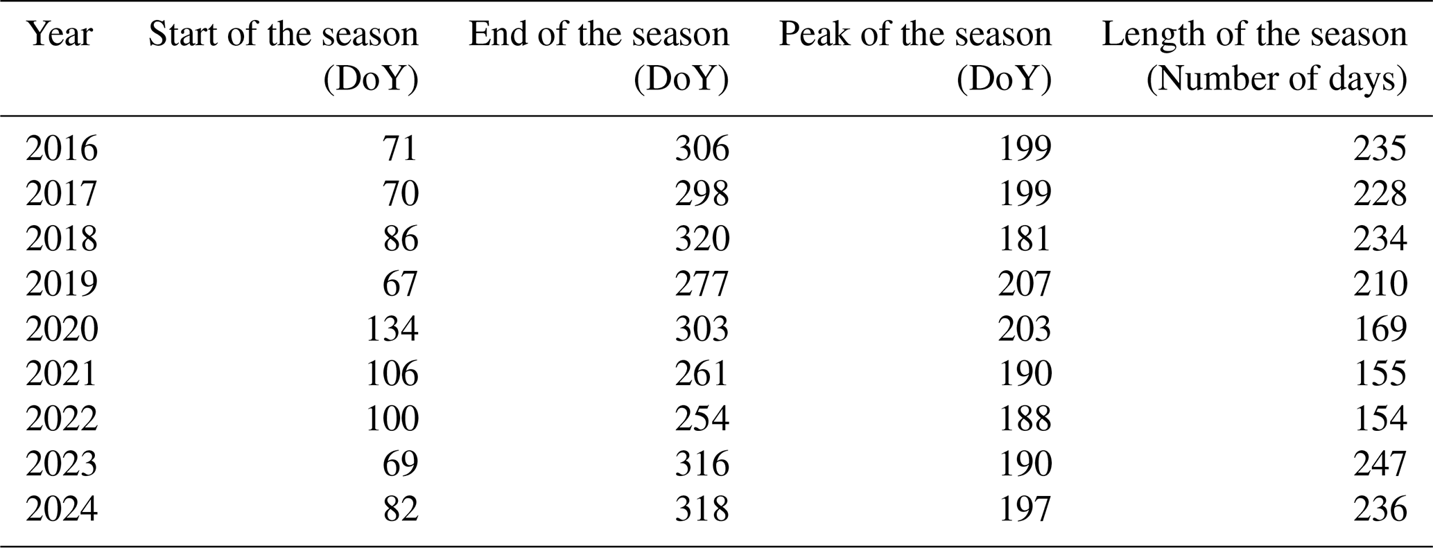
During 2020, 2021, and 2022, the LOS was substantially shorter than the median value for the whole study period (−26 %, −32 %, and −33 %, respectively). In 2020, this reduction was primarily due to a late start of the growing season on 13 May, while the end date on 29 October aligned with the 9-year median. In contrast, the 2021 growing season began on 16 April and ended earlier than the median, on 18 September, resulting in a shorter season. A similar pattern was observed in 2022, with the season starting on 10 April and ending prematurely on 11 September. Despite these shifts in the timing and duration of the growing season, the timing of the POS remained stable.

Over the 2016–2024 period, significant increasing trends (p<0.05) were observed for median seasonal air temperature and median seasonal VPD (Fig. 2a and c). No significant residual autocorrelation was detected for the air temperature and VPD trend models using the Durbin–Watson test (p=0.47 and 0.43, respectively), and both trends remained significant when evaluated using Newey–West standard errors (p=0.019 and 0.031, respectively).

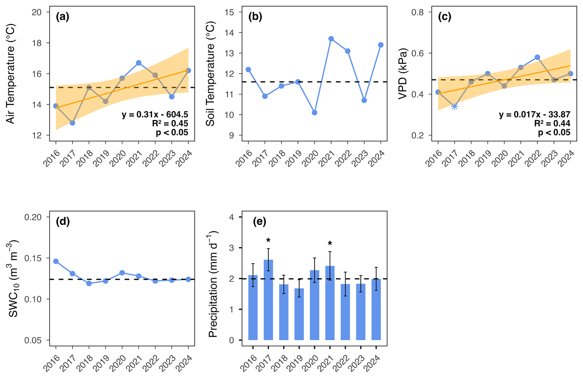
Figure 2 Variation in growing-season environmental drivers from 2016 to 2024: (a) median seasonal air temperature, (b) median seasonal soil temperature, (c) median seasonal vapour pressure deficit (VPD), (d) median seasonal soil water content at 10 cm depth (SWC₁₀), and (e) mean daily precipitation. Blue points and bars represent seasonal or daily values, dashed black lines indicate 9-season medians, and orange lines show significant linear trends (p<0.05). Shaded areas represent standard errors, and asterisks indicate anomalous growing seasons that met anomaly criteria.

Median growing-season VPD was classified as anomalously low only in 2017, when it fell 28 % below the multi-year median. Although VPD in 2022 was 23 % above the multi-year median and exceeded the effect-size threshold, it was not statistically significant and was therefore not classified as anomalous. Mean daily precipitation was anomalously high in 2017 and 2021, exceeding the multi-year median by 31 % and 21 %, respectively. No other growing seasons met both the effect-size and statistical-significance criteria.

3.2 Growing-season variation in water, carbon, and light fluxes and resource use efficiencies

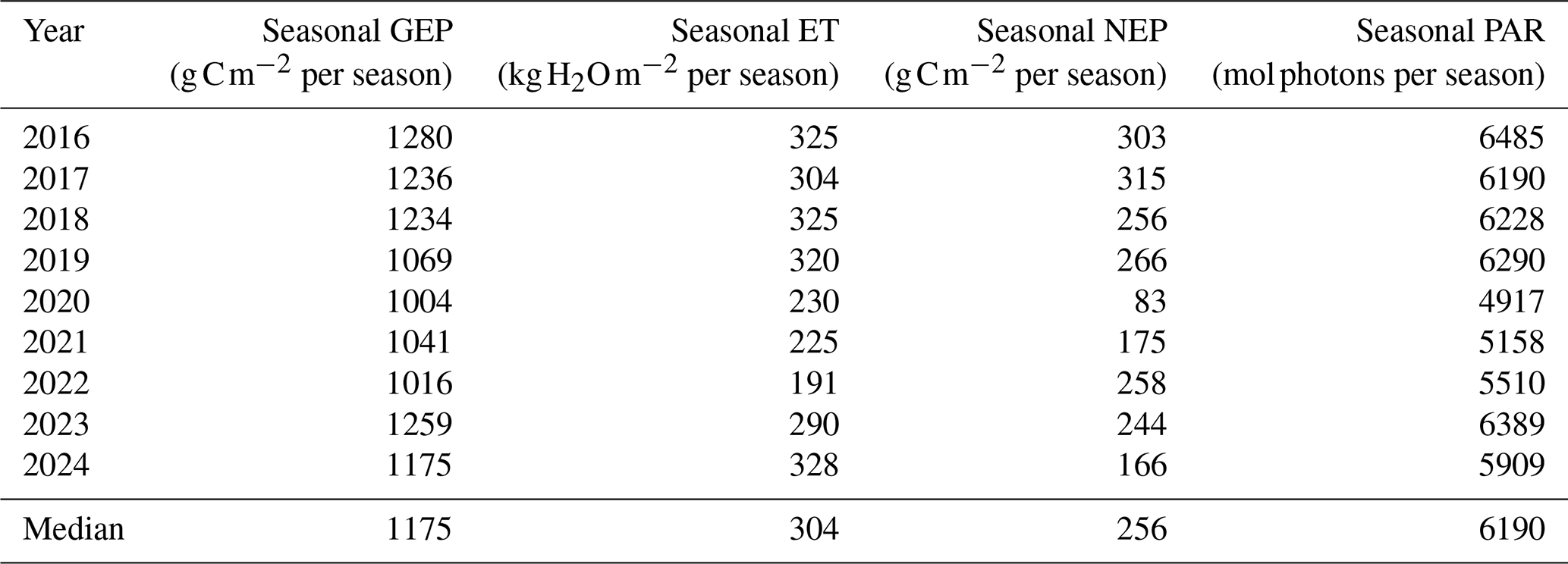
Over the 2016–2024 period, no statistically significant trends were detected in growing-season totals or mean daily values of ET, GEP, NEP, or PAR (Table 3). Based on the predefined anomaly criteria, growing-season ET was 24 %, 26 %, and 37 % lower than the multi-year median of 304 kg H₂O m⁻² per season in 2020, 2021, and 2022, respectively. Growing-season NEP was 23 % higher than its multi-year median of 256 g C m⁻² per season in 2017, but 68 %, 32 %, and 35 % lower in 2020, 2021, and 2024, respectively. No anomalous growing-season values were detected for GEP or PAR.

Table 3 Growing season totals of GEP, NEP, ET, and PAR.

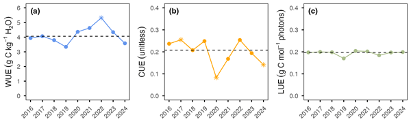
RUEs varied among growing seasons without a common pattern, and none exhibited a significant temporal trend across the nine study years (Fig. 3).

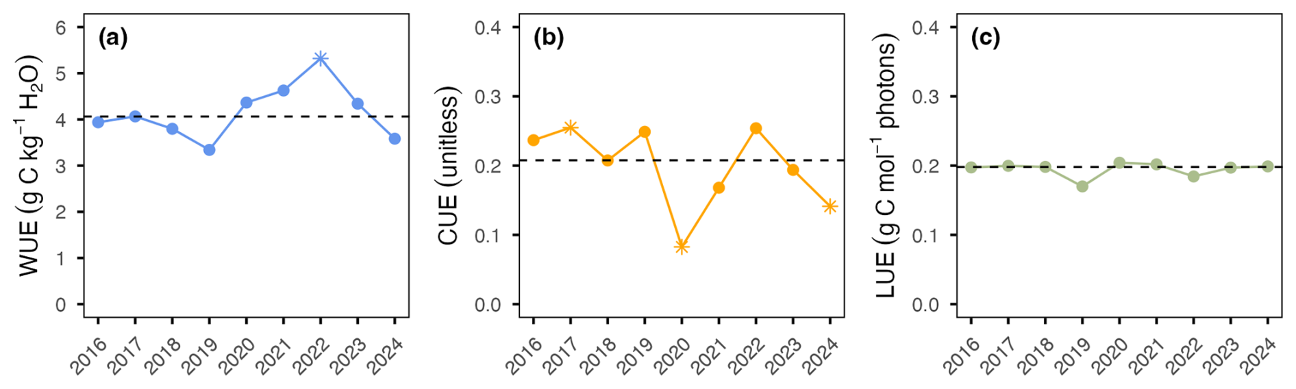
Figure 3 Growing-season dynamics of resource use efficiencies from 2016 to 2024: (a) water use efficiency (WUE), (b) carbon use efficiency (CUE), and (c) light use efficiency (LUE). Blue, orange, and green points represent growing-season values. Dashed black lines indicate the nine-year median for each parameter. Asterisks indicate growing seasons that met anomaly criteria.

Based on the predefined criteria, WUE was classified as anomalously high only in 2022, exceeding the multi-seasonal median of 4.1 g C kg⁻¹ H₂O by 23 %. In 2019, WUE was significantly lower than the multi-seasonal median (3.34 vs. 4.06 g C kg⁻¹ H₂O; −17.7 %, p<0.05), but the deviation did not exceed the 20 % effect-size threshold and therefore did not meet the anomaly criteria. CUE was 23 % above its multi-year median of 0.21 in 2017 and 60 % and 32 % below it in 2020 and 2024, respectively, with all three growing seasons classified as anomalous. No anomalous growing-season values were detected for LUE.

3.3 Influence of environmental drivers on resource use efficiencies

The RF models based on daily values achieved moderate predictive accuracy for WUE (R²=0.21), whereas they explained a substantially greater proportion of the observed variance for CUE (R²=0.59) and LUE (R²=0.60) (Fig. 4).

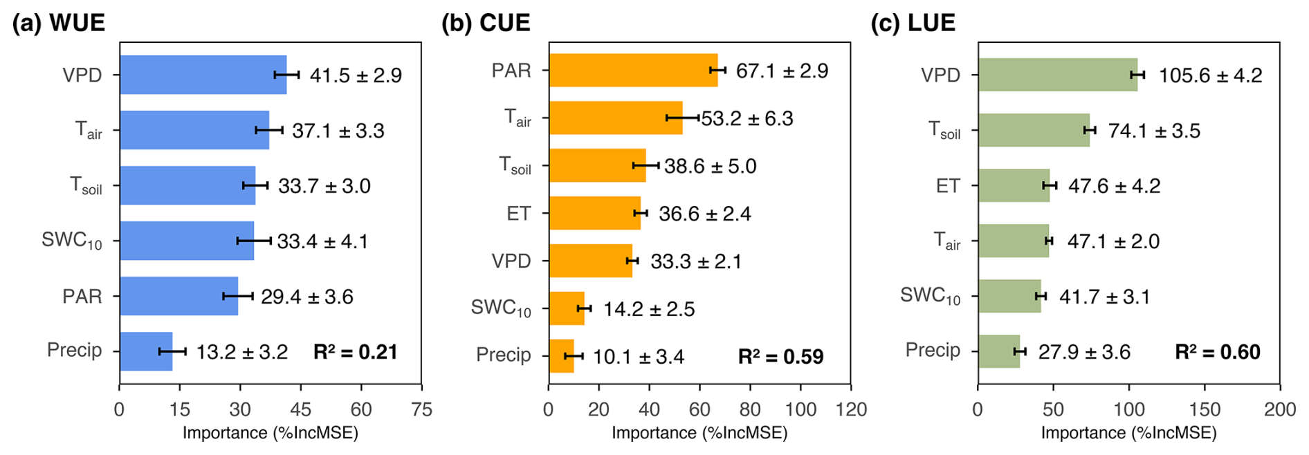
Figure 4 Relative importance of daily environmental drivers of resource use efficiencies derived from random forest models: (a) water use efficiency (WUE), (b) carbon use efficiency (CUE), and (c) light use efficiency (LUE). Predictors are photosynthetically active radiation (PAR), vapour pressure deficit (VPD), evapotranspiration (ET), air temperature (T_air), soil temperature at 10 cm depth (T_soil), soil water content at 10 cm depth (SWC₁₀), and precipitation (Precip). Reported R² values indicate the proportion of variance explained by each model.

The predictor importance analysis revealed distinct patterns among the RUEs. For daily WUE, VPD emerged as the strongest driver, followed by air temperature. In the case of daily CUE, PAR was the most important predictor, with air temperature again ranking second. For daily LUE, VPD showed the highest influence, followed by soil temperature. Notably, precipitation consistently exhibited very low importance across all models, emphasizing its limited role in explaining daily variability of RUEs.

For WUE, individual GAMs explained 2 %–10 % of the variance, with the strongest relationships observed for PAR, VPD, and air temperature. Given that the multivariate RF model explained only 21 % of daily WUE variability (Fig. 4), the comparatively modest R² values of the univariate GAMs should not be interpreted as evidence of poor model performance; rather, they indicate that individual drivers account for a meaningful share of the overall predictability captured by the RF model. For CUE, individual GAMs explained 2 %–38 % of the variance, with PAR accounting for the largest proportion. For LUE, individual GAMs explained 1 %–20 % of the variance, with the strongest relationships observed for soil and air temperature (Fig. 5).

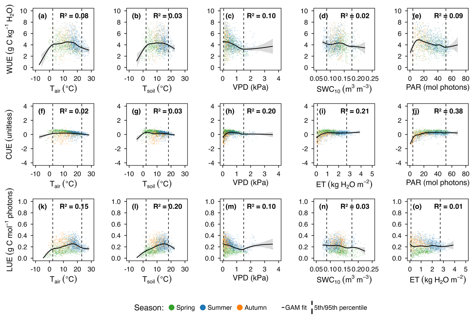
Figure 5 Generalized additive model relationships between daily environmental drivers and resource use efficiencies: (a–e) water use efficiency (WUE), (f–j) carbon use efficiency (CUE), and (k–o) light use efficiency (LUE). Environmental drivers are air temperature (T_air), soil temperature at 10 cm depth (T_soil), vapour pressure deficit (VPD), soil water content at 10 cm depth (SWC₁₀), evapotranspiration (ET), and photosynthetically active radiation (PAR). Points show daily values coloured by season (spring, summer, autumn). Solid black lines show GAM fits with 95 % confidence intervals (grey shading), and dashed vertical lines indicate the 5th and 95th percentiles of the observed predictor distributions. Reported R² values indicate the proportion of variance explained by each model.

To reduce the influence of sparsely sampled extremes, the GAM response shapes were interpreted within the 5th–95th percentile range of each environmental driver, although the models were fitted using the complete dataset. Within this range, WUE generally decreased with increasing VPD. WUE increased at low temperatures, remained relatively stable at intermediate temperatures, and decreased at higher temperatures. WUE also increased at low PAR and then gradually declined as PAR increased. CUE showed its clearest response to PAR, increasing rapidly at low irradiance and approaching a plateau at moderate to high PAR. LUE generally decreased with increasing VPD and showed hump-shaped relationships with both air and soil temperature, increasing from low to intermediate temperatures and decreasing at higher temperatures.

3.4 SPEI dynamics and influence on resource use efficiencies

Among the 1732 growing-season days included in the SPEI analysis, 153 (8.8 %) were classified as severe drought, 168 (9.7 %) as moderate drought, 193 (11.1 %) as mild drought, 674 (38.9 %) as normal, 213 (12.3 %) as mildly wet, 184 (10.6 %) as moderately wet, and 147 (8.5 %) as severely wet.

Daily WUE was generally stable across SPEI classes, with a modest but statistically significant reduction under moderate drought (3.7 g C kg⁻¹ H₂O, −10 %, p<0.05) (Fig. 6a). This reduction coincided with a proportionally larger increase in ET than in GEP relative to normal conditions (1.6 vs. 1.4 $\mathrm{kg}{\mathrm{H}}_{\mathrm{2}}\mathrm{O}{\mathrm{m}}^{-\mathrm{2}}{\mathrm{d}}^{-\mathrm{1}}$, +14 %; and 5.9 vs. 5.7 $\mathrm{g}\mathrm{C}{\mathrm{m}}^{-\mathrm{2}}{\mathrm{d}}^{-\mathrm{1}}$, +4 %, respectively) (Table F1).

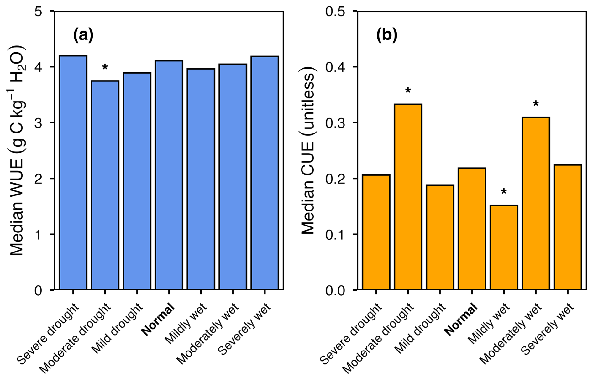
Figure 6 Median daily resource use efficiencies across hydrometeorological gradient defined by the Standardized Precipitation–Evapotranspiration Index: (a) water-use efficiency (WUE), and (b) carbon use efficiency (CUE). The normal class ($-\mathrm{0.5}<\text{SPEI}\le \mathrm{0.5}$) was used as the statistical reference. Asterisks denote statistically significant differences from the normal class (pairwise Wilcoxon rank-sum tests with Bonferroni correction; p<0.05). SPEI categories span severe drought to severely wet conditions: severely wet ($\mathrm{1.5}\le \text{SPEI}<\mathrm{2}$), moderately wet ($\mathrm{1}\le \text{SPEI}<\mathrm{1.5}$), mildly wet ($\mathrm{0.5}\le \text{SPEI}<\mathrm{1}$), mild drought ($-\mathrm{1}<\text{SPEI}\le -\mathrm{0.5}$), moderate drought ($-\mathrm{1.5}<\text{SPEI}\le -\mathrm{1}$), and severe drought ($-\mathrm{2}<\text{SPEI}\le -\mathrm{1.5}$) (Vicente-Serrano et al., 2010).

For CUE, significant increases were detected under moderate drought (0.33, +50 %, p<0.05) and moderately wet conditions (0.31, +41 %, p<0.05), whereas a significant reduction occurred under mildly wet conditions (0.15, −32 %, p<0.05) (Fig. 6b). Under moderate drought, the increase in daily CUE coincided with a substantially larger increase in NEP than in GEP relative to normal conditions (1.7 vs. 1.2 $\mathrm{g}\mathrm{C}{\mathrm{m}}^{-\mathrm{2}}{\mathrm{d}}^{-\mathrm{1}}$, +42 %; and 5.9 vs. 5.7 $\mathrm{g}\mathrm{C}{\mathrm{m}}^{-\mathrm{2}}{\mathrm{d}}^{-\mathrm{1}}$, +4 %, respectively), while R_eco decreased (4.5 vs. 4.9 $\mathrm{g}\mathrm{C}{\mathrm{m}}^{-\mathrm{2}}{\mathrm{d}}^{-\mathrm{1}}$, −8 %) (Table F1). A similar pattern occurred under moderately wet conditions, where NEP increased more strongly than GEP (1.8 vs. 1.2 $\mathrm{g}\mathrm{C}{\mathrm{m}}^{-\mathrm{2}}{\mathrm{d}}^{-\mathrm{1}}$, +50 %; and 6.4 vs. 5.7 $\mathrm{g}\mathrm{C}{\mathrm{m}}^{-\mathrm{2}}{\mathrm{d}}^{-\mathrm{1}}$, +12 %, respectively), accompanied by a slight decline in R_eco (4.6 vs. 4.9 $\mathrm{g}\mathrm{C}{\mathrm{m}}^{-\mathrm{2}}{\mathrm{d}}^{-\mathrm{1}}$, −6 %) (Table F1). By contrast, under mildly wet conditions, the strong increase in GEP was nearly matched by an increase in R_eco (7.6 vs. 5.7 $\mathrm{g}\mathrm{C}{\mathrm{m}}^{-\mathrm{2}}{\mathrm{d}}^{-\mathrm{1}}$, +33 %; and 6.6 vs. 4.9 $\mathrm{g}\mathrm{C}{\mathrm{m}}^{-\mathrm{2}}{\mathrm{d}}^{-\mathrm{1}}$, +35 %, respectively), resulting in a change in NEP (1.1 vs. 1.2 $\mathrm{g}\mathrm{C}{\mathrm{m}}^{-\mathrm{2}}{\mathrm{d}}^{-\mathrm{1}}$, −8 %) and a lower CUE (Table F1).

Seasonally adjusted daily LUE remained relatively stable across most SPEI classes, with a statistically supported departure from the Normal class observed only under severely wet conditions (Fig. 7a). Under these conditions, adjusted LUE was significantly higher (+13.9 %, 95 % CI: +2.6 % to +31.4 %), reflecting a stronger decline in PAR (−11.6 %) than in GEP (−1.3 %) relative to Normal conditions (Fig. 7b). Mild drought showed the largest negative point estimate (−14.5 %, 95 % CI: −24.5 % to +11.7 %), but its broad bootstrap confidence interval included zero. No consistent differences from the Normal class were detected for the remaining SPEI classes.

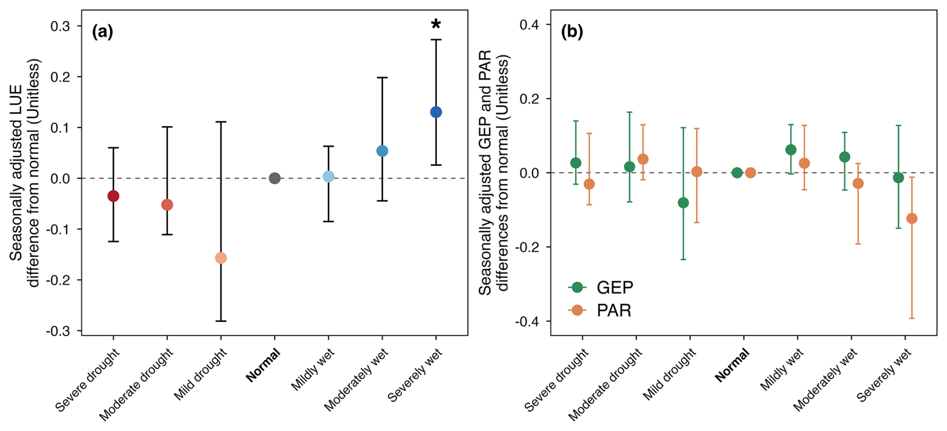
Figure 7 Seasonally adjusted differences in daily light use efficiency (LUE) and its gross ecosystem production (GEP) and photosynthetically active radiation (PAR) components across SPEI classes: (a) LUE differences and (b) GEP and PAR differences relative to the normal class. Points represent median differences expressed as natural-log ratios, and error bars indicate 95 % confidence intervals obtained from 2000-year-level cluster-bootstrap resamples. The dashed horizontal line indicates no difference from the normal class, and the asterisk denotes a 95 % bootstrap confidence interval that does not include zero.

4 Discussion

4.1 Positive trends in air temperature and vapour pressure deficit

Our study revealed increasing air temperature and VPD during nine growing seasons (Fig. 2a and c). This finding aligns with global observations showing widespread increases in both air temperature and VPD driven by ongoing climate warming (Fang et al., 2022; IPCC, 2023; Shekhar et al., 2024; Vickers and Mahrt, 1997). Similar trends have been documented in boreal forest ecosystems across the Northern Hemisphere. For example, Siberian boreal forests have experienced persistent increases in air temperature and VPD since the 1980s (Zharkov et al., 2021) and similar long-term increases in VPD associated with rising air temperature have been documented across Canadian boreal forests (Mirabel et al., 2023). In the region closest to our study site, long-term observations from Finland show an increase in growing degree days (GDD, which represents the cumulative sum of daily mean temperatures exceeding a base threshold for plant growth) especially in the southern part of boreal zone (Kauppi et al., 2014).

These ongoing shifts in atmospheric conditions carry important consequences for forest functioning. Increasing VPD has been linked to reduced vegetation growth (Restaino et al., 2016; Vickers and Mahrt, 1997) and higher forest mortality rates (Williams et al., 2013). In the boreal zone, rising VPD is associated with declining growth of coniferous species (Laudon et al., 2024; Mirabel et al., 2023), while rising temperatures not only limit coniferous species productivity but also promote the expansion of broad-leaved trees (Fu et al., 2023), leading to shifts in stand composition. Moreover, changes in temperature and VPD are increasing the frequency of droughts (Hammond et al., 2022), wildfire risks (Clarke et al., 2022; Luo et al., 2025), and pest outbreaks (Venäläinen et al., 2020), further elevating tree mortality.

While we did not observe increased tree mortality, wildfires, or pest outbreaks during the study period, such disturbances may still occur under continued climatic change. The transitional position of the hemiboreal zone makes its forest ecosystems particularly vulnerable to climate change. If current trends of rising VPD and air temperature continue, large-scale biogeographic shifts in hemiboreal forests are possible (Toot et al., 2020).

4.2 Resource use efficiency patterns across growing seasons

4.2.1 WUE stability across growing seasons

The WUE observed in our study (3.3–5.3 g C kg⁻¹ H₂O) aligns well with various mature boreal and temperate coniferous forests. For example, a 130-year-old boreal stand in Saskatchewan, Canada, exhibited a WUE of 3.1 g C kg⁻¹ H₂O (Beer et al., 2009; Krishnan et al., 2008). In a 100-year-old coniferous forest in Howland, USA, WUE reached 4.0 g C kg⁻¹ H₂O (Beer et al., 2009; Hollinger et al., 1999), while a temperate pine forest of similar age in Loobos, the Netherlands had a WUE of 3.8 g C kg⁻¹ H₂O (Beer et al., 2009; Dolman et al., 2002). Recently, Krasnova et al. (2026) reported multiyear average WUE values of 3.5 ± 0.4 and 4.2 ± 0.3 g C kg⁻¹ H₂O for mature mixed spruce–pine and pure pine forests, respectively, in northern Sweden. These values fall within the range observed in our study and further support the consistency of our WUE estimates.

At our study site, WUE remained relatively stable across the nine growing seasons despite substantial variability in environmental conditions, with only 2022 meeting the predefined anomaly criteria (Fig. 3a). In that year, the shortest growing season (Table 2) limited ecosystem activity to a brief period, during which carbon uptake through photosynthesis was maintained relatively well (1016 g C m⁻² per season, 14 % below the multi-year median), whereas total ET was strongly reduced (191 kg H₂O m⁻² per season, 37 % below the multi-year median) (Table 3). The relatively well-maintained seasonal GEP indicates efficient photosynthetic functioning during active days, while ET remained constrained because the season was short and lacked long episodes of high atmospheric demand (high VPD) and persistently optimal radiation (Fig. G1). Thus, stomatal regulation likely maintained carbon gain during favourable windows while limiting cumulative water loss, leading to a decoupling of GEP from ET at the seasonal scale and resulting in anomalously high WUE. Taken together, this pattern points to stomatal regulation as a key mechanism buffering WUE across seasons by maintaining carbon gain during short favourable periods while limiting cumulative water loss. When the growing season is short and high atmospheric demand is rare, this regulation can suppress ET more strongly than GEP, producing unusually high annual WUE as observed in 2022. However, this interpretation should be treated with caution because the seasonal EBR was lowest in 2022 (Table H1), which can lead to underestimation of turbulent fluxes, particularly ET, and thus propagate into the WUE estimate.

The observed WUE stability suggests a strong physiological regulation of coniferous forests, with a consistent balance between carbon gain and water loss (Jiang et al., 2022; Kuglitsch et al., 2008). This interpretation is further supported by the dominant influence of VPD and the negligible importance of precipitation in our analysis (Fig. 4a), as well as by measurements in a comparable boreal pine-spruce forest, where transpiration accounted for 65 % of growing-season ET, compared with 20 % from interception evaporation and 15 % from forest-floor evaporation (Grelle et al., 1997). Nevertheless, because WUE was calculated using total ET, interception evaporation may also have contributed to its variability. Furthermore, several studies indicate that WUE stability is often supported by moderate precipitation and the maintenance of optimal soil moisture, which together enhance carbon uptake while limiting evaporative losses (Keenan et al., 2013; Montibeller et al., 2022; Xu et al., 2023). In line with this mechanism, SWC₁₀ at our site remained highly stable across years, even as precipitation varied (Fig. 2d and e). However, SWC₁₀ was measured only in the upper soil layer (10 cm), which may be of limited relevance in sandy soils with high infiltration and deep drainage. Overall, our findings indicate that the observed WUE stability reflects the current capacity of hemiboreal coniferous forests to maintain a long-term water–carbon balance under variable conditions. However, continued warming and increasing VPD could alter this pattern in the future.

4.2.2 Growing-season CUE variability and temperature control

In our study, CUE ranged from 0.08 to 0.25, which is slightly lower than the values reported for boreal and temperate coniferous forests. For example, a 150-year-old black spruce (Picea mariana) stand in Canada exhibited CUE values between 0.17 and 0.20 (Ryan et al., 1997). For a 110–118-year-old temperate Norway spruce forest at the Tharandt Anchor Station in Germany, we calculated annual CUE values ranging from 0.24 to 0.33 using NEP and GPP measurements (Grünwald and Bernhofer, 2007). For a nearby boreal site in southern Finland dominated by ∼55-year-old Scots pine, we calculated a mean growing-season (May–September) CUE of 0.32 ± 0.04 for the period 2001–2017 based on long-term EC data (Launiainen et al., 2022). Differences across studies may be explained by a combination of site-specific factors including environmental conditions, forest structure, and stand age (Collalti et al., 2020; West, 2020). The relatively low values observed at our site indicate that a substantial portion of carbon fixed by photosynthesis is returned to the atmosphere through respiration, emphasizing the strong influence of soil and plant respiration on net carbon balance. In this context, CUE provides an integrated measure of ecosystem-level carbon retention rather than plant-level growth efficiency, highlighting the importance of considering both productivity and respiration when assessing the carbon sink strength of hemiboreal forests.

In a previous study at this site, we found that ecosystem NEP was mainly controlled by R_eco, which in turn was closely linked to air temperature (Rogozin et al., 2026). The current study supports this previously observed relationship, as seasonal NEP declined with increasing growing-season air temperature (Fig. I1). This temperature dependence was particularly relevant to the CUE anomalies observed in 2017 and 2024. In 2017, high seasonal NEP and elevated CUE were observed during the coldest growing season of the study period, whereas in 2024, low NEP and reduced CUE occurred under comparatively warm conditions (Fig. I1). In 2020, NEP was low due to a combination of factors, including an anomalous June and an unusually warm autumn, which are described in detail in Rogozin et al. (2026). These results support the idea that air temperature is a key factor regulating seasonal NEP and thus seasonal CUE.

4.2.3 Growing-season LUE stability and potential canopy controls

The remarkable stability of LUE across all nine growing seasons (0.17–0.20 g C mol⁻¹ photons; Fig. 3c) places our values within the range reported for boreal and temperate coniferous ecosystems. A ∼100-year-old mixed Scots pine–Norway spruce stand in Sweden showed LUE of ∼0.12–0.15 g C mol⁻¹ photons (originally 0.57–0.71 g C MJ⁻¹), with variability largely explained by daytime air temperature (Lagergren et al., 2005). An upland red pine (Pinus resinosa) plantation in Wisconsin (∼90–120 years) exhibited growing-season LUE of ∼0.21–0.23 g C mol⁻¹ photons (originally 0.46 ± 0.08 g C MJ⁻¹ in 1999 and 0.50 ± 0.09 g C MJ⁻¹ in 2000), with an interannual increase attributed to post-drought recovery (Ahl et al., 2004). Interestingly, the stand closest to our site, a ∼55-year-old Scots pine stand in southern Finland, had a 17-year mean LUE of 0.21 ± 0.02 g C mol⁻¹ photons (originally 17.83 ± 1.63 mmol mol⁻¹) (Launiainen et al., 2022), similar to our values despite a substantial age difference. This convergence across stands challenges the assumption that LUE invariably declines with stand maturation (Ryan et al., 1997; Xu et al., 2020). At our site, this implies that long-term carbon uptake may be constrained more by the amount and timing of available light (and associated seasonality) than by any progressive decline in photosynthetic efficiency with stand age.

The observed low variation in growing-season LUE across years likely reflects the combined stability of both seasonal PAR and GEP, each varying by <20 % across years, consistent with relatively constant light environment and previously demonstrated low GEP variability of our forest (Rogozin et al., 2026). In old conifer stands, crown level traits including shoot scale clumping and needle angle distributions optimise within canopy light capture and reduce self-shading, thereby sustaining LUE despite aging (Kim et al., 2011; Ollinger, 2011; Stenberg, 1996). The persistently stable LUE observed in our site likely reflects a structurally stable canopy that maintains efficient light partitioning from year to year. We acknowledge that the absence of direct measurements of foliage structure and biomass constrains mechanistic attribution. Nevertheless, our results demonstrate that old-growth forest can maintain stable LUE, providing a basis for future work on long-term photosynthetic dynamics in aging hemiboreal ecosystems.

4.3 Environmental regulation of daily resource use efficiencies

4.3.1 Atmospheric dryness constrains WUE and LUE

VPD emerged as the highest-ranked driver of daily WUE and LUE (Fig. 4a and c), with both efficiencies generally declining as atmospheric dryness increased (Fig. 5c and m). This response likely reflects progressive stomatal closure that reduces canopy conductance and CO₂ uptake under higher evaporative demand (Jarvis, 1976; Lange et al., 1971). Because WUE is based on total ecosystem ET, enhanced soil evaporation at high VPD can further lower apparent carbon gain per unit water loss (Tang et al., 2014). Similar VPD-driven declines in daily WUE and LUE have been reported in boreal and temperate coniferous forests (Gao et al., 2017; Krasnova et al., 2026; Zhang et al., 2015) and are consistent with broader increases in atmospheric dryness (Novick et al., 2024). Taken together, these results identify atmospheric dryness as an important first-order short-term constraint on carbon gain relative to both ecosystem water loss and incoming PAR.

Despite the clear importance of VPD, the moderate predictive performance of the WUE model (Fig. 4a) likely reflects the high variability of daily fluxes and the ecosystem-scale definition of WUE, which, unlike leaf-level physiological measures, integrates transpiration, soil evaporation, and interception evaporation. Additional environmental variables might improve model performance, but consistent long-term measurements of such variables were not available for the study period.

4.3.2 CUE response to PAR

RF analysis identified PAR as the highest-ranked predictor of daily CUE (Fig. 4b), while the GAM indicated an increase in CUE at low irradiance followed by saturation at higher PAR (Fig. 5j). At low PAR, increasing irradiance is likely to raise CUE because gains in GEP outpace R_eco. At high PAR, GEP approaches light saturation and can be further constrained under clear-sky conditions by co-occurring high VPD and leaf temperatures, while R_eco remains high and often increases with temperature. Consequently, NEP does not increase proportionally with GEP, causing CUE to plateau.

This pattern is consistent with light-saturation constraints on photosynthesis (Farquhar et al., 1980; Sharkey, 1985) and with canopy-scale responses to radiation quality, where a higher diffuse-light fraction can enhance light use and shift carbon uptake relative to respiratory losses (Launiainen et al., 2022; Turner et al., 2003). The apparent PAR sensitivity of CUE is therefore expected to vary with interacting drivers (temperature, VPD, soil moisture and phenology) that jointly modulate both GEP and R_eco (Stocker et al., 2018; Zhang et al., 2015). Moreover, because CUE depends on NEP and on flux partitioning of NEP into GEP and R_eco, partitioning uncertainties can propagate into the inferred PAR response. Overall, PAR sets the first-order envelope for daily CUE under light limitation, but its leverage weakens once photosynthesis saturates and atmospheric constraints intensify.

4.3.3 Temperature responses of RUEs

Air temperature emerged as the second-most important driver of daily WUE and CUE (Fig. 4a and b), suggesting that short-term carbon and water regulation in this hemiboreal forest is strongly shaped by thermal variability.

The temperature dependence of daily WUE likely reflects its tight coupling with VPD (Fig. J1a), which enhances stomatal regulation and shifts the balance between carbon uptake and transpiration, as also reported in other coniferous forests (Gao et al., 2017; Ponton et al., 2006). Daily WUE showed a hump-shaped response to air temperature (Fig. 5a), while the VPD-aware 2D GAM identified a marginal optimum at approximately 11 °C (Fig. J1a and c). The observed value closely matches the cross-ecosystem synthesis reporting a WUE peak near 11 °C (Cui et al., 2024), attributed to declining physiological efficiency and rising evaporative losses relative to carbon gain at higher temperatures. A complementary explanation is that warming within a physiologically favourable temperature range may stimulate photosynthesis more strongly than ET, thereby increasing WUE (Tang et al., 2014). Overall, the hump-shaped response likely reflects enhanced carbon gain under moderate warming, followed by declining physiological efficiency and increasing water loss at higher temperatures.

Air temperature emerged as the second-most important predictor of daily CUE in the RF analysis (Fig. 4b), suggesting that thermal variability contributes to short-term regulation of ecosystem carbon cycle. This influence likely reflects the temperature sensitivity of R_eco and its control over net carbon balance, consistent with the strong temperature dependence of ecosystem respiration previously observed at this site (Rogozin et al., 2026) and for boreal forests (Yan et al., 2023). Daily CUE showed a shallow hump-shaped response, with a broad maximum at intermediate temperatures and a decline under warmer conditions (Fig. 5f). However, the low R² (0.02) indicates that this relationship is weak. One possible explanation is that warming initially enhances GEP more strongly than R_eco, whereas at higher temperatures R_eco continues to increase while GEP approaches saturation or becomes constrained by high VPD (Duffy et al., 2021; Piao et al., 2007). This shifts the balance toward greater respiratory losses relative to carbon uptake and lowers CUE. Alternatively, the observed pattern partly reflects seasonal covariation of temperature with radiation, VPD, and phenology. The low GAM R² may be consistent with this interpretation because temperature alone explains little of the variation in CUE. Thus, this pattern should be interpreted very cautiously.

Soil temperature emerged as the second most important predictor of daily LUE (Fig. 4c), supporting the idea that belowground conditions influence canopy light utilization. LUE showed a clear hump-shaped response to soil temperature, increasing from cooler conditions to a maximum at intermediate temperatures and declining under warmer conditions (Fig. 5l). Moderate soil warming may enhance root metabolic activity, nutrient acquisition, and water uptake (Pregitzer et al., 2000), thereby supporting canopy photosynthesis and more efficient light use. Under warmer soil conditions, however, increased root and microbial respiration, reduced soil moisture, and greater hydraulic constraints may offset these benefits and limit photosynthetic performance (Bonan, 1989; Kergoat et al., 2008). Because soil and air temperatures are tightly coupled (Leeper et al., 2021; Wu et al., 2012a), we interpret this as a combined thermal control rather than a purely “soil-only” effect. This interpretation is also supported by our results, as the GAM response curves for air temperature (Fig. 5k) and soil temperature (Fig. 5l) were very similar, indicating that both variables capture the same underlying thermal constraint on LUE.

4.4 Resource use efficiencies responses to hydrometeorological conditions

We evaluated WUE, CUE, and LUE under varying hydrometeorological conditions based on SPEI values. All three indicators exhibited a similar non-linear response along the SPEI gradient, although the specific patterns differed among them. Although classifications near SPEI-3 category boundaries may be sensitive to the 9-year period, their close agreement with values based on 21 years (r=0.98; Appendix F) indicates robust overall wet or dry patterns.

4.4.1 Stability of WUE across hydrometeorological conditions

Ecosystem daily WUE remained stable across the hydrometeorological gradient (Fig. 6a), suggesting that the forest maintained a consistent short-term balance between photosynthetic carbon uptake and water loss.

The generally small variation in WUE across the remaining SPEI classes may be consistent with the conservative water use strategies reported for old and cold-adapted conifer stands, where stomatal regulation and reduced sap flow can help stabilize carbon–water exchange under energy-limited northern conditions (Baumgarten et al., 2019; Giguère-Croteau et al., 2019; Matkala et al., 2021). One further explanation for this behaviour is the absence of extreme SPEI classes in our record, which constrains our ability to distinguish genuine resilience of ecosystem WUE from simply insufficient hydrometeorological stress.

The only significant deviation occurred under moderate drought, when lower WUE was mainly driven by a disproportionate increase in ET, while GEP showed no comparable increase or decline (Table F1). This pattern suggests that the forest was not experiencing strong water limitation under moderate drought: carbon uptake was largely maintained, but water loss increased, likely reflecting higher evaporative demand rather than a stress-induced reduction in photosynthesis. This behaviour contrasts with previous findings from boreal conifer forests, where co‑occurring drier hydrometeorological conditions and increases in VPD often reduce ecosystem WUE because GEP declines more strongly than ET under combined stomatal and non‑stomatal constraints (Gao et al., 2017; Grossiord et al., 2020; Jiang et al., 2019; Novick et al., 2024).

Nevertheless, this decline was relatively small and therefore does not indicate a pronounced disruption of ecosystem carbon–water coupling. Taken together, the high stability of daily WUE across the hydrometeorological gradient, with only a minor decrease under moderate drought, suggests that the studied hemiboreal forest maintained a relatively resilient balance between carbon uptake and water loss under short-term hydrometeorological stress.

4.4.2 CUE sensitivity to hydrometeorological variability

The significant daily-scale CUE responses show that moderate drought, moderately wet, and mildly wet conditions altered the balance between carbon uptake and ecosystem respiration in different ways (Fig. 6b; Table F1).

Under moderate drought, higher CUE reflected a small increase in GEP accompanied by a decline in ecosystem respiration, indicating that respiratory carbon losses decreased relative to photosynthetic carbon uptake. One possible explanation is that drier conditions reduced soil microbial activity and associated respiratory losses, while the higher light availability observed during moderate drought helped maintain canopy carbon uptake (Miller et al., 2023; Schimel, 2018; Zhang et al., 2024)

Under moderately wet conditions, higher CUE reflected an increase in photosynthetic carbon uptake accompanied by a decline in ecosystem respiration, allowing the ecosystem to retain a larger fraction of assimilated carbon. This pattern may indicate that improved water availability reduced moisture limitation on photosynthesis, while respiratory losses remained limited by other controls, including soil temperature, substrate availability, and the nonlinear response of microbial activity to soil moisture (Davidson and Janssens, 2006; Manzoni et al., 2012; Moyano et al., 2012).

In contrast, under mildly wet conditions, both GEP and ecosystem respiration increased strongly and to a similar extent, so the additional carbon uptake was almost completely offset by respiratory losses. This pattern may reflect moisture conditions that simultaneously favoured photosynthesis and stimulated belowground respiration, including root-associated respiration and microbial decomposition (Högberg et al., 2001; Kuzyakov et al., 2000; Moyano et al., 2012).

Thus, high daily GEP alone did not ensure higher daily CUE because the outcome depended on how closely respiratory losses followed increases in carbon uptake.

4.4.3 Stability of LUE after seasonal adjustment

Seasonally adjusted daily LUE remained generally stable across most hydroclimatic classes, with a statistically supported difference observed in only one class, indicating that daily carbon uptake generally changed in proportion to PAR across the observed hydroclimatic gradient. Moreover, the stability observed at the daily hydroclimatic scale was consistent with the limited interannual variation in growing-season LUE at this site.

Several mechanisms may contribute to this relative stability, including quick stomatal regulation to atmospheric and soil water deficits (Lasslop et al., 2010; Stocker et al., 2018; Zhang et al., 2019), relatively stable canopy photosynthetic capacity associated with canopy nitrogen status (Peltoniemi et al., 2012), and the compensatory effect of diffuse radiation under varying cloudiness, which optimises light distribution within the complex canopy architecture (Alton et al., 2007). However, because canopy structure and function were not measured at this site, these explanations remain hypothetical.

The only statistically significant difference occurred under severely wet conditions, when PAR declined substantially more than GEP, indicating that carbon uptake was relatively well maintained despite reduced radiation. This pattern may reflect increased cloud cover and a higher diffuse-light fraction during wetter periods, which can improve light distribution within the canopy and reduce light saturation of upper foliage, thereby sustaining canopy-scale carbon uptake under lower total PAR (Alton et al., 2007; Urban et al., 2012; Zhang et al., 2020).

Thus, the relative stability of LUE suggests that this forest can maintain proportional carbon uptake across a broad range of hydroclimatic conditions, indicating a degree of functional resilience to short-term moisture variability.

5 Conclusion

We analysed nine years of RUEs dynamics in an old upland hemiboreal forest. Over this period, growing seasons became warmer and drier, consistent with trends across northern forests. As a transitional biome between boreal and temperate regions, the hemiboreal zone may be particularly vulnerable to ongoing climatic shifts.

Growing-season WUE values fell within ranges reported for other coniferous boreal and temperate forests and remained generally stable across years. The only clear deviation occurred in 2022, when anomalously high WUE was partly attributable to a short growing season in which carbon uptake was concentrated during favourable periods, while cumulative ET remained strongly constrained. Overall, the weak variability in WUE points to effective stomatal regulation that stabilizes ecosystem carbon–water coupling under currently sufficient soil moisture, although interception evaporation may also have contributed because WUE was calculated using total ET. Continued warming and increasing VPD may alter this balance and weaken its physiological buffering. In contrast, CUE varied substantially among growing seasons and was primarily driven by NEP, which in turn was largely controlled by R_eco and, consequently, by air temperature. LUE remained stable with no indication of an age-related decline, which may reflect a canopy structure that sustains near-constant light use efficiency.

At the daily time scale, VPD was the dominant driver of variability in both WUE and LUE presumably through stomatal regulation. Daily PAR set the envelope for CUE, which increased under low light but plateaued at high irradiance as photosynthesis saturated and atmospheric/thermal constraints intensified. Air temperature further modulated daily WUE, revealing a distinct optimum around 11 °C, whereas its effect on CUE was much weaker and should be interpreted cautiously. LUE was regulated by both soil and air temperature, with similar hump-shaped responses suggesting a combined thermal constraint on LUE rather than a purely soil-specific effect.

All three RUEs exhibited a non-linear response along the hydrometeorological gradient, while WUE and LUE remained stable across most conditions. CUE was the most variable metric and served as a sensitive indicator of shifts in the ecosystem metabolic balance. High GEP did not inherently ensure high CUE, as the efficiency depended on how closely respiratory losses followed increases in carbon uptake.

Appendix A

To evaluate the sensitivity of the water-flux estimates to the time lag correction and the spectral correction methods, EC data from three growing seasons (2022–2024) were reprocessed using the in situ spectral correction approach of Fratini et al. (2012) (Table A1). For this reprocessing, the H₂O time lag was determined using EddyPro's automatic time-lag optimisation, with the plausibility range constrained to the median lag ±3.0 median absolute deviations (MAD), 10 relative-humidity classes, and a minimum latent heat flux (LE) threshold of 20 W m⁻². For the LE and ET comparison, only observed, non-gap-filled half-hourly records available from both processing methods at matching timestamps within each growing season were retained. No additional post-processing filters were applied after temporal matching and restriction to the growing-season periods. LE was summarised as the growing-season mean ± standard deviation, whereas ET was calculated from the matched LE records and summed over the same growing-season period. Relative differences were calculated as $\mathrm{100}\times (\text{in situ}-\text{analytical})/\text{analytical}$. Growing-season GEP was derived as described in Sect. 2.3.4, and WUE was calculated separately for each processing output using the corresponding ET estimate, following the RUE derivation and filtering procedures described in Sects. 2.3.5 and 2.3.7.

The in situ spectral correction combined with automatic H₂O time-lag optimisation produced consistently higher LE and ET estimates than the analytical processing. Across the three growing seasons, mean LE was 5.7 %–8.6 % higher, while growing-season ET was 5.6 %–8.6 % higher. Consequently, growing-season WUE was 4.5 %–7.4 % lower (Table A1). The magnitude of these adjustments was relatively consistent among the three growing seasons, and their ranking based on LE, ET, and WUE was preserved. Thus, the alternative processing affected the absolute magnitude of the water-flux and WUE estimates but did not change the overall pattern among the evaluated growing seasons.

Table A1 Comparison of LE, ET, and WUE values obtained using the analytical spectral correction of Moncrieff et al. (1997, 2005) and the in situ spectral correction of Fratini et al. (2012) combined with automatic H₂O time-lag optimisation during the 2022–2024 growing seasons.

Appendix B

Table B1 Cross-validation performance of the MDS and XGBoost gap-filling methods for half-hourly NEP, LE, and H fluxes during 2016–2024. R² and RMSE are reported for each method. RMSE reduction represents the percentage reduction in RMSE achieved by XGBoost relative to MDS, with negative values indicating higher RMSE for XGBoost.

Appendix C

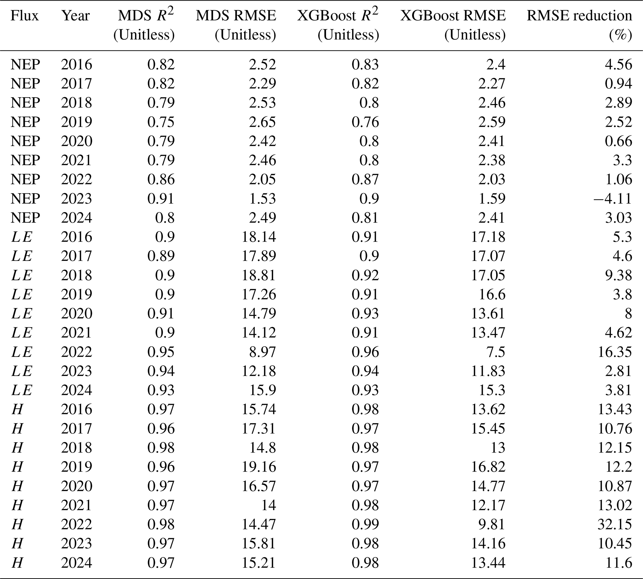
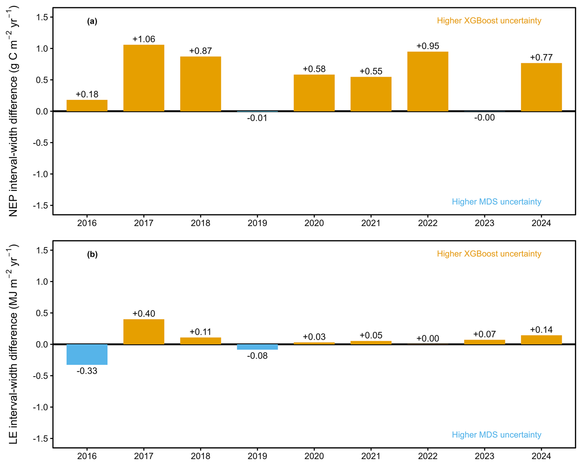
Figure C1 Interannual comparison of gap-filling prediction uncertainty between extreme gradient boosting (XGBoost) and marginal distribution sampling (MDS) from 2016 to 2024: (a) net ecosystem productivity (NEP) and (b) latent heat flux (LE). Bars show differences in the width of the 95 % Monte Carlo uncertainty interval, calculated as XGBoost minus MDS; positive and negative values indicate wider uncertainty for XGBoost and MDS, respectively.

Appendix D

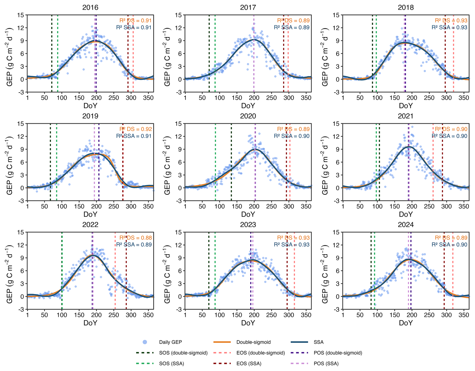
Figure D1 Comparison of double-sigmoid and singular spectrum analysis (SSA) fits used to determine the growing season from daily gross ecosystem production (GEP) during 2016–2024. Blue points show daily GEP observations. Orange lines represent the double-sigmoid seasonal curves, while dark blue lines represent the SSA-smoothed curves. Dashed lines indicate the SOS (green), EOS (red), and POS (purple) for each method. The coefficient of determination (R²) is provided for both the double-sigmoid (DS) and SSA fits in each panel.

Appendix E

Table E1 Sensitivity of growing-season boundaries and resource use efficiencies to the method used for growing-season determination during 2016–2024. Values are reported as double-sigmoid estimate / singular spectrum analysis (SSA) threshold estimate, with differences shown in parentheses. For the SSA-threshold method, daily GEP was smoothed using SSA, and SOS and EOS were defined from persistent crossings of 20 % of the annual maximum of smoothed GEP. Differences are expressed in days for SOS, EOS, and LOS, and as percentages for WUE, CUE, and LUE. Seasonal RUEs were recalculated from the original gap-filled daily fluxes within the growing-season boundaries identified by each method.

Appendix F

To evaluate the potential effect of the 9-year reference period used to calculate the Soontaga SPEI-3, an independent sensitivity analysis was conducted using meteorological data from the Tartu–Tõravere station for 2004–2024. Hourly precipitation, air temperature, global radiation, relative humidity, and wind speed were aggregated to monthly values. Potential evapotranspiration was calculated using the same Penman approach as for the site data, and the climatic water balance was standardized as SPEI at a three-month accumulation timescale. For the overlapping growing-season months of 2016–2024, the resulting Tartu–Tõravere SPEI-3 was compared with the original Soontaga SPEI-3 using Pearson and Spearman correlations, RMSE, and agreement in the sign of wet and dry conditions. To isolate the effect of reference-period length from differences between locations, SPEI-3 was also calculated from the same Tartu–Tõravere water-balance series using either the 2016–2024 or 2004–2024 reference period.

Soontaga and Tartu–Tõravere SPEI-3 were strongly correlated during the overlapping growing-season months (Pearson (r=0.83), Spearman (rho=0.82), RMSE (=0.55), (n=63)) and indicated the same wet or dry conditions in 89 % of the months. More importantly, SPEI-3 values calculated from the same Tartu–Tõravere series using the 9- and 21-year reference periods were nearly identical (r=0.98). These results indicate that the shorter reference period had little influence on the relative ranking and overall wet–dry patterns of the monthly SPEI-3 values used in the RUE analyses, although the classification of individual months near category boundaries may remain sensitive to the reference period.

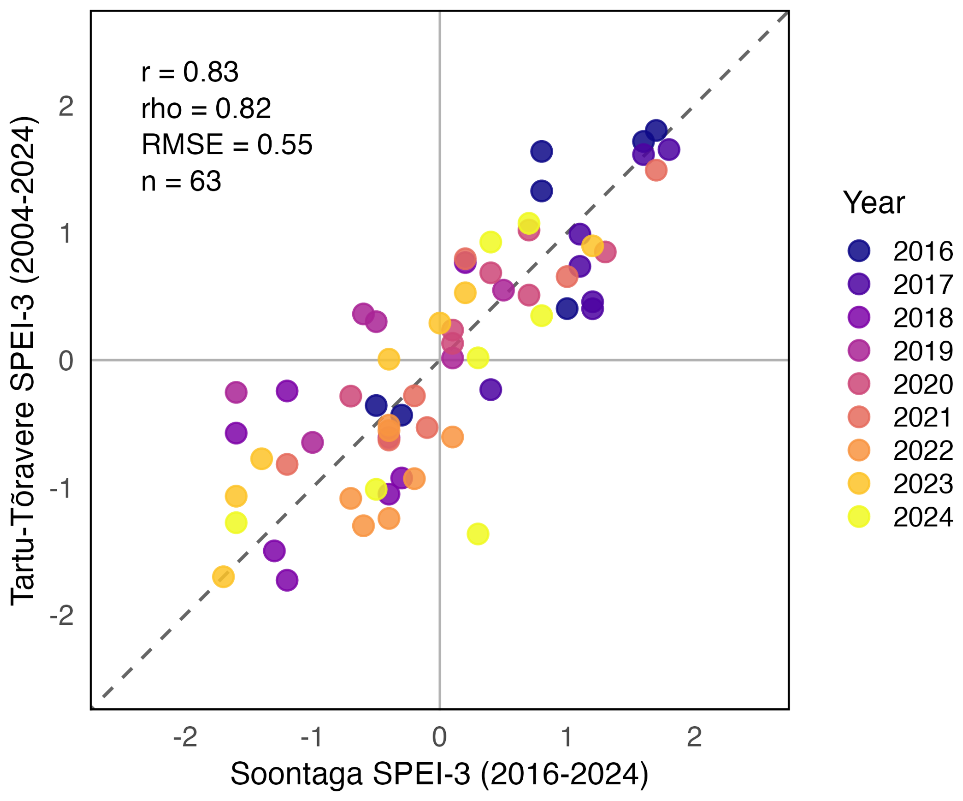
Figure F1 Comparison of Soontaga SPEI-3 calculated using the 2016–2024 reference period and Tartu–Tõravere SPEI-3 calculated using the longer 2004–2024 reference period. Points represent corresponding growing-season months (April–October) during 2016–2024, colours indicate years, and the dashed line represents the 1:1 relationship. Statistics show the Pearson correlation coefficient (r), Spearman rank correlation coefficient (rho), root mean square error (RMSE), and number of paired months (n).

To complement this robustness assessment, the median daily RUEs and their underlying carbon, water, and radiation components across the SPEI classes are presented in Table F1.

Table F1 Median daily ecosystem efficiencies and associated carbon, water, and radiation fluxes across SPEI classes. Values in parentheses indicate percentage changes relative to normal conditions.

Appendix G

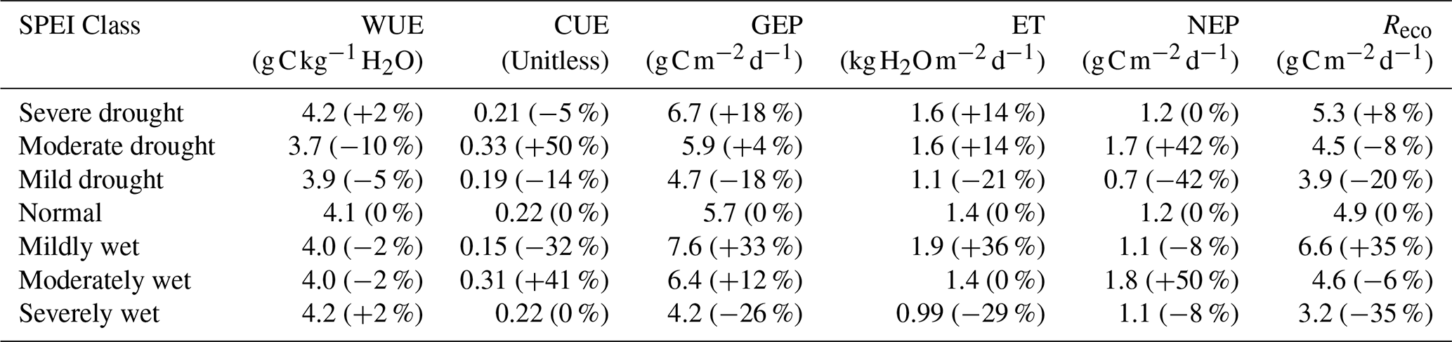
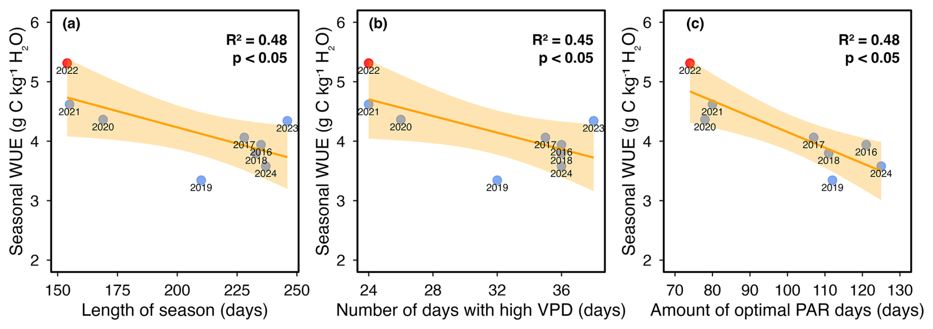
Figure G1 Relationships between growing-season water use efficiency and seasonal constraints from 2016 to 2024: (a) length of season, (b) number of high-vapour-pressure-deficit days, and (c) number of optimal-radiation days. High-vapour-pressure-deficit days are defined as days with daily VPD above the year-specific 85th percentile, and optimal-radiation days as days with daily photosynthetically active radiation (PAR) between the 25th and 75th percentiles across all years. Points show year-specific values, with 2022 highlighted. Reported R² and p values indicate the fit and significance of each linear relationship.

Appendix H

Energy balance closure was evaluated to assess the consistency of the measured fluxes and the surface energy balance. Evaluating closure is necessary because it provides a measure of how well the observed turbulent fluxes account for the available energy, thereby indicating the overall quality and reliability of the EC measurements. The lack of closure was expressed as the energy balance ratio (EBR) and slope of a linear regression model between the sum of the turbulent fluxes and the available energy (Mauder et al., 2024). EBR was calculated as the ratio between the sum of turbulent fluxes of H and LE and the available energy, defined as net radiation (R_net) minus ground heat flux (G) (Eq. H1):

$$\begin{array}{}\text{(H1)}& \text{EBR}={\displaystyle \frac{\sum H+LE}{\sum R_{\text{net}}-G}},\end{array}$$

where H is the sensible heat flux (W m⁻²), LE is the latent heat flux (W m⁻²), R_net is the net radiation (W m⁻²), and G is the ground heat flux (W m⁻²).

Ground heat flux was estimated from the soil temperature gradient between 10 and 20 cm depth using a thermal conductivity representative of sandy soils λ=0.6 $\mathrm{W}{\mathrm{m}}^{-\mathrm{1}}{\mathrm{K}}^{-\mathrm{1}}$ (O'Donnell et al., 2009). EBR was calculated separately for each year (2016–2024) using daily flux data. The EBR covered the period from 1 April to 31 October each year. Days with precipitation (precipitation >0 mm), as well as day following a precipitation event, were excluded from the analysis. We further removed days with relative humidity exceeding 80 %, air temperature below 0 °C, or low net radiation (daily integrated R_net<3.6 $\mathrm{MJ}{\mathrm{m}}^{-\mathrm{2}}{\mathrm{d}}^{-\mathrm{1}}$; ≈42 W m⁻² daily mean), as well as days with missing values in any required variables. Annual energy balance closure metrics are presented in Table H1.

Table H1 Seasonal energy balance closure metrics for each study year (2016–2024). The table reports the number of days included in the seasonal assessment, EBR, and the slope of the ordinary least squares regression between turbulent fluxes and available energy.

Appendix I

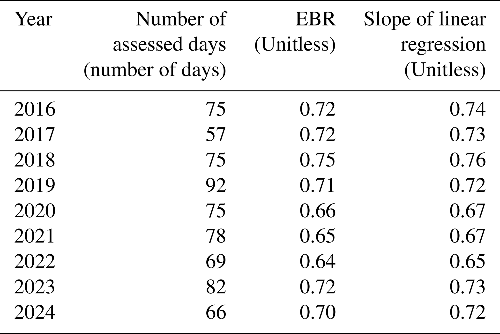
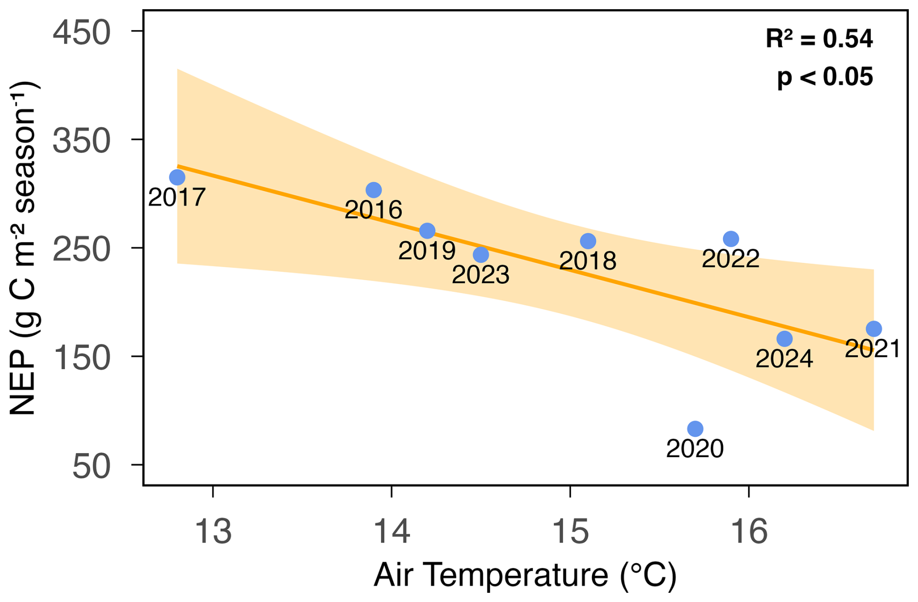
Figure I1 Interannual relationship between growing-season net ecosystem production and air temperature (2016–2024). Net ecosystem production (NEP, g C m⁻² per season) is plotted against median growing-season air temperature (T_air, °C); points show year-specific values. The orange line shows the fitted linear regression (p<0.05), and orange shading denotes the standard error of the regression.

Appendix J

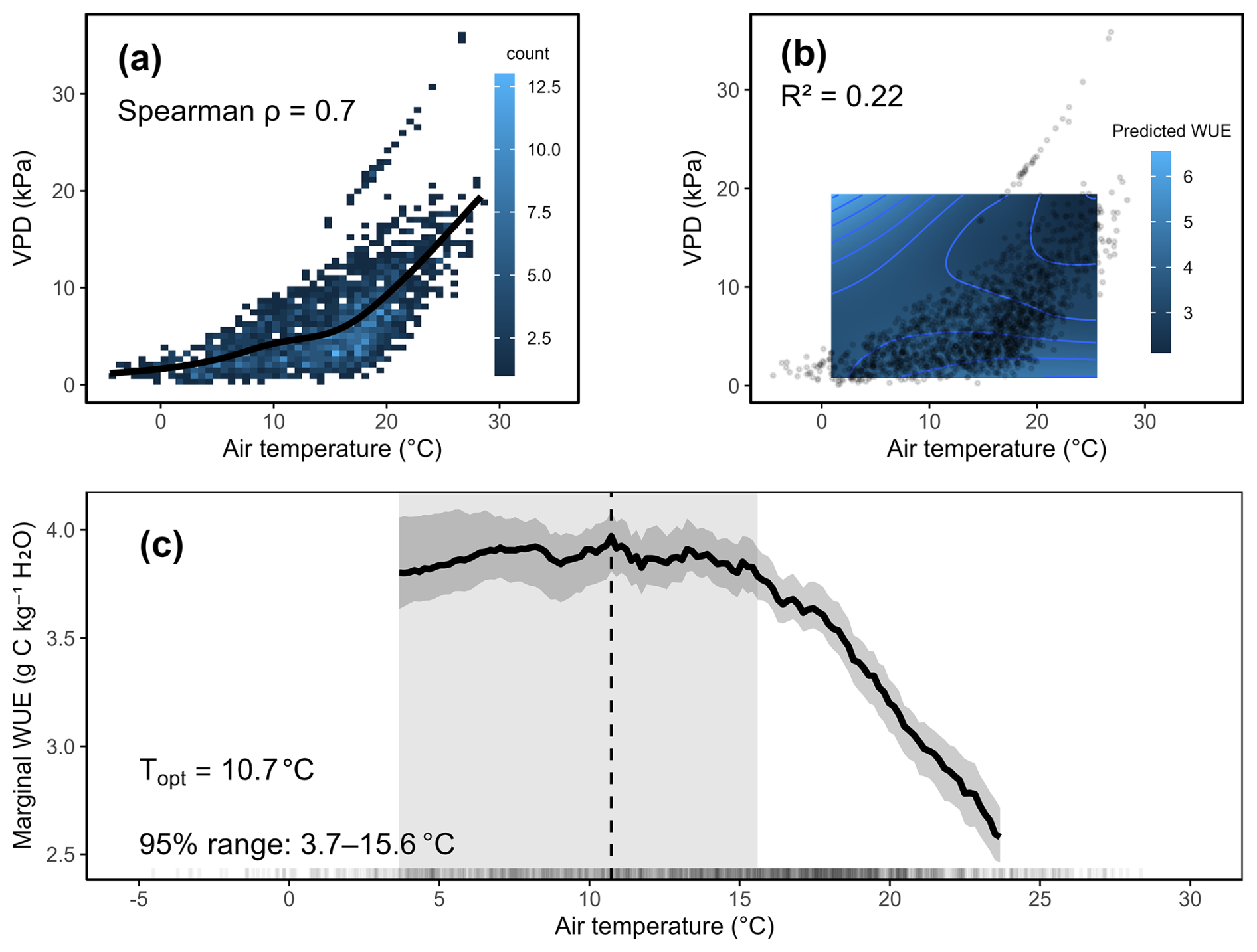
Figure J1 Air temperature–vapour pressure deficit (VPD) covariation and VPD-aware estimation of the daily water use efficiency (WUE) thermal optimum. (a) Binned relationship between air temperature and VPD, with a generalized additive model (GAM) smooth and Spearman rank correlation. (b) Joint response of daily WUE to air temperature and VPD estimated using a two-dimensional GAM; contours indicate WUE isopleths, and grey points show observed air temperature–VPD combinations. (c) VPD-aware marginal temperature response of WUE obtained by marginalising two-dimensional GAM predictions over the empirical VPD distribution within local temperature windows. The dashed line indicates the estimated optimum temperature (T_opt), the shaded band shows the near-optimal range (95 % range), and the rug indicates the distribution of observed daily temperatures.