Wheat biomass estimation across crop development using UAV LiDAR structure–intensity fusion alongside multispectral and thermal data

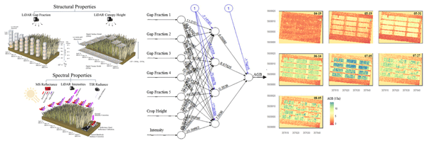
This study systematically evaluated the contribution of UAV LiDAR structural features such as crop height (CH) and multi-layer gap fraction (GF) and the amplitude of the returning signal represented by normalized intensity (INT), together with multispectral (MS) and thermal infrared (TIR) observations for aboveground biomass (AGB) estimation in winter wheat using a common artificial neural network (ANN) framework. Among the evaluated single sensor approaches, LiDAR features consistently provided the strongest performance, demonstrating the complementary value of crop height, vertically distributed canopy density, and normalized LiDAR intensity for characterizing canopy structure and within-canopy variability. Multi-layer GF improved AGB estimation relative to conventional ground-based GF approaches, highlighting the importance of incorporating the vertical distribution of canopy density. Multi-sensor fusion produced only modest additional improvements, indicating limited benefits relative to the increased acquisition and processing requirements. Temporal analysis showed that structural LiDAR features were most informative during early crop development, whereas normalized intensity, spectral reflectance, and thermal observations became increasingly valuable during canopy maturation and senescence. Comparisons with destructively measured plant area index (PAI), leaf area index (LAI), green leaf area index (GLAI), and green fraction of LAI further demonstrated that normalized LiDAR intensity (903 nm) was more closely associated with green canopy components than purely structural LiDAR metrics. Overall, the results demonstrate that fully exploiting both the structural and spectral information contained within LiDAR observations can substantially improve UAV-based biomass estimation, while multispectral and thermal observations provide complementary information whose contribution varies with crop development and monitoring objectives.

1 Introduction

Accurate and spatially explicit estimation of aboveground biomass (AGB) is essential for understanding crop development, evaluating management practices, and supporting precision agriculture through improved yield prediction and site-specific decision making (Bazrafkan et al., 2023; Lu et al., 2019). Traditional destructive sampling methods provide reliable measurements but are limited in spatial coverage and are labor-intensive, making them unsuitable for capturing within-field variability (Pan et al., 2022). While satellite remote sensing offers broader spatial data, it is limited by cloud cover, revisit times, and insufficient resolution for within-field variability (Wang et al., 2021). Manned aircraft are costly for frequent monitoring, and ground-based systems, though accurate, are constrained by limited mobility, operational risks, and potential soil compaction (Wang et al., 2021; Johansen et al., 2020). In contrast, unmanned aircraft vehicles (UAV) provide flexible, high-resolution, and on-demand data acquisition, operating below cloud cover with minimal atmospheric interference, making them ideally suited for AGB assessment in precision agriculture.

UAV platforms support an expanding array of sensor technologies, with the most common including RGB, multispectral (MS), thermal infrared (TIR), and light detection and ranging (LiDAR) systems (Bazrafkan et al., 2023). Among these, MS sensors are most widely used for biomass estimation, capturing reflectance in visible (VIS) and near-infrared (NIR) spectral bands to compute vegetation indices (VIs) that are strongly correlated with photosynthetic activity and crop vigor (Biswal et al., 2024). MS data have been widely used to estimate chlorophyll content, nitrogen status, leaf area index (LAI), fractional vegetation cover, and yield potential (Caturegli et al., 2016; Yang et al., 2018). TIR sensors, by contrast, measure land surface temperature (LST), which is closely linked to plant water stress and stomatal conductance (Ludovisi et al., 2017; Smigaj et al., 2024). When combined with meteorological data, TIR observations support the estimation of key physiological indicators such as the crop water stress index (CWSI) and evapotranspiration (ET) (Berni et al., 2009).

As opposed to the passive optical sensors, LiDAR provides three-dimensional data on crop structure and is valuable due to its ability to penetrate vegetation canopies and collect data unaffected by shadowing (Neuville et al., 2021; Wang et al., 2017). Structural properties such as crop height (CH) have shown significant promise in many cases as a strong indicator of AGB (Pan et al., 2022; Li et al., 2024; Bendig et al., 2014; Madec et al., 2017) particularly as compared to MS data, which often experiences saturation issues (Vahidi et al., 2023). With LiDAR systems being recently miniaturized enough for UAV use, they have become a more preferred method of estimating CH, offering greater precision compared to passive sensing techniques like RGB sensors and structure-from-motion (SfM) photogrammetry (Liao et al., 2021; Wallace et al., 2016). While SfM remains the more affordable alternative, LiDAR provides additional valuable outputs, including gap fraction (GF) and signal return intensities. LiDAR's ability to penetrate canopy gaps allows for the assessment of canopy density linked to LAI (Bates et al., 2021) and AGB (Montzka et al., 2023). Furthermore, the intensity of LiDAR signals, many of which operate in the NIR range (Kim et al., 2009), is influenced by canopy structure, surface properties, and vegetation condition. Previous studies have reported relationships between LiDAR intensity and green area index (GAI) (Liu et al., 2017), LAI (Luo et al., 2018), nitrogen treatment responses (Hütt et al., 2022), and vegetation classification (Mesas-Carrascosa et al., 2012; Scaioni et al., 2018; Wu et al., 2021). LiDAR intensity may therefore provide complementary information beyond purely structural metrics such as crop height and canopy density. Recent studies have likewise demonstrated its potential as an additional predictor for AGB estimation (Montzka et al., 2023; Hütt et al., 2022; Bates et al., 2022).

Integrating multiple sensor types can overcome limitations associated with individual data sources. For example, LiDAR can mitigate signal saturation issues commonly encountered in MS data, thereby improving the robustness of biomass estimation models (Tilly et al., 2015). Similarly, although TIR sensors alone often perform poorly for AGB estimation, they have been shown to enhance MS-based models when used in combination (Li et al., 2024; Maimaitijiang et al., 2017). These benefits underscore the value of sensor fusion, particularly when paired with machine learning (ML) techniques capable of handling diverse input data.

Data fusion methods increasingly rely on machine learning (ML) techniques to integrate multi-sensor information for vegetation monitoring (Li et al., 2024; Wang et al., 2024). Artificial neural networks (ANNs) are particularly well suited for this purpose because they can capture nonlinear interactions among diverse sensor features while remaining flexible for continuous regression problems (Vahidi et al., 2023). ANNs have consequently become one of the predominant approaches for crop trait and yield prediction (Van Klompenburg et al., 2020) and have demonstrated performance comparable to or exceeding that of multiple linear regression (MLR) and support vector machines (SVMs) in UAV-based agricultural applications (Dawidowicz and Buczyński, 2025; Huang et al., 2022; Kidson et al., 2025; Abu Jabed and Murad, 2024; Lionel et al., 2025). In this study, however, the ANN is not intended to identify the optimal machine learning solution for AGB estimation. Instead, it is employed as a consistent modelling framework to systematically compare the relative information content of LiDAR structural metrics, normalized intensity, multispectral reflectance, and thermal features, both individually and in combination. By maintaining a common modelling approach across all experiments, differences in predictive performance can be more directly attributed to the sensor features themselves rather than to variations in model architecture or optimization strategy.

This study systematically evaluates the contribution of UAV-derived LiDAR structural features, including crop height (CH), multi-layer gap fraction (GF), and normalized intensity (INT), together with multispectral (MS) and thermal infrared (TIR) observations for winter wheat AGB estimation. While previous studies have investigated individual LiDAR features, relatively few have systematically assessed their complementary contribution within a common modelling framework or explored the potential of multi-layer GF to represent vertical canopy heterogeneity. Rather than proposing a universally optimal biomass model, a consistent ANN framework is employed to compare the relative information content of individual sensor features and their combinations throughout the growing season. The findings provide insight into the complementary strengths and limitations of LiDAR structural metrics, normalized intensity, multispectral reflectance, and thermal observations while exploring the trade-offs between prediction performance, sensor complexity, and operational practicality under the conditions of this study.

2 Experiment Site and Setup

The experiment consisted of 12 main plots at Campus Klein Altendorf (CKA), Germany, each subdivided into six 1.5×3 m subplots. Three nitrogen fertilization treatments (0 %, 50 %, and 100 %; 50 kg N ha⁻¹ applied as a 30 % ammonium nitrate–urea solution) and three genotype classes (Trebelier, Milaneco, and a mixture of both) were arranged across the field to intentionally introduce variability in crop development, canopy architecture, and physiological status. This design generated a broad range of biomass, canopy density, and pigment conditions, providing a suitable dataset for systematically evaluating the relative contribution of different UAV-derived sensor features and their combinations. Figure 1 presents the experimental layout and sampling overview, including the spatial distribution of training and testing samples across treatment combinations. Regional flooding in July reduced the number of destructive samples available during the late-season measurement campaigns.

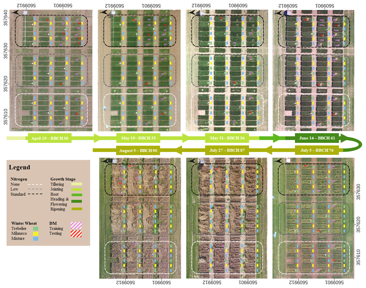
Figure 1 Study area and experimental layout at the PhenoRob Central Experiment (CKA), Germany, illustrating UAV acquisitions and destructive biomass sampling throughout the 2021 winter wheat growing season (BBCH 30–90). Orthomosaics are shown for each UAV campaign date together with the corresponding phenological growth stage. The experiment consisted of three nitrogen fertilization treatments (0 %, 50 %, and 100 %) and three winter wheat genotype categories (Trebelier, Milaneco, and a mixture of both). Destructive biomass (DM) sampling locations are indicated and color-coded according to their use for ANN model training and testing. Dashed outlines denote nitrogen treatment zones, and the arrow indicates the UAV flight direction.

AGB destructive samples were collected concurrently with UAV acquisitions between 19 April and 5 August 2021. Samples consisted of 75 cm from two interior crop rows to minimize edge effects, were dried at 60 °C for at least 48 h, and converted to t ha⁻¹. Prior to drying, samples were separated into stems, ears, and leaves, with leaf material further divided into green and senescent components. Leaf area was subsequently measured using a LI-COR LI-3000 leaf area meter, enabling determination of plant area index (PAI), leaf area index (LAI), green leaf area index (GLAI), and brown leaf area index (BLAI). Regional flooding in July reduced samples for late-season flights.

Figure 2 illustrates the destructive measurement workflow together with the temporal evolution of canopy development. The divergence between PAI and GLAI after the third sampling campaign reflects the onset of senescence, where structural biomass remains relatively constant while green leaf area rapidly declines. This provides a unique opportunity to evaluate whether different UAV-derived features respond primarily to canopy structure or to changes in green foliage.

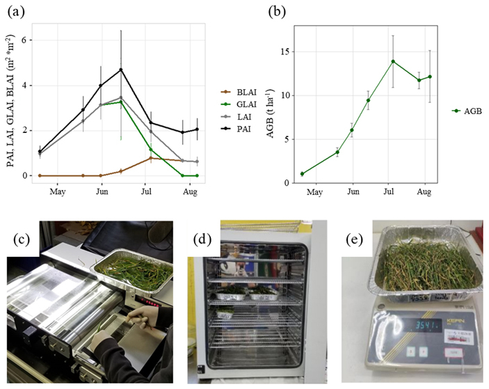
Figure 2 Destructive biomass and leaf area measurement workflow together with the temporal evolution of plant area index (PAI), leaf area index (LAI), green leaf area index (GLAI), brown leaf area index (BLAI), and above-ground biomass (AGB) (mean ± SD) throughout the 2021 winter wheat growing season. Leaf area measurements were obtained using a LI-COR LI-3000 leaf area meter following separation of green and senescent leaf components.

3 UAV Data and Pre-processing

Two DJI Matrice 600 hexacopters were used to implement a coordinated multi-sensor data acquisition workflow (Fig. 3). One platform was equipped with a YellowScan Surveyor LiDAR system, consisting of a Velodyne VLP-16 laser scanner integrated with an Applanix APX-15 GNSS/inertial navigation unit, while the second platform carried a MicaSense RedEdge-M multispectral (MS) camera together with a FLIR Vue Pro R thermal infrared (TIR) sensor mounted on a DJI Ronin gimbal.

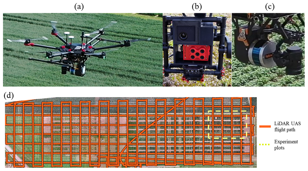
Figure 3 UAV platforms and acquisition strategy used for multi-sensor data collection. (a) DJI Matrice 600 equipped with the YellowScan Surveyor LiDAR system and DJI Zenmuse X1 RGB camera used for study site imagery; (b) FLIR Vue Pro R thermal infrared (top) and MicaSense RedEdge-M multispectral (bottom) sensors mounted on a DJI Ronin gimbal; (c) close-up of the LiDAR sensor configuration; and (d) double-grid LiDAR flight pattern used to maximize point density and viewing geometry consistency across the experimental plots.

The LiDAR system operates in the near-infrared (NIR; 896–910 nm) and records up to 300 000 pulses s⁻¹ with an approximate range precision of 4 cm. Flights were performed at 50 m above ground level and 8 m s⁻¹ using a double-grid acquisition pattern with ±25° scan angles and 50 % side overlap to maximize point density and viewing geometry consistency across the experimental plots. GNSS corrections from a Septentrio Altus NR3 base station were incorporated through Applanix POSPac and YellowScan CloudStation to generate georeferenced point clouds.

The MS sensor acquired imagery in the red (663–673 nm), red-edge (712–722 nm), and near-infrared (820–860 nm) spectral bands, while the TIR sensor recorded radiometric data between 7.5 and 13.5 µm. Both sensors were flown simultaneously at 50 m altitude and 6 m s⁻¹ using a single-grid pattern with 90 % image overlap. MS imagery was radiometrically calibrated using a reflectance panel, whereas TIR data were corrected using internal radiometric parameters (emissivity, air temperature, and relative humidity) together with a metallic blackbody reference target. An external heated shutter (TEAX ThermalCapture) was incorporated to reduce microbolometer drift and improve radiometric stability (Virtue et al., 2021). Whenever possible, UAV acquisitions were conducted near solar noon under predominantly clear-sky conditions to minimize temporal variation in illumination and atmospheric influences among campaigns. Because the experimental site was relatively small, image acquisition for each campaign could be completed rapidly under stable environmental conditions. Although some variation in meteorological conditions among acquisition dates was unavoidable, air temperature and relative humidity were recorded and incorporated into the thermal correction workflow. The thermal camera was additionally housed in an insulated 3D-printed enclosure to reduce rapid environmental fluctuations during flight, while the relatively low flight speed minimized directional effects associated with changes in aircraft orientation relative to the prevailing wind. All imagery was processed in Pix4D to generate georeferenced orthomosaics, while subsequent raster and LiDAR analyses were performed in R using the lidR and raster packages. The synchronized acquisition of LiDAR, multispectral, and thermal observations ensured that all sensor features represented comparable canopy conditions for each sampling campaign, enabling a consistent comparison of their individual and combined contributions to AGB estimation.

4 Methods

4.1 Overall Workflow

The overall methodology is summarized in Fig. 4. UAV-derived LiDAR, multispectral (MS), and thermal infrared (TIR) data were processed to generate complementary structural and spectral features for aboveground biomass (AGB) estimation. To ensure a consistent comparison among sensor types, all datasets were georeferenced, resampled, and aligned to a common spatial resolution before extracting zonal statistics corresponding to the destructive biomass sampling plots. These standardized feature sets were subsequently evaluated within a common artificial neural network (ANN) framework.

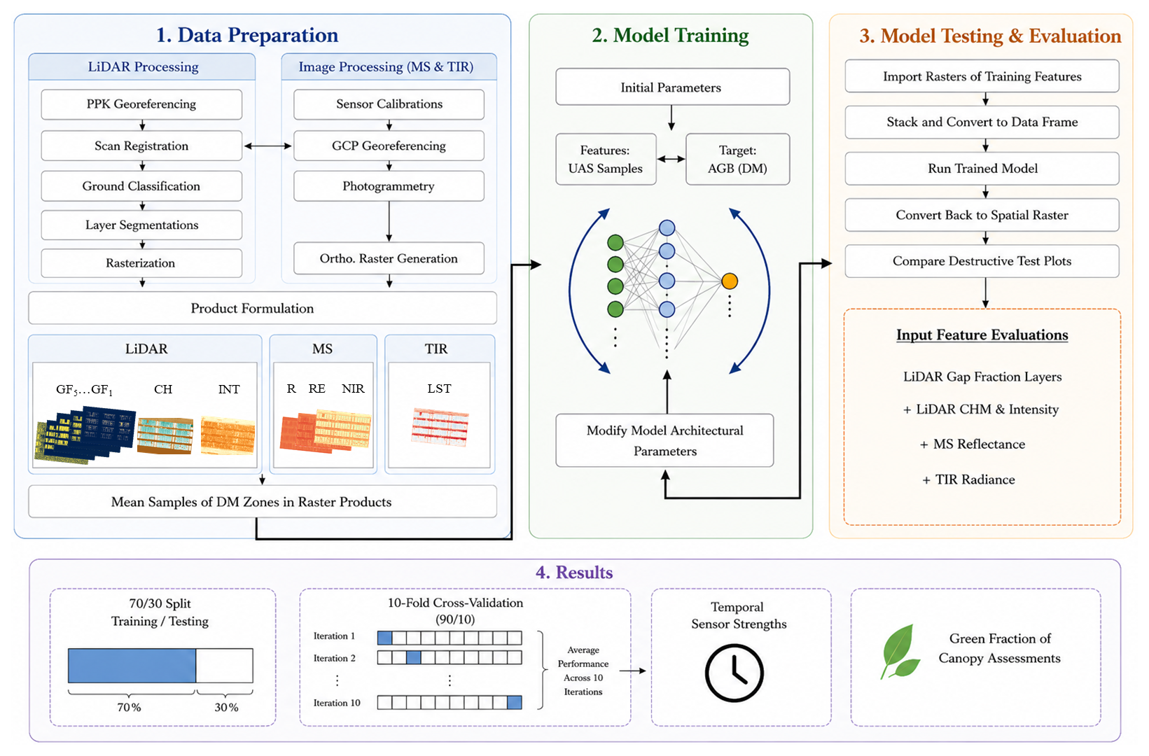
Figure 4 Overview of the methodological framework used for UAV-based aboveground biomass (AGB) estimation. UAV-derived LiDAR, multispectral (MS), and thermal infrared (TIR) observations were processed into standardized structural, spectral, and thermal feature sets and evaluated using a common artificial neural network (ANN) framework with repeated stratified cross-validation. A tiered feature addition strategy was employed, beginning with LiDAR multi-layer gap fraction (GF) and progressively incorporating crop height (CH), normalized LiDAR intensity (INT), multispectral reflectance, and thermal observations to systematically assess the complementary contribution of individual sensor features and multi-sensor combinations for winter wheat AGB estimation.

LiDAR point clouds were used to derive CH, multi-layer GF, and INT, with INT representing a wavelength-dependent return signal (903 nm) influenced by both canopy structure and vegetation surface properties, while MS and TIR imagery provided spectral reflectance and thermal radiance information (Fig. 5). Ground points were identified using the Cloth Simulation Filter (CSF) (Zhang et al., 2016) with a 4 cm grid resolution corresponding to the ranging precision of the LiDAR system. These ground returns served as the reference surface for both gap fraction calculations and intensity normalization. All raster products were converted to tabular feature sets with geographic metadata removed and normalized to a 0–1 range prior to ANN modelling. A tiered evaluation strategy was adopted to isolate the contribution of progressively more complex sensor information. The analysis began with LiDAR gap fraction using multiple vertical segmentation schemes to identify the optimal representation of canopy density (Sect. 5.1). The best-performing GF configuration was subsequently combined with crop height and normalized intensity to evaluate complementary LiDAR information (Sect. 5.2). Multispectral reflectance (Sect. 5.3) and thermal observations (Sect. 5.4) were then incrementally incorporated to quantify the additional value of multi-sensor fusion while maintaining an identical modelling framework. Following model training and validation, the selected ANN models were applied to co-registered and stacked predictor rasters using the compute() function to generate spatially continuous AGB predictions. Geographic information was subsequently reattached and the resulting biomass maps were exported as GeoTIFFs (UTM Zone 32N) for visualization and further spatial analysis.

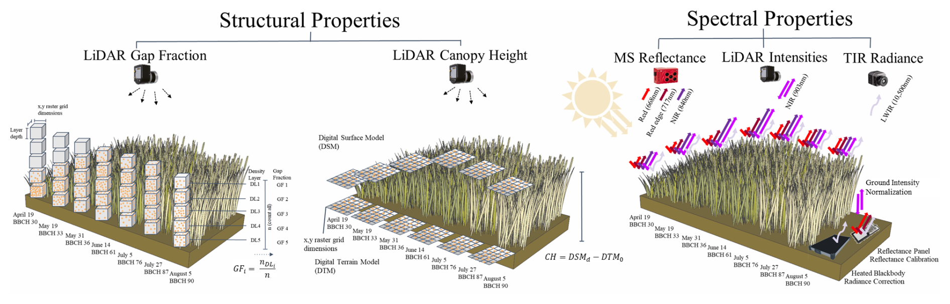
Figure 5 Conceptual representation of the UAV-derived feature groups evaluated in this study. LiDAR gap fraction and crop height represent predominantly structural canopy properties, whereas multispectral reflectance, normalized LiDAR intensity, and thermal radiance provide complementary wavelength-dependent responses influenced by both canopy structure and vegetation surface properties.

Although multispectral reflectance and normalized LiDAR intensity are both influenced by canopy structure, they were grouped as signal-based features because their recorded response depends on the interaction of electromagnetic radiation at specific wavelengths with canopy optical and surface properties. In contrast, crop height and gap fraction are derived primarily from the geometric distribution of LiDAR returns and therefore represent predominantly structural canopy attributes.

4.2 LiDAR Crop Height

CH was derived by subtracting the digital terrain model (DTM) from the digital surface model (DSM), with the DTM generated from UAV LiDAR data collected under bare-soil conditions prior to planting. This approach minimizes interpolation errors and improves accuracy (Cao et al., 2019). Several CH-derived metrics (e.g., mean, maximum, standard deviation) were tested (see Fig. B1) but the maximum CH per pixel was selected because it consistently showed stronger correlations with AGB in vertically structured, dense crops such as wheat (Bazrafkan et al., 2023). By focusing on a single robust height metric, feature redundancy and model complexity were reduced, helping to limit overfitting while maintaining a consistent comparison among sensor feature combinations (Ruwanpathirana et al., 2024). Correlations of alternative CH metrics with AGB are provided in Fig. B1.

4.3 LiDAR Multi-layer Gap Fraction

Traditional GF metrics estimate canopy density by comparing ground returns to total LiDAR returns, often within Beer–Lambert formulations for LAI estimation (Heiskanen et al., 2015; Richardson et al., 2009). However, these approaches reduce the three-dimensional canopy to a single integrated metric and can become less reliable in dense wheat canopies where laser penetration to the ground is limited (Sabol et al., 2014). To preserve vertical canopy information, we extend the GF concept by calculating normalized GF values independently for multiple canopy layers rather than relying on a single ground-based estimate. A related approach, the three-dimensional point index (3DPI), similarly partitions canopy returns into vertical layers but combines them using an empirically calibrated extinction coefficient to estimate LAI or AGB (Jimenez-Berni et al., 2018). In contrast, the normalized GF layers developed here (see Fig. 5) were incorporated directly into the ANN as independent predictor variables, allowing the model to learn the relative contribution of each canopy stratum throughout the growing season without requiring additional parameterization or extinction coefficient calibration.

Four vertical discretization schemes were evaluated, consisting of a conventional ground-only GF, three 30 cm layers, five 20 cm layers, and ten 10 cm layers. Each configuration was further assessed using horizontal grid resolutions of 10, 20, and 30 cm, selected based on the LiDAR ranging precision (∼4 cm), point density, winter wheat crop height (approximately 1–1.2 m), and subplot dimensions. For comparison, additional LiDAR canopy profile representations, including the Vertical Distribution Index (VDI), Height-Weighted Profile Index (HWPI) and 3DPI, were also evaluated in the Results. Mathematical formulations for these metrics are provided in Appendix A. The objective was not to identify a universally optimal parameterization but to systematically investigate how different representations of canopy density influence AGB estimation under the sensor characteristics, acquisition settings, and crop conditions of this study.

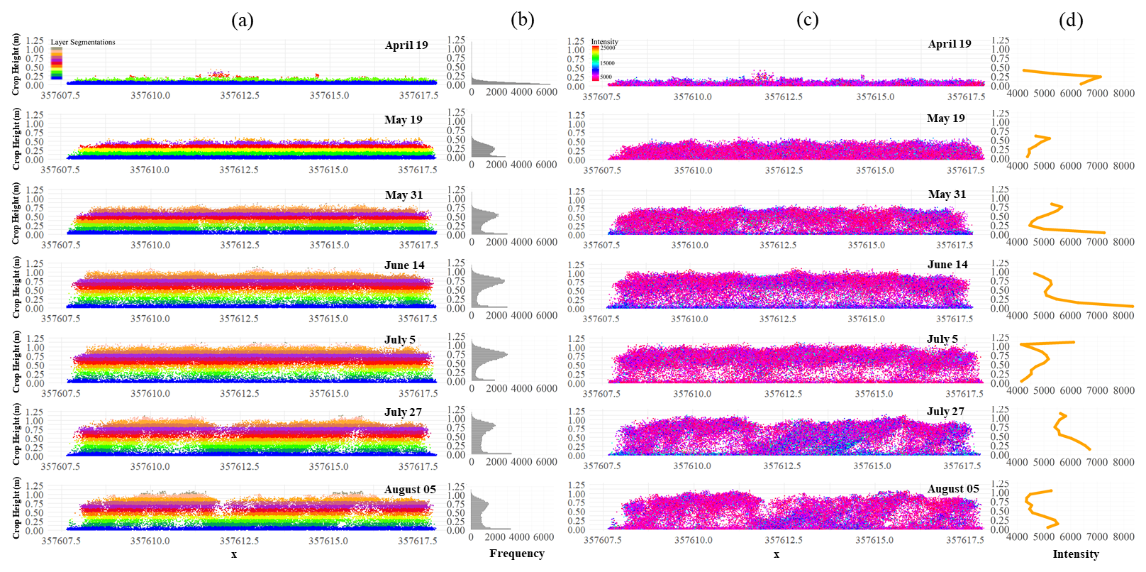
Figure 6 Seasonal evolution of LiDAR canopy structure and signal intensity for a representative winter wheat subplot. (a) Cross-sectional view of the LiDAR point cloud colored according to 10 cm vertical canopy layers used for the multi-layer gap fraction (GF) analysis. (b) Histogram showing the vertical distribution of LiDAR returns within the canopy. (c) Cross-sectional view of raw LiDAR intensity values throughout the canopy. (d) Mean LiDAR intensity profile along the vertical canopy extent. Note: Intensity values are shown prior to ground-return normalization and are included to illustrate the seasonal evolution of the LiDAR signal.

4.4 LiDAR Intensity

LiDAR intensity represents the strength of the returned laser signal at 903 nm (NIR) and, unlike crop height and gap fraction, provides a wavelength-dependent response influenced by both canopy structure and vegetation surface properties (Eitel et al., 2014). To minimize footprint variation, light dispersion, and incidence angle effects, LiDAR data were acquired using a maximum scan angle of ±25°, providing a relatively consistent viewing geometry across the experimental field (Li et al., 2016).

The temporal use of LiDAR intensity is challenging because the recorded signal is influenced not only by vegetation properties but also by environmental conditions, including soil moisture, illumination, and acquisition geometry. In the absence of dedicated reflectance targets, ground returns provide a practical reference for improving temporal consistency. Previous airborne LiDAR studies have employed ground-return normalization or related indices, such as the Light Penetration Index (LPI), to improve the estimation of vegetation structural properties including LAI (Solberg et al., 2006; You et al., 2017; Sasaki et al., 2016), while Luo et al. (2018) demonstrated the importance of accounting for ground intensity when relating LiDAR intensity to vegetation characteristics.

Several intensity representations were initially evaluated for their relationship with AGB and canopy properties (Fig. B1). Ground-return normalization produced the most consistent relationships across the spatial and temporal variability represented within the experiment and was therefore selected for subsequent analyses. The mathematical formulation of the LiDAR intensity metric used is provided in Appendix A. Although this approach does not constitute a full radiometric calibration, it provides a practical relative normalization that improves the comparability of canopy intensity measurements among acquisition dates while maintaining a simple processing workflow.

4.5 Multispectral Reflectance

MS data were collected in the red (R), red-edge (RE), and near-infrared (NIR) bands, which capture complementary information related to canopy reflectance and vegetation condition and form the basis of many commonly used vegetation indices (VIs) (Han et al., 2019). The RE band is particularly valuable because it is generally less susceptible to saturation at high biomass than the R band, providing complementary information when combined with NIR reflectance (Gitelson et al., 2003). Rather than deriving predefined VIs, the raw reflectance bands were used directly as ANN inputs. This approach avoids introducing redundancy among highly correlated indices while allowing the ANN to evaluate the relative contribution and nonlinear interactions of the individual spectral bands within a consistent modelling framework. Using the original reflectance values also preserves band-specific information that may otherwise be reduced through index formulation and facilitates a more direct comparison with LiDAR-derived structural and intensity features.

4.6 Thermal Infrared Radiance

TIR data were used to derive both land surface temperature (LST) and the crop water stress index (CWSI). LST provides an absolute measure of canopy thermal status but is strongly influenced by environmental conditions, particularly air temperature, making direct comparisons across dates and growth stages challenging. To reduce this temporal dependence, LST was additionally converted to CWSI by normalizing canopy temperature relative to seasonal “wet” and “dry” reference limits and air temperature (Katimbo et al., 2022). The mathematical formulation of the CWSI used in this study is provided in Appendix A. Both LST and CWSI were evaluated as ANN inputs to compare the contribution of absolute canopy temperature and a normalized thermal stress indicator for AGB estimation. Including both metrics enabled assessment of whether normalization improved the information content of TIR observations and provided a direct comparison between absolute and relative thermal representations within the common sensor fusion framework.

4.7 ANN Model

A multilayer perceptron ANN with backpropagation was implemented using the neuralnet package in RStudio. Model complexity (number of hidden layers and neurons) was optimized through iterative sensitivity testing, where one to two hidden layers with 2–14 neurons were evaluated. A logistic activation function was applied to the hidden neurons, while a linear activation was used for the output neuron to support continuous regression. Training employed resilient backpropagation, the default optimizer in neuralnet, which performs full-batch weight updates each iteration. Accordingly, batch size is not applicable in this framework. Training was capped using stepmax = 1×10⁶ (maximum number of weight updates) and threshold = 0.01 (convergence criterion). These settings effectively provide a high maximum number of training iterations while terminating optimization once the convergence criterion is satisfied.

A total of 86 destructive AGB samples were available for model development. This sample size reflects the constraints of destructive biomass collection, which is highly labor-intensive and logistically limited when covering an entire growing season in parallel with other field experiments (Han et al., 2019). The number and quality of destructive samples collected are comparable to those reported in UAV studies (Bendig et al., 2014; Morgan et al., 2025; Smith et al., 2024). The samples spanned seven campaigns representing major phenological stages and a wide range of canopy conditions, resulting in substantial structural and spectral variability across the growing season. Given the modest sample size, the ANN architecture was intentionally kept shallow and all predictor variables were normalized to reduce the risk of overfitting.

4.8 Model Evaluation

Model performance was evaluated using two complementary validation strategies. An initial $\mathrm{70}/\mathrm{30}$ training-testing split was used as the primary independent holdout evaluation for comparing sensor features and feature combinations (Bendig et al., 2014; Han et al., 2019; Morgan et al., 2025; Smith et al., 2024). The training and testing subsets contained observations from multiple nitrogen treatments, wheat genotypes, and measurement campaigns, with testing samples distributed across the experimental field. Model performance was assessed using RMSE and R² by comparing predictions for both the training and testing subsets, where small differences between training and testing performance indicate good generalization, whereas larger discrepancies may indicate overfitting.

A stratified 10-fold cross-validation analysis was additionally performed for selected feature combinations as a supplementary assessment of sensitivity to data partitioning. Within each fold, approximately 90 % of the observations were used for training and 10 % for validation. To account for stochastic ANN initialization, 20 networks were trained using identical architecture and training settings within each fold. Because ANN performance can vary between runs due to random initial weights, repeated initializations were used to reduce this variability and improve the consistency of comparisons among sensor combinations. The network with the lowest validation RMSE was then selected from these repeated initializations. Because the validation subset was used to select the best-performing initialization, the reported cross-validation performance may be slightly optimistic and should therefore be interpreted primarily as a comparative assessment of sensor feature combinations rather than as an estimate of model generalizability.

The cross-validation folds were stratified by measurement date but were not spatially blocked. Consequently, spatially adjacent subplots could occur in both training and validation subsets, and similar spatial dependence may also have been present within the initial $\mathrm{70}/\mathrm{30}$ training-testing split. However, the dataset incorporated substantial variability through repeated measurement campaigns spanning the growing season, multiple wheat genotypes, and contrasting nitrogen fertilization treatments distributed across the experimental field. These sources of temporal, structural, and management variability reduced the likelihood that model performance was driven solely by neighboring observations, although some influence of spatial autocorrelation could not be avoided within the relatively small experimental site. In addition, retaining the best-performing ANN initialization within each fold may have produced slightly optimistic cross-validation estimates. Consequently, the cross-validation results are interpreted primarily as a comparative assessment of feature combinations rather than as fully independent estimates of model generalizability.

5 Results

5.1 Multi-layer Gap Fraction Features and Parameter Optimization

The influence of horizontal grid resolution (GSD) and vertical layer segmentation on GF performance was systematically evaluated (Fig. 7). The tested parameter ranges were selected based on winter wheat crop height (∼1 m) and the point density achievable with the UAV LiDAR system, balancing canopy representation with sufficient point counts within each voxel.

Figure 7 Comparison of ANN performance for different LiDAR gap fraction (GF) parameterizations using varying vertical layer configurations and horizontal ground sampling distances (GSD). Bars represent training (dark green) and testing (light green) RMSE and R² values, while the dashed line indicates the corresponding GF feature complexity score, calculated as the product of the number of vertical layers and normalized GSD: Complexity = (Number of Layers) × (30 $/$ GSD in cm).

Overall, the configuration consisting of five 20 cm vertical layers and a 30 cm GSD produced the best performance (training RMSE = 2.04 t ha⁻¹, R²=0.81; testing RMSE = 2.04 t ha⁻¹, R²=0.83). Ground-only GF and coarser vertical segmentations produced moderate performance but provided limited discrimination of dense canopy structure during peak growth. Conversely, increasingly fine segmentations (10×10 cm) substantially reduced performance (testing RMSE = 7.34 t ha⁻¹; R²=0.12), likely reflecting insufficient point density within individual layers and increased model complexity.

5.1.1 Influence of Scan Angle and Point Density

Although the flight parameters (50 m altitude, double-grid pattern, 50 % overlap, and ±25° scan angle) were selected to minimize scan angle (SA) and point density (PD) variability, their potential influence on GF and AGB was further evaluated (Fig. B3 in Appendix B). Both SA and PD exhibited only weak relationships with GF and AGB (R²<0.04), indicating limited sensitivity under the acquisition conditions used in this study. Furthermore, incorporating SA or PD directly as additional ANN input features did not improve prediction performance. These results suggest that the selected acquisition parameters resulted in relatively uniform sampling conditions and that the GF formulation, which normalizes canopy returns by corresponding ground returns, largely mitigates the remaining variation associated with scan angle and point density.

5.1.2 Comparison with Existing Gap Fraction Approaches

To evaluate whether directly using multiple GF layers as ANN inputs improved biomass estimation, the proposed approach was compared with commonly used canopy density metrics including single-layer GF, 3DPI, VDI, HWPI, and multiple linear regression using the same five GF layers (Fig. 8).

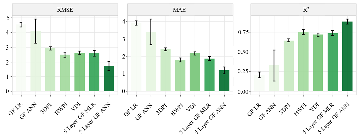
Figure 8 Comparison of cross-validation (10-fold) performance for LiDAR canopy density methods using the optimal GF parameterization identified in Fig. 7 (five 20 cm vertical layers and 30 cm GSD). Conventional single layer ground gap fraction (GF LR) was used as the baseline and compared with ANN using single GF (GF ANN), engineered multi-layer density indices (3DPI, HWPI, and VDI), multiple linear regression using the 5 layer GF (DL MLR), and the proposed 5 layer GF ANN approach. Bars represent mean performance across folds and error bars indicate variability among folds.

Using only a conventional single-layer GF provided the weakest performance (RMSE ≈4.5 t ha⁻¹; R²≈0.22). Incorporating vertical canopy information through 3DPI substantially improved prediction accuracy (RMSE ≈2.9 t ha⁻¹; R²≈0.64), with HWPI and VDI providing further modest improvements (RMSE = 2.48–2.60 t ha⁻¹; R²=0.72–0.75). These results indicate that most predictive gains arise simply from representing the vertical distribution of canopy density rather than considering only ground-visible gaps. Directly incorporating the five GF layers into a multiple linear regression model produced little additional improvement compared with engineered canopy density indices. In contrast, the ANN achieved the best overall performance (mean RMSE = 1.71 t ha⁻¹; mean R²=0.88), suggesting that nonlinear interactions among the individual canopy layers contain additional information not captured by linear combinations.

5.2 Incorporation of LiDAR Height and Intensity with Gap Fraction

Following the identification of the optimal 5 layer GF parameterization, additional LiDAR-derived features were incorporated to evaluate whether complementary structural and intensity information could further improve AGB estimation. Crop height (CH) and normalized LiDAR intensity (INT) were assessed individually and in combination with the 5 layer GF model using both the $\mathrm{70}/\mathrm{30}$ holdout evaluation and the repeated stratified 10-fold cross-validation framework (Fig. 9). Detailed $\mathrm{70}/\mathrm{30}$ training and testing scatter plots are provided in Fig. B7.

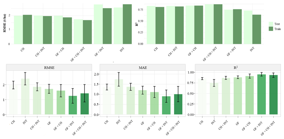
Figure 9 Performance of LiDAR-derived feature combinations for AGB estimation using the optimal 5 layer gap fraction (GF) parameterization (20 cm layer depth; 30 cm GSD). Crop height (CH), normalized intensity (INT), and 5 layer GF were evaluated individually and in combination. Top: Results from the $\mathrm{70}/\mathrm{30}$ training–testing holdout evaluation showing training (dark green) and testing (light green) RMSE and R² values. Bottom: Results from repeated stratified 10-fold cross-validation, showing mean RMSE, MAE, and R² with error bars representing variability among folds. GF refers to the 5 layer GF representation throughout this figure.

Within the $\mathrm{70}/\mathrm{30}$ holdout evaluation, CH alone provided strong predictive performance (RMSE = 1.99 t ha⁻¹; R²=0.83), substantially outperforming INT alone (RMSE = 2.56 t ha⁻¹; R²=0.73). Combining CH and INT resulted in only a marginal improvement, suggesting that crop height already captures much of the structural variability related to biomass. In contrast, incorporating either CH or INT with the 5 layer GF representation consistently improved prediction accuracy. The combination of GF + CH achieved RMSE = 1.99 t ha⁻¹ (R²=0.84), while adding INT further reduced the error to RMSE = 1.73 t ha⁻¹ with R²=0.87, representing the best-performing LiDAR-only model under the holdout evaluation.

The repeated stratified 10-fold cross-validation produced a slightly different ranking of feature combinations. Under this evaluation framework, the combination of 5 layer GF and normalized INT achieved the best overall performance (mean RMSE = 1.23 t ha⁻¹; mean R²=0.95), followed closely by the integration of CH, GF, and INT (mean RMSE = 1.41 t ha⁻¹; mean R²=0.93). In contrast, GF + INT showed comparatively weaker performance under the $\mathrm{70}/\mathrm{30}$ holdout evaluation. This difference may partly reflect the larger amount of training data available within each cross-validation fold, allowing the ANN to better exploit the complementary information contained within canopy density and intensity features. However, because the cross-validation folds were stratified by measurement date rather than spatially blocked, some influence of spatial autocorrelation between training and validation subsets may also have contributed to the higher cross-validation performance. Additional analyses showed negligible relationships between scan angle, point density, and the features used in this study (Fig. B4; R²<0.04).

5.3 Incorporation of LiDAR Metrics with MS Reflectance

Multispectral (MS) reflectance was subsequently evaluated both independently and in combination with the LiDAR-derived features to assess whether spectral information provided complementary value for AGB estimation (Fig. 10). The MS model consisted of the red (R), red-edge (RE), and near-infrared (NIR) reflectance bands and was compared with combinations of crop height (CH), 5 layer gap fraction (GF), and normalized LiDAR intensity (INT).

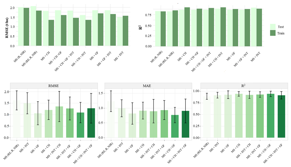
Figure 10 Biomass estimation performance using multispectral (MS) reflectance individually and in combination with LiDAR-derived crop height (CH), 5 layer gap fraction (GF), and normalized intensity (INT). The 5 layer GF configuration corresponds to the optimal parameterization identified in Fig. 7 (20 cm layer depth; 30 cm GSD). Top: $\mathrm{70}/\mathrm{30}$ holdout training and testing performance. Bottom: Repeated stratified 10-fold cross-validation showing mean RMSE, MAE, and R² with error bars representing variability among folds.

Within the $\mathrm{70}/\mathrm{30}$ holdout evaluation, MS reflectance alone produced strong predictive performance (RMSE ≈2.0 t ha⁻¹; R²≈0.83), comparable to several individual LiDAR-derived models. Integrating MS with LiDAR consistently improved biomass estimation, with the largest improvement observed for the combination of MS and normalized LiDAR intensity (RMSE ≈1.5 t ha⁻¹; R²≈0.91). Similar improvements were observed for MS combined with CH or 5 layer GF, demonstrating that passive spectral reflectance provides complementary information to LiDAR-derived canopy descriptors.

The repeated stratified 10-fold cross-validation showed a similar overall pattern while further reducing the differences among the evaluated feature combinations. The combination of MS and 5 layer GF achieved the lowest mean RMSE (1.06 t ha⁻¹) and a mean R² of 0.92, followed closely by MS + CH + 5 layer GF (RMSE = 1.09 t ha⁻¹; R²=0.94) and MS + CH (RMSE = 1.21 t ha⁻¹; R²=0.94). Although these combinations differed slightly in ranking, all LiDAR–MS models exhibited overlapping performance variability and substantially outperformed MS alone (RMSE = 1.62 t ha⁻¹; R²=0.89). The relatively small differences among the combined models suggest that the primary improvement arises from integrating complementary structural and spectral information, whereas the addition of further LiDAR-derived features provides comparatively modest gains.

Overall, these findings indicate that multispectral reflectance provides complementary information for AGB estimation, with the largest improvement achieved through its initial integration with LiDAR-derived structural features. Once complementary structural and spectral information is incorporated, additional LiDAR features provide only relatively modest improvements, suggesting diminishing returns as feature dimensionality increases under the conditions of this study.

5.4 Incorporation of LiDAR Metrics and MS Reflectance with TIR Radiance

Thermal infrared (TIR) information was subsequently evaluated independently and in combination with the LiDAR and multispectral (MS) features to assess whether canopy thermal status provided additional information for AGB estimation (Fig. 11). Both land surface temperature (LST) and the normalized crop water stress index (CWSI) were investigated individually and as complementary inputs within the sensor fusion framework.

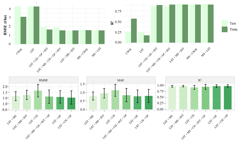
Figure 11 Biomass estimation performance using thermal infrared (TIR) features individually and in combination with multispectral (MS) and LiDAR-derived metrics. Initial comparisons include land surface temperature (LST) and crop water stress index (CWSI) as standalone predictors, after which LST was used for subsequent sensor fusion analyses. LiDAR features include crop height (CH), 5 layer gap fraction (GF), and normalized intensity (INT) using the optimal GF parameterization (20 cm layer depth; 30 cm GSD). Top: $\mathrm{70}/\mathrm{30}$ holdout training and testing performance. Bottom: Repeated stratified 10-fold cross-validation showing mean RMSE, MAE, and R² with error bars representing variability among folds.

Using TIR alone produced the weakest biomass predictions of all evaluated sensor types, with LST (RMSE = 4.27 t ha⁻¹; R²=0.25) and CWSI (RMSE = 4.26 t ha⁻¹; R²=0.26) exhibiting nearly identical performance. Because normalization to CWSI provided little additional predictive value, subsequent sensor fusion analyses focused on LST, which offers a simpler and more operationally practical metric by avoiding the need for air temperature measurements and wet/dry reference (“anchor”) pixels.

Integrating LST with LiDAR-derived features substantially improved biomass estimation. The combination of LST with 5 layer GF and normalized intensity reduced the testing RMSE to approximately 1.5 t ha⁻¹ while increasing R² to approximately 0.90, demonstrating that thermal observations provide complementary information when combined with structural canopy descriptors. Additional incorporation of multispectral reflectance or further LiDAR features produced only modest improvements, suggesting diminishing returns as feature dimensionality increased.

The repeated stratified 10-fold cross-validation showed a similar pattern, with all TIR-containing fusion models achieving consistently high predictive performance and relatively small differences among feature combinations. The combination of LST + CH + 5 layer GF produced the lowest mean RMSE (1.03 t ha⁻¹) and highest mean R² (0.95), followed closely by LST + 5 layer GF (RMSE = 1.09 t ha⁻¹; R²=0.95) and the comparatively simple LST + MS model (RMSE = 1.15 t ha⁻¹; R²=0.95). The full multi-sensor combination (LST + MS + CH + INT + 5 layer GF) achieved a mean RMSE of 1.11 t ha⁻¹ and R² of 0.92, indicating that once complementary thermal, structural, and spectral information is incorporated, additional sensor features provide only modest improvements.

Overall, these results suggest that TIR radiance serves as a complementary rather than primary predictor of AGB. While LST alone exhibits limited predictive capability, its integration with LiDAR-derived structural features and multispectral reflectance improves biomass estimation, and the minimal difference between LST and CWSI indicates that directly incorporating LST may provide a simpler and equally effective alternative for ANN-based sensor fusion under the conditions of this study.

5.5 Overall Model Comparison and Ranking of Sensor Combinations

To provide an overall comparison of the evaluated feature combinations, the top-performing single-sensor and multi-sensor models from Sect. 5.1–5.4 were ranked according to RMSE and R² for both the $\mathrm{70}/\mathrm{30}$ holdout evaluation and the repeated stratified 10-fold cross-validation (Fig. 12).

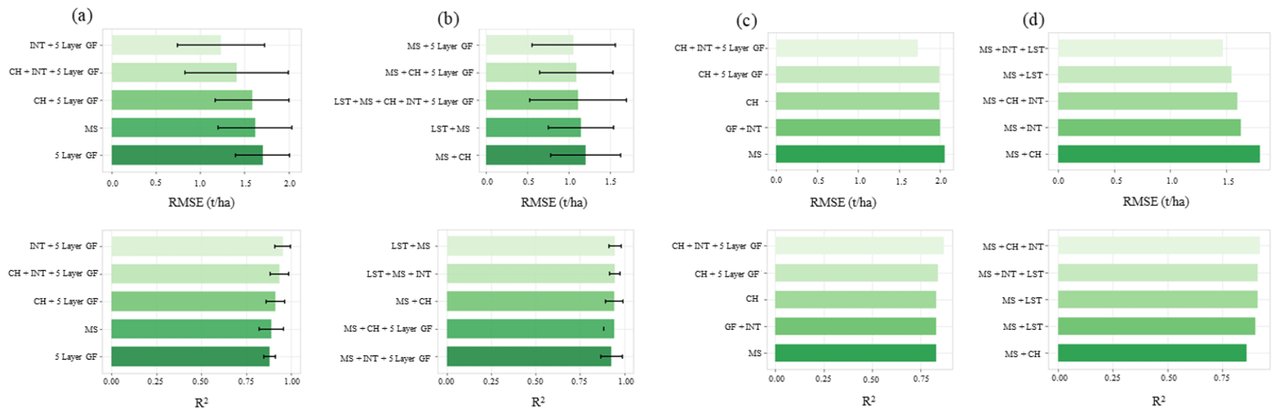
Figure 12 Ranking of the five best-performing single-sensor and multi-sensor feature combinations based on the $\mathrm{70}/\mathrm{30}$ holdout evaluation (left) and repeated stratified 10-fold cross-validation (right). Rankings are shown separately for RMSE and R². Error bars represent variability among cross-validation folds where applicable. LiDAR-derived features consistently dominate the single-sensor rankings, while several complementary LiDAR–multispectral–thermal combinations achieve similarly high performance in the multi-sensor comparison.

Across both evaluation strategies, LiDAR-derived features consistently dominated the single-sensor rankings. Models combining CH, 5 layer GF, and INT achieved the highest predictive performance, while MS reflectance also ranked among the strongest individual sensor approaches. In contrast, TIR features alone consistently produced the weakest biomass predictions, indicating that canopy temperature provides limited direct information on AGB when used independently.

The multi-sensor rankings further demonstrate the complementary nature of structural, spectral, and thermal information. Although the exact ordering of the top-performing models differed slightly between the $\mathrm{70}/\mathrm{30}$ holdout and cross-validation evaluations, all leading feature combinations incorporated information from multiple sensor types and exhibited relatively similar performance. The $\mathrm{70}/\mathrm{30}$ holdout evaluation favored combinations including MS, normalized LiDAR intensity, and LST, whereas the repeated cross-validation highlighted several LiDAR–MS feature combinations with comparable performance. Overall, LiDAR-derived information formed the foundation of every top-ranked model, with multispectral reflectance consistently providing complementary improvements and thermal observations contributing more modest gains.

5.6 AGB Estimation Evaluation by Growth Phase

To further investigate temporal sensor behavior, the best-performing single-sensor and multi-sensor feature combinations were evaluated separately for the early (19 April–31 May), mid (14 June–5 July), and late (27 July–5 August) portions of the growing season (Fig. 13). These periods correspond to distinct phases of canopy development observed in Fig. 2, including rapid vegetative growth, the divergence of LAI and GLAI during reproductive development, and complete senescence where GLAI approached zero. Additional growth-stage comparisons for all evaluated feature combinations and absolute error distributions are provided in Fig. B10.

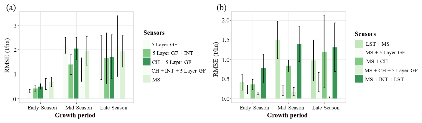
Figure 13 Growth-stage evaluation of the best-performing sensor configurations using repeated stratified 10-fold cross-validation. Left: Top five single-sensor feature combinations. Right: Top five multi-sensor feature combinations. Early season corresponds to 19 April–31 May, mid season to 14 June–5 July, and late season to 27 July–5 August. Error bars represent variability among cross-validation folds and illustrate the increasing uncertainty associated with later developmental stages.

Among the single-sensor models, LiDAR-derived structural features generally exhibited the lowest prediction errors during the early portion of the growing season, with multi-layer GF and its combinations achieving RMSE values below 0.5 t ha⁻¹. As crop development progressed and crop height approached a plateau while biomass continued to accumulate, prediction errors increased for all individual sensor approaches. The incorporation of normalized LiDAR intensity consistently improved the performance and stability of the multi-layer GF representation during the mid and late portions of the season.

Similar temporal trends were observed for the multi-sensor models. During the early portion of the season, combinations of LiDAR structural features and multispectral reflectance generally ranked among the best-performing configurations. During the mid and late portions of the season, feature combinations including multispectral reflectance together with crop height or multi-layer GF consistently exhibited low prediction errors, while combinations incorporating LST also became increasingly competitive. The larger error bars observed during the late season indicate greater variability among cross-validation folds, reflecting the increased variability present during the later stages of crop development.

5.7 Spatiotemporal alignment of UAV features with PAI, LAI, and green fraction of LAI

To further investigate the biophysical information represented by the UAV-derived features, their relationships with destructively measured canopy properties were evaluated across the major growth phases (Fig. 14). Rather than training additional ANN models, feature values extracted from the destructive sampling zones were directly compared with plant area index (PAI), leaf area index (LAI), and green fraction of LAI (f_g = GLAI $/$ LAI) using the coefficient of determination (R²). This analysis provides insight into whether individual features primarily respond to total canopy structure or to the green and photosynthetically active component of the canopy.

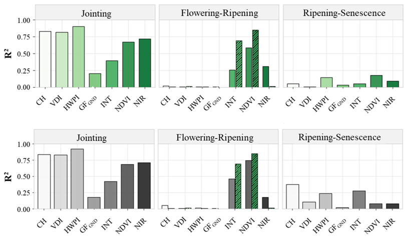
Figure 14 Relationships (R²) between UAV-derived features and destructively measured canopy properties across three major growth periods. The top row compares feature responses with leaf area index (LAI) and, during flowering–ripening, green fraction of LAI (f_g = GLAI $/$ LAI; striped bars). The bottom row compares the same features with plant area index (PAI). Only representative LiDAR canopy density metrics (GF_GND, VDI, and HWPI) together with crop height (CH), normalized LiDAR intensity (INT), NDVI, and NIR reflectance are shown for clarity. GF_GND refers to the conventional single-layer ground-based GF method.

During the jointing stage, when the canopy consisted almost entirely of green vegetation (GLAI ≈ LAI and f_g≈1), the structural LiDAR metrics exhibited the strongest relationships with both PAI and LAI (Fig. 14). Crop height (CH), VDI, and particularly HWPI showed high correspondence with the destructive measurements (R²≈0.82–0.91), whereas the conventional ground-based GF performed substantially worse. These results highlight the advantage of preserving vertical canopy information during early crop development. During the flowering–ripening stage, the relationships changed markedly as LAI diverged from GLAI while PAI remained relatively stable (Fig. 2). Purely structural LiDAR metrics exhibited little correspondence with LAI or f_g, whereas normalized LiDAR intensity showed the strongest relationship with f_g and multispectral NDVI displayed a similar response. This suggests that the 903 nm LiDAR return captures complementary information related to canopy greenness and physiological condition beyond geometric structure alone. During the ripening–senescence stage, when GLAI approached zero and f_g was no longer meaningful, structural LiDAR metrics again exhibited modest relationships with PAI, particularly HWPI, indicating that changes in canopy architecture remained detectable even as green vegetation declined. Spectral relationships were generally weaker during this period.

Overall, the correspondence between UAV-derived features and destructive canopy measurements varied with crop development. Structural LiDAR metrics were most informative during jointing and ripening, whereas normalized LiDAR intensity and multispectral NDVI exhibited the strongest relationships with green canopy fraction during flowering–ripening. These complementary temporal responses help explain the sensor fusion results, where structural features dominated biomass estimation early in the season while intensity and multispectral observations provided the greatest additional value as the canopy matured and senesced.

6 Discussion

6.1 Enhancing AGB Estimation through Improved LiDAR Feature Representation

Among the evaluated UAV features, LiDAR-derived structural metrics consistently ranked among the strongest predictors of AGB throughout the growing season. In particular, representing canopy density using multiple vertical GF layers substantially improved biomass estimation compared with the conventional ground-return GF approach commonly used for LAI estimation (Bates et al., 2021; Dreier et al., 2024) and more recently for AGB estimation (Montzka et al., 2023; Hütt et al., 2022). These findings demonstrate that preserving within-canopy structural information provides a more complete representation of crop architecture than a single integrated canopy density metric.

The parameter sensitivity analysis further showed that increasing structural detail improves biomass estimation only while sufficient LiDAR sampling density is maintained. Under the acquisition conditions of this study, the five-layer (5×20 cm) GF representation combined with a 30 cm ground sampling distance provided the best balance between canopy characterization and point density, whereas finer 10×10 cm discretization likely contained insufficient returns within individual layers for robust density estimation. Rather than representing a universally optimal configuration, the appropriate layer depth and number should be selected according to sensor performance, flight parameters, resulting point density, and crop canopy structure.

The complementary nature of the LiDAR features was further demonstrated when CH, multi-layer GF, and normalized INT were evaluated together. CH describes overall canopy development, while multi-layer GF characterizes the vertical distribution of canopy density and remained sensitive to within-canopy structural variation after crop height had largely stabilized. Temporal comparisons with destructive measurements further showed that structural LiDAR features exhibited the strongest relationships with PAI and LAI during early development, providing a physical explanation for their consistently strong biomass prediction performance.

Overall, these results highlight the importance of feature design for UAV-based biomass estimation. While most UAV LiDAR biomass studies have relied primarily on crop height as the dominant structural predictor (Bendig et al., 2014; Madec et al., 2017; Pan et al., 2022), our results demonstrate that incorporating vertically resolved canopy density and normalized LiDAR intensity provides complementary information that better captures canopy heterogeneity and seasonal dynamics. Rather than relying solely on increasingly complex machine learning architectures, improving the physical representation of canopy structure through optimized LiDAR features produced substantial gains in predictive performance while maintaining direct links to measurable crop properties.

6.2 LiDAR Intensity as a Complementary UAV Feature

Compared with crop height and canopy density metrics, UAV LiDAR intensity has received relatively limited attention for crop biomass estimation despite being acquired simultaneously with the three-dimensional point cloud. Previous studies have reported relationships between LiDAR intensity and canopy properties including LAI (Luo et al., 2018), green area index (Liu et al., 2017), nitrogen treatments (Hütt et al., 2022), and AGB (Montzka et al., 2023). Consistent with these findings, normalized LiDAR intensity in the present study consistently improved biomass estimation when combined with crop height and multi-layer gap fraction. Because intensity is inherently recorded during LiDAR acquisition and the simple ground-based normalization adopted here improved temporal consistency without requiring full radiometric calibration, it represents a practical complementary feature that can be extracted without additional sensors or acquisition costs.

The temporal analyses provide further insight into this complementary behavior. During the flowering–ripening period, when crop height had largely stabilized and PAI diverged from LAI and GLAI, normalized LiDAR intensity maintained stronger relationships with LAI and, particularly, the green fraction of LAI than the purely structural LiDAR metrics. This complementary response may reflect the influence of both canopy density (Hütt et al., 2022) and leaf orientation and surface optical properties on the 903 nm return signal (Tian et al., 2021), helping explain why intensity was retained in many of the highest-performing LiDAR-only and multi-sensor feature combinations.

6.3 Benefits of Multi-Sensor Fusion Across Phenological Stages

Multi-sensor fusion consistently improved AGB estimation compared with individual sensor approaches, supporting previous studies that demonstrate the value of combining complementary structural, spectral, and thermal information for crop monitoring (Li et al., 2024; Maimaitijiang et al., 2017; Wang et al., 2024). However, the magnitude of these improvements depended on both the selected feature combination and crop phenology.

Temporal analyses showed that LiDAR-derived structural features provided the strongest predictions during early vegetative development, whereas multispectral reflectance and normalized LiDAR intensity became increasingly valuable during the flowering–ripening period when crop height had largely stabilized and PAI diverged from LAI and GLAI. Thermal information produced comparatively modest improvements but consistently enhanced several of the highest-performing fusion models, indicating that physiological information provides complementary value when combined with structural and spectral observations.

Despite these benefits, many of the highest-performing fusion models exhibited very similar predictive performance despite differing substantially in sensor complexity. These results suggest diminishing returns as additional sensors or derived features are incorporated and emphasize the flexibility of a feature-based fusion framework. Rather than identifying a universally optimal sensor configuration, the findings indicate that sensor selection should be guided by the objectives and logistical constraints of the monitoring campaign, balancing prediction accuracy against acquisition cost, payload requirements, processing complexity, and operational practicality.

6.4 Practical Implications for UAV-Based Biomass Monitoring

The results demonstrate the practical potential of UAV LiDAR for high-resolution biomass monitoring. A single LiDAR acquisition simultaneously provides complementary information describing overall canopy development (CH), the vertical distribution of canopy density (multi-layer GF), and normalized return intensity (INT), producing some of the highest-performing biomass models while requiring only a single sensor and acquisition workflow.

Figure 15 further illustrates this advantage by comparing UAV-derived AGB, destructive biomass measurements, and grain yield across nitrogen fertilization treatments throughout the growing season. While both UAV and destructive measurements captured similar temporal dynamics and treatment responses, the UAV estimates exhibited smoother transitions and lower variability because they represent entire treatment plots rather than a limited number of sampling quadrats. This spatial completeness provides a more representative characterization of treatment effects and within-field variability while reducing the influence of localized sampling heterogeneity; spatial AGB maps across all UAV acquisition dates are provided in Fig. B11.

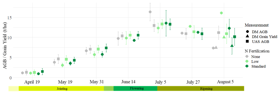
Figure 15 Comparison of UAV-derived above-ground biomass (AGB), destructive AGB measurements, and grain yield across nitrogen fertilization treatments throughout the winter wheat growing season. UAV estimates were generated using the combined crop height (CH), 5 layer gap fraction (GF), and field-normalized LiDAR intensity (INT) model and represent the entire treatment plots, whereas destructive AGB measurements were obtained from discrete subplot sampling locations. Error bars indicate ± SD within each nitrogen treatment. The figure illustrates the ability of UAV observations to capture seasonal biomass dynamics and nitrogen treatment responses while providing spatially continuous estimates beyond the limited destructive sampling locations.

From an operational perspective, the highest-performing multi-sensor models differed only marginally in prediction accuracy, suggesting that sensor selection should be guided by the broader objectives of the monitoring campaign rather than biomass estimation alone. For AGB-focused applications, LiDAR-derived structural features and normalized intensity may provide sufficient information, whereas multispectral or thermal sensors can be incorporated when additional products such as nutrient status, pigment content, evapotranspiration, or water stress are also required. Rather than replacing other sensing technologies, the results suggest that LiDAR forms a strong foundation onto which complementary sensors can be added according to the agronomic objectives and logistical constraints of individual monitoring campaigns.

6.5 Limitations and Future Directions

The primary objective of this study was to systematically compare UAV-derived feature representations within a consistent ANN framework rather than to identify a universally optimal biomass prediction model. Consequently, the findings should be interpreted within the context of the winter wheat canopy structure, management practices, sensor configuration, and environmental conditions investigated here. Future studies should evaluate these feature combinations across additional crops, sites, growing seasons, and machine learning frameworks, as sensor performance is likely to vary with canopy architecture (e.g., grasses vs. broadleaf crops) and modelling approach (Han et al., 2019; Sharma et al., 2022; Bazrafkan et al., 2023).

The validation framework also has limitations. Although the dataset incorporated substantial temporal and management variability, the relatively small experimental field meant that some influence of spatial autocorrelation between training and validation samples could not be entirely avoided. Because the primary objective of this study was to compare the relative performance of individual sensors and their fusion rather than develop a universally transferable biomass model, these results provide a valuable starting point for systematic sensor comparison. Future studies should further evaluate the proposed sensor metrics using spatially blocked cross-validation and independent sites or growing seasons to better assess model transferability and feature generalizability.

The results also highlight opportunities for further LiDAR feature refinement. While the 5 layer GF representation consistently outperformed conventional single-layer approaches, future studies should investigate adaptive layer parameterization based on canopy structure, sensor characteristics, and acquisition settings rather than fixed layer depths. Similarly, radiometrically calibrated LiDAR intensity, which was not evaluated here, may further improve temporal consistency and strengthen the physical interpretation of intensity measurements. The weak relationships observed between scan angle, point density, GF, and AGB (see Figs. B3 and B4) suggest that the low-altitude, ±25° acquisition strategy effectively minimized these influences, although they may become increasingly important under wider scan angles, lower point densities, or more complex terrain.

Finally, extending vertically segmented features beyond canopy density represents a promising research direction. Multi-layer LiDAR intensity profiles could help separate structural and radiometric effects within the canopy, improving the estimation of green canopy fraction and providing complementary information for biomass estimation and other applications such as evapotranspiration modelling. Future multispectral or multi-wavelength LiDAR systems (Takhtkeshha et al., 2024) may further capitalize on these concepts by enabling vertically resolved vegetation indices that characterize within-canopy surface conditions in addition to structure. Combined with appropriate radiometric calibration and methods to disentangle the effects of canopy density, leaf angle, and viewing geometry, such systems could provide new physically meaningful features for precision agriculture and crop monitoring.

7 Conclusion

This study systematically evaluated the contribution of UAV-derived LiDAR structural features, normalized LiDAR intensity, multispectral reflectance, and thermal infrared observations for aboveground biomass estimation in winter wheat within a common ANN framework. Particular emphasis was placed on assessing multi-layer gap fraction (GF) and normalized LiDAR intensity, two LiDAR-derived features that remain comparatively underexplored for crop biomass monitoring.

Within the conditions of this study, LiDAR-derived features generally provided the strongest single-sensor performance. Representing canopy density using multiple vertical GF layers substantially improved biomass estimation compared with conventional ground-only approaches, while normalized LiDAR intensity consistently provided complementary information to crop height and GF throughout the growing season. Temporal comparisons with destructive PAI, LAI, GLAI, and green fraction measurements further demonstrated that the correspondence between UAV features and canopy properties changed with crop development. Notably, normalized LiDAR intensity exhibited a much stronger relationship with the green fraction of LAI than the purely structural LiDAR metrics (CH and GF), which showed little to no correspondence during the flowering–ripening period. This finding highlights the potential of LiDAR return intensity, measured at a wavelength centered on 903 nm, to provide complementary information beyond canopy structure alone.

Multi-sensor fusion further improved biomass estimation, although the differences among the highest-performing feature combinations were relatively small. These results suggest that LiDAR-derived information forms a strong foundation for UAV biomass estimation, while multispectral and thermal observations provide complementary improvements whose value depends on the broader objectives of the monitoring campaign rather than biomass estimation alone. The high-resolution biomass maps also demonstrated the ability of UAV observations to provide spatially continuous information beyond that obtainable from limited destructive sampling, supporting applications such as precision nutrient management and field-scale crop monitoring.

Overall, the results emphasize that improving physically meaningful feature representations may be as important as increasing machine learning complexity. Beyond crop height alone, the combination of multi-layer canopy density and normalized LiDAR intensity highlights the untapped potential of LiDAR-derived features for agricultural monitoring and provides a foundation for future developments including radiometrically calibrated and multi-wavelength LiDAR systems capable of integrating structural and spectral canopy information within a single sensing platform.

Appendix A: Feature Definitions and Equations

Appendix A provides the mathematical definitions of the principal LiDAR-derived structural metrics, normalized LiDAR intensity, and thermal indices used throughout the manuscript. Additional model results, sensitivity analyses, scatter plots, and supplementary figures are provided in Appendix B.

A1 Multi-Layer Gap Fraction (GF)

The multi-layer gap fraction (GF) used in this study represents the relative proportion of LiDAR returns contained within each vertical canopy layer rather than a conventional optical gap fraction. By normalizing the number of returns within a layer by the total number of returns inside the corresponding grid cell, the metric describes the vertical distribution of canopy density while remaining independent of the absolute point density.

$$\begin{array}{}\text{(A1)}& {\text{GF}}_i={\displaystyle \frac{n_{{\mathrm{DL}}_i}}{n}}\end{array}$$

where $n_{{\mathrm{DL}}_i}$ is the number of LiDAR returns within density layer i and n is the total number of LiDAR returns within the corresponding grid cell. For the five-layer implementation used in this study, GF = [GF₁, GF₂, GF₃, GF₄, GF₅].

A2 Adapted Three-Dimensional Profile Index (3DPI)

The Three-Dimensional Profile Index (3DPI) proposed by Jimenez-Berni et al. (2018) was adapted in this study to use the multi-layer gap fraction (GF_i) representation described above. The resulting formulation applies an exponential weighting to the vertical canopy density profile, emphasizing returns from progressively higher canopy layers according to an optimized extinction coefficient (k):

$$\begin{array}{}\text{(A2)}& \mathrm{3}\text{DPI}=\sum _{i=\mathrm{1}}^n{\text{GF}}_i{e}^{k\cdot {\mathrm{pcs}}_i}\end{array}$$

where pcs_i is cumulative fraction of points intercepted above layer i, k is the extinction/correction coefficient, and n is the number of vertical layers. In this study, the 3DPI formulation was adapted to the five-layer, 20 cm vertical GF configuration, and k was optimized by brute-force cross-validation. The best-performing correction factor was k=1.65.

A3 Vertical Distribution Index (VDI)

The Vertical Distribution Index (VDI) is an entropy-inspired metric introduced in this study to quantify the vertical heterogeneity of LiDAR returns within the canopy. Rather than emphasizing total canopy density, the metric describes how evenly LiDAR returns are distributed among the vertical layers, with larger values indicating a more heterogeneous canopy profile and smaller values indicating that returns are concentrated within fewer layers.

$$\begin{array}{}\text{(A3)}& \text{VDI}=-\sum _{i=\mathrm{1}}^n{\text{GF}}_i\ln \left({\text{GF}}_i\right)\end{array}$$

where GF_i is the proportion of LiDAR returns contained within vertical layer i (GF_i = number of LiDAR points within vertical layer $/$ total number of LiDAR points across all layers), n is the total number of vertical layers (five 20 cm layers in this study). Unlike the adapted 3DPI, VDI contains no empirical weighting coefficient (k), making it a purely statistical description of the vertical distribution of LiDAR returns.

A4 Height-Weighted Profile Index (HWPI)

The Height-Weighted Profile Index (HWPI) is a profile-based metric introduced in this study to describe the vertical distribution of LiDAR returns while assigning greater importance to returns located higher within the canopy. Unlike VDI, which characterizes the heterogeneity of the vertical return distribution, HWPI represents the mean normalized vertical position of LiDAR returns within the canopy profile.

$$\begin{array}{}\text{(A4)}& \text{HWPI}=\sum _{i=\mathrm{1}}^n{\text{GF}}_i{h}_i\end{array}$$

where h_i is the normalized height weighting assigned to layer (i). In this study, five 20 cm layers were used with normalized height weights of 0.10, 0.30, 0.50, 0.70, and 0.90 from the lowest to highest canopy layer, respectively. Larger HWPI values indicate that a greater proportion of LiDAR returns originate from the upper canopy, whereas lower values indicate that returns are concentrated nearer the lower canopy.

A5 Normalized LiDAR Intensity (INT)

The normalized LiDAR intensity (INT) used in this study was calculated by dividing the mean vegetation intensity within each grid cell by the mean ground intensity calculated from all ground grid cells across the experimental field.

$$\begin{array}{}\text{(A5)}& {\mathrm{INT}}_{\mathrm{norm}}={\displaystyle \frac{{\stackrel{\mathrm{‾}}{\text{INT}}}_{\mathrm{grid}}}{{\stackrel{\mathrm{‾}}{\text{INT}}}_{\mathrm{ground}}}}\end{array}$$

where ${\stackrel{\mathrm{‾}}{\text{INT}}}_{\mathrm{grid}}$ is the mean LiDAR intensity of all returns contained within the corresponding grid cell, and ${\stackrel{\mathrm{‾}}{\text{INT}}}_{\mathrm{ground}}$ is the mean LiDAR intensity of all ground-classified grid cells across the study area for the same acquisition date. The resulting normalized intensity is dimensionless, with values representing the relative canopy reflectance compared with the field-average ground reference.

A6 Crop Water Stress Index (CWSI)

The Crop Water Stress Index (CWSI) was calculated by normalizing the canopy–air temperature difference (LST − T_air) between lower and upper reference limits:

$$\begin{array}{}\text{(A6)}& \text{CWSI}={\displaystyle \frac{\left(\text{LST}-T_{\mathrm{air}}\right)-\text{LL}}{\text{UL}-\text{LL}}}\end{array}$$

where LST is the land surface temperature, T_air is the air temperature at the time of UAV acquisition, LL is the lower reference limit representing fully transpiring condition, and UL is the upper reference limit representing the non-transpiring condition. In this study, LL and UL were derived from seasonal canopy temperature extremes following Katimbo et al. (2022).

A7 Crop Height (CH)

Crop height (CH) was calculated as the difference between the Digital Surface Model (DSM) acquired for each campaign and the pre-season Digital Terrain Model (DTM):

$$\begin{array}{}\text{(A7)}& \text{CH}={\text{DSM}}_d-{\text{DTM}}_{\mathrm{0}}\end{array}$$

where DSM_d is the Digital Surface Model corresponding to acquisition date d, and DTM₀ is the Digital Terrain Model representing the bare soil surface prior to vegetation growth.

Appendix B: Supplementary Results

Appendix B provides supplementary analyses supporting the principal findings presented in the main manuscript. These results are included to improve transparency and reproducibility while maintaining the readability of the primary text.

B1 Correlation Analysis of Candidate LiDAR Metrics

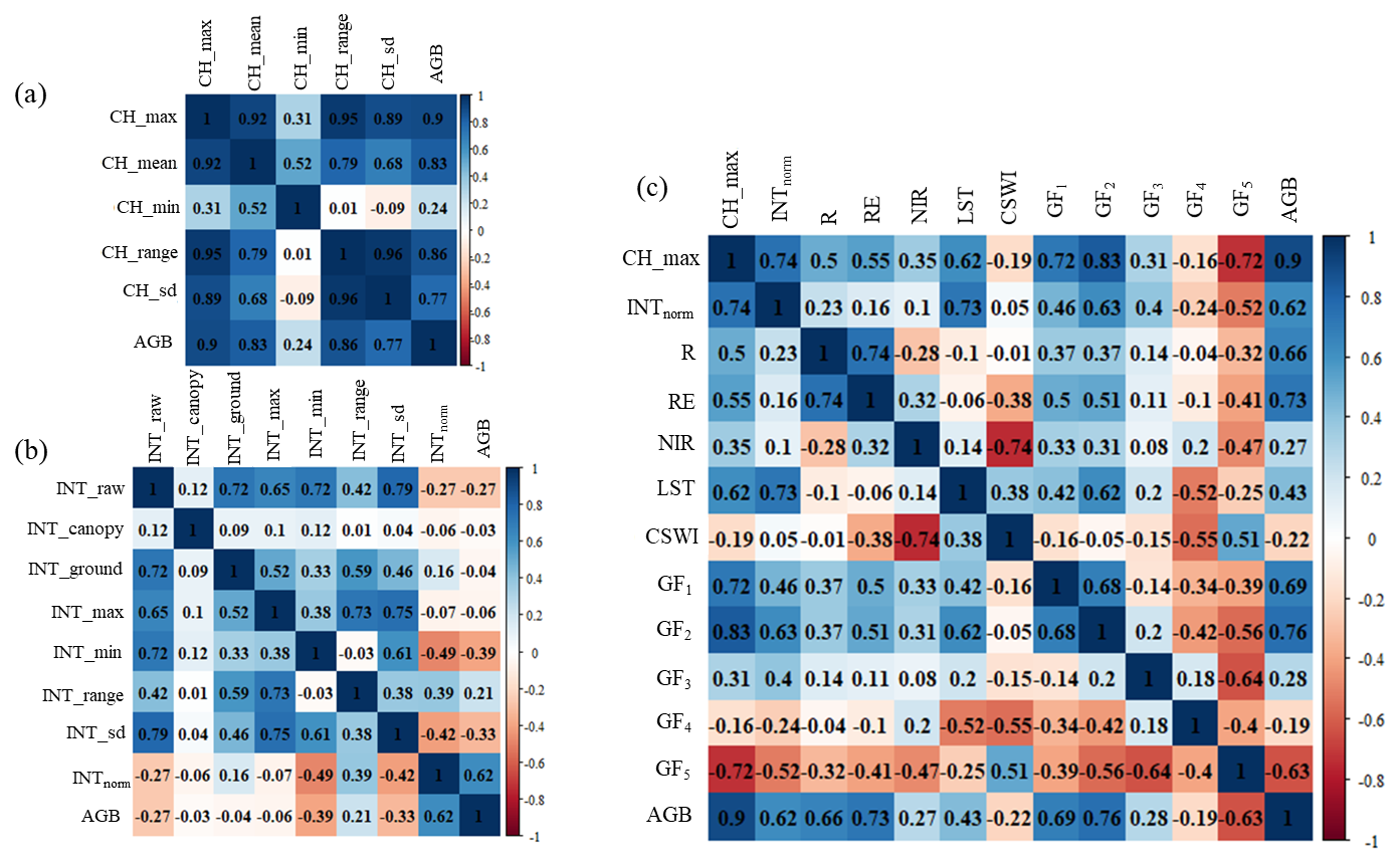
Figure B1 Correlation analysis of candidate UAV sensor features with above-ground biomass (AGB). (a) LiDAR crop height (CH) metrics, including maximum, mean, minimum, standard deviation, and range. (b) LiDAR intensity (INT) metrics, including raw intensity (INT_raw), canopy-only (INT_canopy), and ground-only intensity (INT_ground), maximum, minimum, range, standard deviation, and intensity normalized by the average ground intensity across the study area (INT_norm). (c) Correlation of the best-performing LiDAR metrics (CH_max and INT_norm) with multispectral reflectance bands (Red, Red-edge, and NIR), thermal products (LST and CWSI), and the five 20 cm LiDAR gap fraction layers (GF₁ − GF₅). These comparisons were used to support the selection of representative features for subsequent model development.

B2 Temporal Evolution of UAV-Derived Features

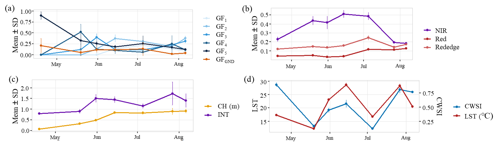
Figure B2 Temporal evolution of UAV-derived canopy features throughout the winter wheat growing season. Mean values (± SD) are shown for (a) the five 20 cm LiDAR multi-layer gap fraction layers (GF₁ − GF₅) together with the conventional ground-based gap fraction (GF_GND), (b) multispectral reflectance bands (Red, Red-edge, and NIR), (c) LiDAR maximum crop height (CH) and normalized LiDAR intensity (INT), and (d) thermal products including the Crop Water Stress Index (CWSI) and land surface temperature (LST). The temporal trajectories illustrate changes in canopy structure, spectral response, LiDAR intensity, and thermal status across the growing season, providing context for the observed phenological shifts in sensor contributions to above-ground biomass estimation.

B3 Influence of Scan Angle and Point Density

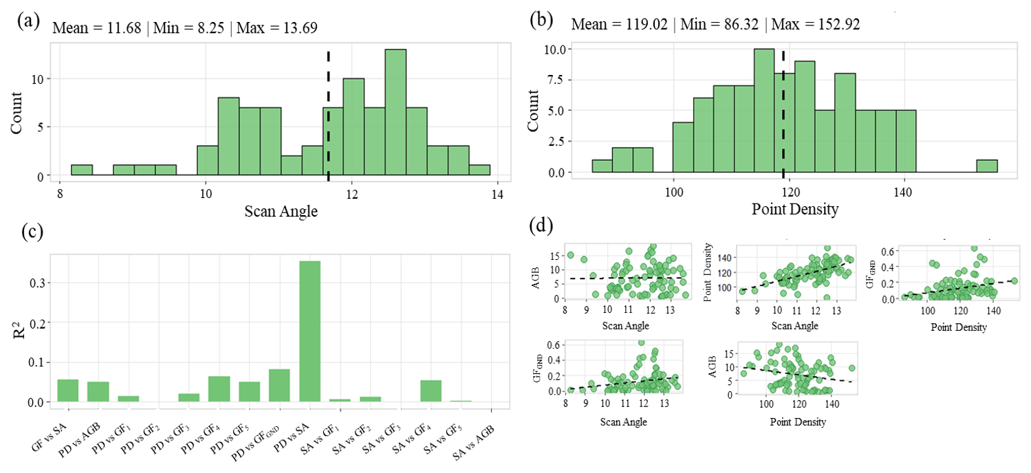
Figure B3 Top panels show the distributions of (a) mean scan angle (SA) and (b) mean LiDAR point density (PD) calculated for all sampling polygons across all acquisition dates. Panel (c) summarizes the coefficients of determination (R²) between SA, PD, destructive AGB, the conventional ground-based gap fraction (GF_GND), and the five 20 cm multi-layer gap fraction layers (GF₁ − GF₅). Panel (d) presents representative scatter plots illustrating the relationships between SA and AGB, SA and PD, PD and GF_GND, SA and GF_GND, and PD and AGB. The consistently weak relationships between SA, PD, AGB, and the LiDAR structural features demonstrate that the selected acquisition parameters (double-grid flight pattern, 50 % overlap, and maximum scan angle of 25°) effectively minimized scan angle and point density effects on the biomass estimation workflow.

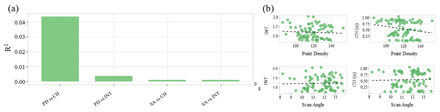
Figure B4 Panel (a) summarizes the coefficients of determination (R²) between point density (PD), scan angle (SA), LiDAR crop height (CH), and normalized LiDAR intensity (INT). Panel (b) presents the corresponding scatter plots for PD versus INT, PD versus CH, SA versus INT, and SA versus CH. The weak relationships observed for both CH and normalized INT indicate that the selected acquisition parameters (double-grid flight pattern, 50 % overlap, and maximum scan angle of 25°) effectively minimized the influence of scan angle and point density on these LiDAR features used for above-ground biomass estimation.

B4 k Adapted 3DPI Parameterization

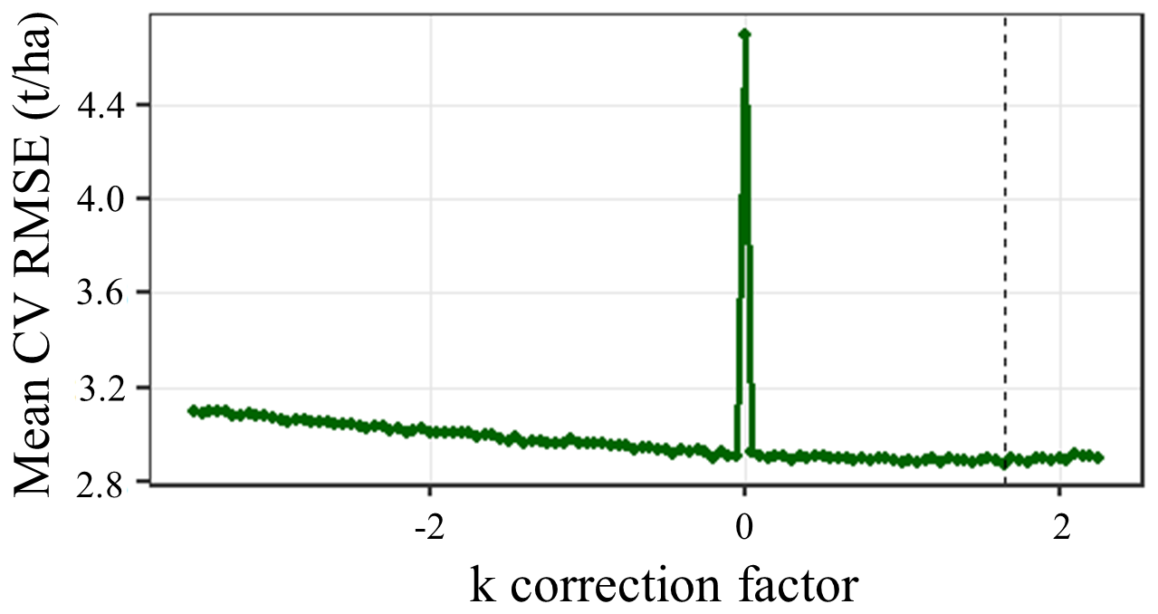
Figure B5 Mean cross-validation RMSE obtained from repeated 10-fold cross-validation for the adapted 3DPI formulation using a range of extinction correction coefficients (k). The optimal coefficient (k=1.65; dashed vertical line) corresponded to the minimum mean RMSE and was subsequently used for all 3DPI analyses presented in this study.

B5 ANN Training and Testing Performance

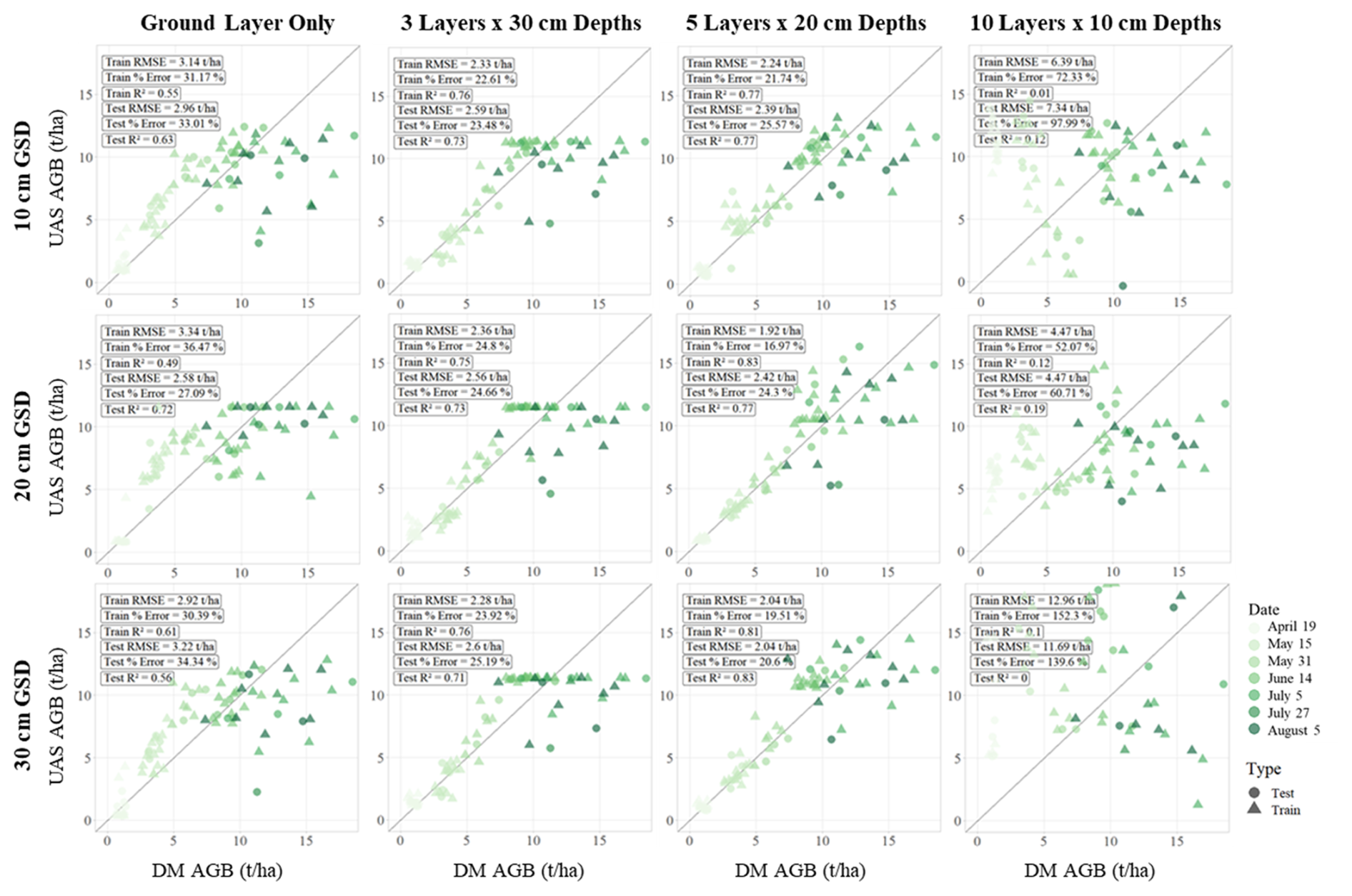
Figure B6 Observed versus predicted above-ground biomass (AGB) for ANN models trained using different LiDAR gap fraction (GF) parameterizations. Columns represent increasing vertical segmentation, ranging from the conventional ground-based gap fraction (GF_GND) to 3×30, 5×20, and 10×10 cm multi-layer GF configurations, while rows represent decreasing horizontal ground sampling distance (GSD) from 30 to 20 and 10 cm. Marker color indicates acquisition date and marker shape distinguishes training and testing samples. Training and testing RMSE, relative error, and R² are reported within each panel. The 5×20 cm GF configuration with a 30 cm GSD achieved the best overall balance between model accuracy and generalization, whereas the finest 10×10 cm segmentation exhibited substantially reduced testing performance, indicating increased sensitivity to sparse point distributions and model overfitting.

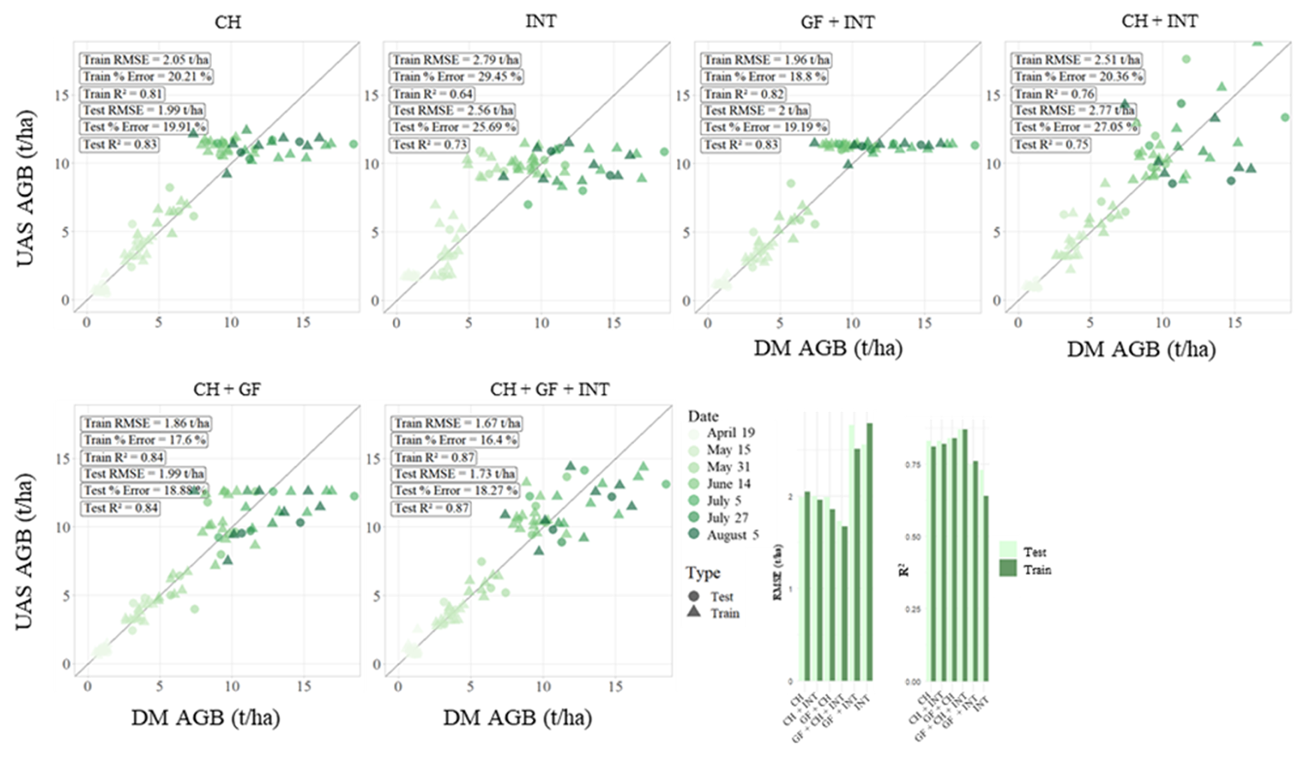
Figure B7 Observed versus predicted above-ground biomass (AGB) for ANN models using different combinations of LiDAR-derived crop height (CH), 5 layer gap fraction (GF) (20 cm layer depth), and field-normalized LiDAR intensity (INT). All models were generated using the optimal 30 cm ground sampling distance (GSD) identified in the GF sensitivity analysis. Marker color indicates acquisition date and marker shape distinguishes training and testing samples. Training and testing RMSE, relative error, and R² are reported within each panel. The accompanying summary plots compare testing RMSE and R² across the evaluated LiDAR feature combinations, illustrating the progressive improvement obtained by incorporating complementary canopy density and normalized intensity information alongside crop height.

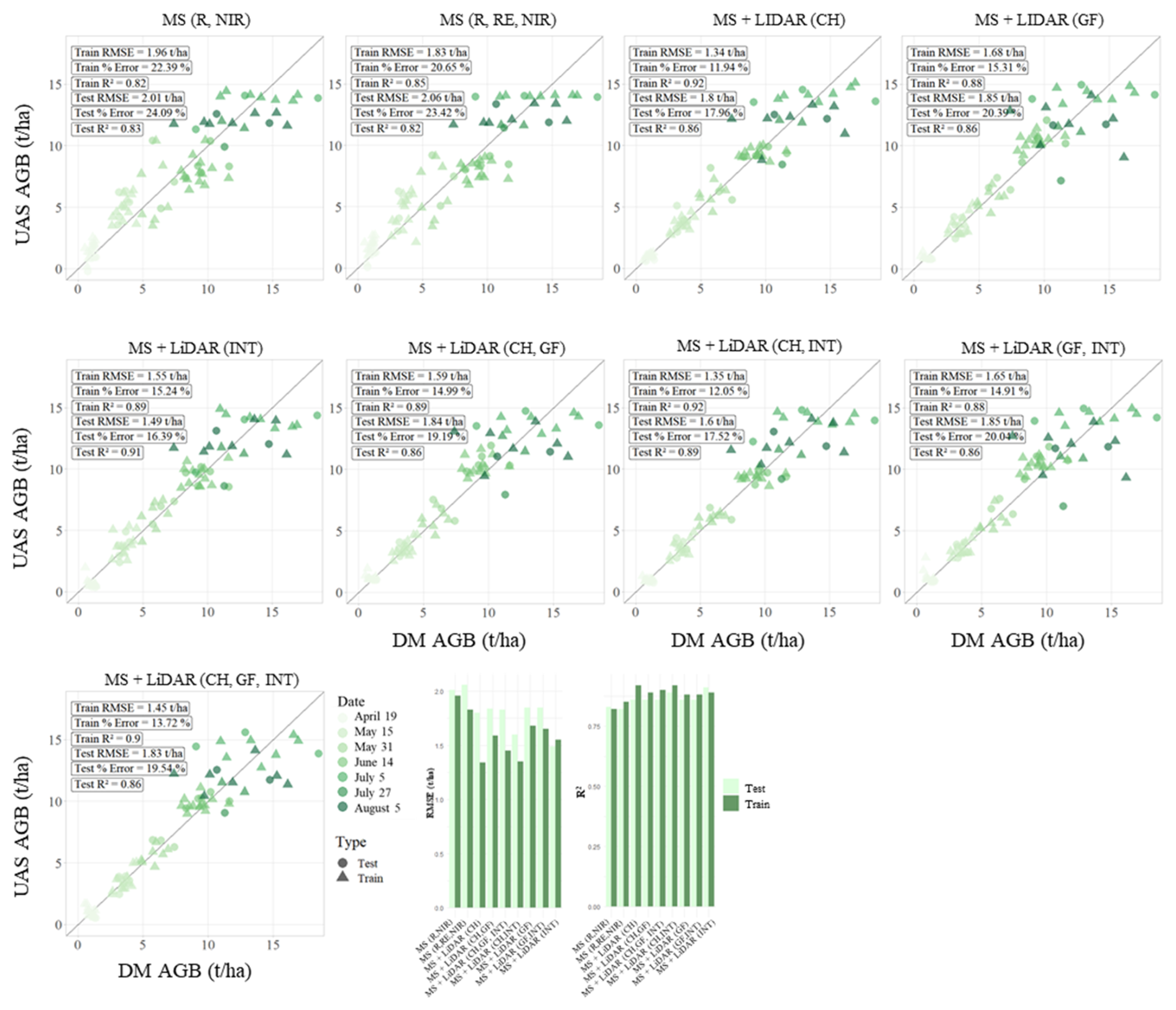
Figure B8 Observed versus predicted above-ground biomass (AGB) for ANN models using multispectral (MS) reflectance (Red, Red-edge, and Near-Infrared (NIR)) individually and in combination with LiDAR-derived crop height (CH), 5 layer gap fraction (GF) (20 cm layer depth), and field-normalized LiDAR intensity (INT). All models were generated using the optimal 30 cm ground sampling distance (GSD) identified in the GF sensitivity analysis. Marker color indicates acquisition date and marker shape distinguishes training and testing samples. Training and testing RMSE, relative error, and R² are reported within each panel. The accompanying summary plots compare testing RMSE and R² across the evaluated feature combinations, illustrating the improvement achieved by integrating multispectral reflectance with complementary LiDAR-derived structural and normalized intensity information.

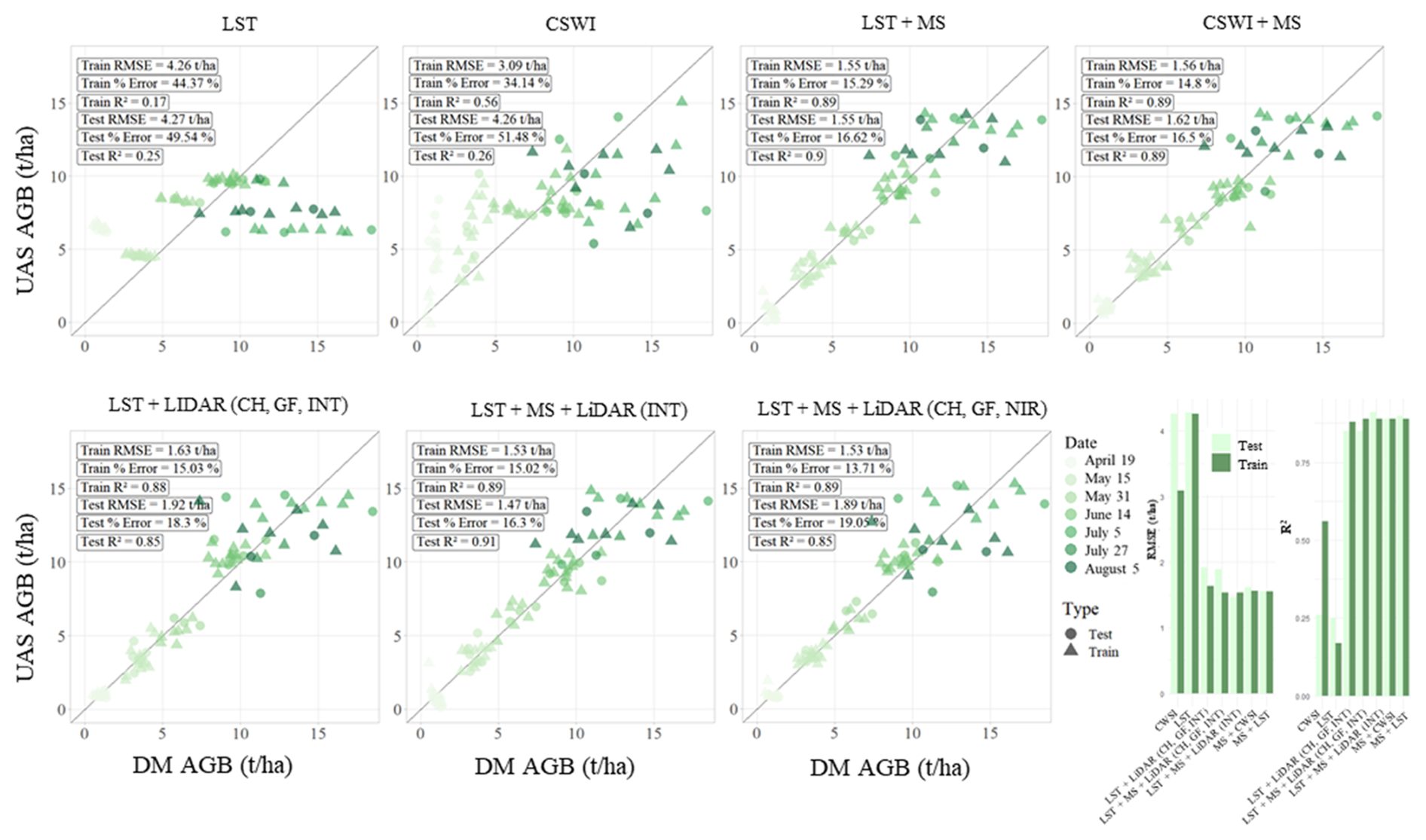
Figure B9 Observed versus predicted above-ground biomass (AGB) for ANN models using thermal infrared (TIR) features, including land surface temperature (LST) and the Crop Water Stress Index (CWSI), individually and in combination with multispectral (MS; Red, Red-edge, and Near-Infrared (NIR)) reflectance and LiDAR-derived crop height (CH), 5 multi-layer gap fraction (GF; 20 cm layer depth), and field-normalized LiDAR intensity (INT). All models were generated using the optimal 30 cm ground sampling distance (GSD) identified in the GF sensitivity analysis. Marker color indicates acquisition date and marker shape distinguishes training and testing samples. Training and testing RMSE, relative error, and R2 are reported within each panel. The accompanying summary plots compare testing RMSE and R² across the evaluated feature combinations, illustrating the limited predictive capability of TIR features alone and their complementary contribution when integrated with multispectral reflectance and LiDAR-derived structural information.

B6 Growth-Stage Performance

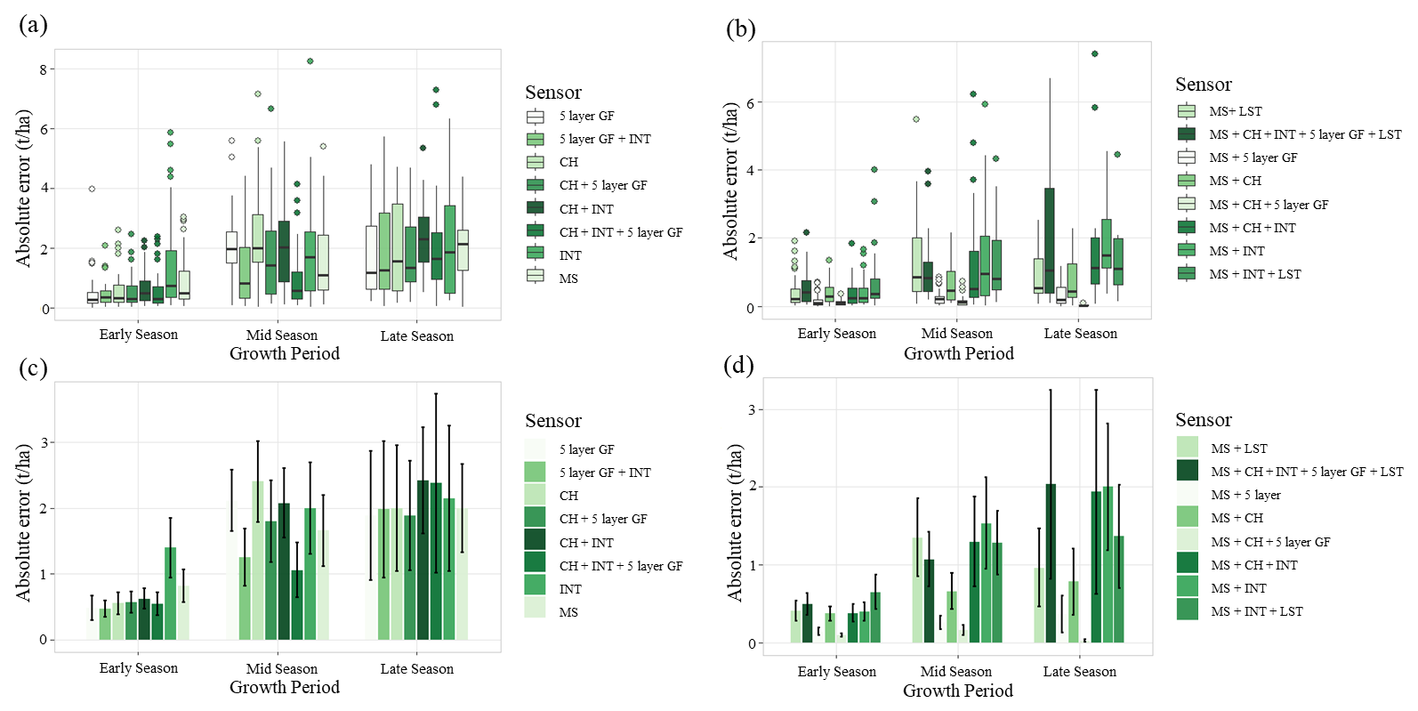
Figure B10 The left panels show the best-performing single-sensor feature combinations, while the right panels show the best-performing multi-sensor fusion models. The top panels present the distribution of absolute prediction errors (t ha⁻¹) as boxplots, and the bottom panels summarize the corresponding mean absolute prediction errors (± SD) for each growth period. Growth periods were defined as early season (19 April–31 May), mid-season (14 June–5 July), and late season (27 July–5 August). These results complement the analyses presented in the main manuscript by illustrating the magnitude and variability of biomass prediction errors throughout crop development and across the evaluated sensor configurations.

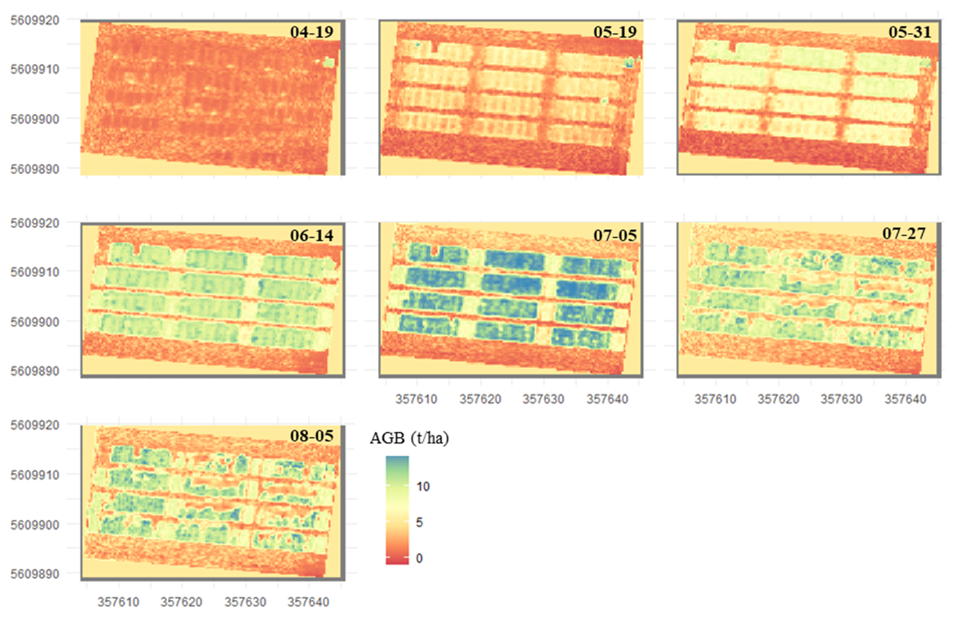
Figure B11 AGB maps generated for each UAV acquisition date using the combined LiDAR-derived crop height (CH), 5 layer gap fraction (GF; 20 cm layer depth), and field-normalized LiDAR intensity (INT) ANN model. Values are displayed on a common color scale (t ha⁻¹), illustrating the temporal progression of spatial variability in biomass accumulation. The high-resolution maps demonstrate the capability of UAV LiDAR features to provide spatially continuous biomass estimates beyond the discrete locations available from destructive sampling.