Asymmetry in carbon cycle feedbacks and transient climate response under positive and negative CO₂ emissions

Most emissions scenarios consistent with limiting warming to well below 2 °C above pre-industrial levels rely on carbon dioxide removal (CDR) to balance residual positive emissions or achieve net-negative emissions. While carbon cycle and climate metrics are well quantified for positive CO₂ emissions, applying the same metrics under negative emissions may over- or underestimate the effectiveness of CDR. This study uses an Earth system model to investigate the asymmetry in carbon cycle feedbacks and the transient climate response under positive and negative CO₂ emissions. To this end, symmetric concentration-driven simulations are initialized from a state at equilibrium with twice the preindustrial CO₂ concentration and run in biogeochemically coupled, radiatively coupled and fully coupled modes. Our results suggest that land and ocean carbon cycle feedbacks are asymmetric. Compared to their respective magnitudes under positive emissions, the concentration-carbon feedback is larger, whereas the climate-carbon feedback is smaller under negative emissions. Asymmetries in land carbon cycle feedbacks arise from the saturation of the CO₂ fertilization effect and asymmetric temperature and soil respiration responses. Asymmetries in ocean carbon cycle feedbacks are driven by non-linear responses to CO₂ and temperature change, as well as asymmetric ocean circulation responses. Asymmetries in carbon cycle feedbacks propagate onto asymmetry in the Transient Climate Response to Cumulative CO₂ Emissions (TCRE): a negative CO₂ emission results in greater global mean temperature change than a CO₂ emission of the same magnitude. Our study highlights the need to quantify metrics under negative emissions as reliance on metrics derived from positive emission scenarios may result in inaccurate quantification of the climate response under net negative CO₂ emissions.

1 Introduction

The potential for dangerous climate impacts due to anthropogenic CO₂ emissions prompted the signing of the Paris Agreement, which seeks to limit global warming to well below 2 °C above pre-industrial levels, and pursue further efforts to limit it to 1.5 °C (UNFCCC, 2015). To achieve either climate goal by year 2100, substantial emissions cuts are required immediately (United Nations Environment Programme, 2020). Emissions scenarios consistent with the Paris Agreement climate goals heavily rely on carbon dioxide removal from the atmosphere (CDR), not only to balance difficult-to-mitigate emissions, but also achieve net-negative emissions, that is, when the amount of CO₂ removed from the atmosphere exceeds the amount of CO₂ added to the atmosphere. Examples of CDR approaches include bioenergy with carbon capture and storage (BECCS), afforestation and reforestation, direct air capture of CO₂ with carbon capture and storage (DACCS), and ocean alkalinity enhancement, among others (Pathak et al., 2022; Smith et al., 2023).

Emissions scenarios consistent with global climate goals are designed with an assumption of symmetry, that is, removals are applied as negative emissions that balance positive emissions, assuming symmetry in climate outcomes (Zickfeld et al., 2021). For this assumption to hold, the carbon cycle and climate response to a positive CO₂ emission needs to be of equal magnitude and opposite sign to its response to a negative CO₂ emission (Zickfeld et al., 2021). Research shows that this asymmetry does not hold for the carbon cycle, and uncertainties exist for the temperature response, particularly with regards to the sign of the asymmetry (Zickfeld et al., 2016, 2021; Canadell et al., 2021; Koven et al., 2022a, b). Therefore, this study aims to investigate the asymmetry in carbon cycle feedbacks and the climate response under positive and negative CO₂ emissions, focusing on two research questions:

1. To what extent are global land carbon cycle feedbacks symmetric and what are the mechanisms that drive possible asymmetry?

2. To what extent is the temperature response – as quantified through the Transient Climate Response to Cumulative CO₂ Emissions or Removals (TCRE and TCRR metrics) – symmetric, and what drives possible asymmetry?

It is worth noting that symmetry as defined here is distinct from reversibility. Reversibility defines the extent to which a climate variable returns to a specified level in a given time period after the forcing is restored. Irreversibility can be caused by the exceedance of a critical threshold that results in a transition to a different stable state, or system inertia, that is, the lag in the response to forcing. Symmetry describes whether the value of a metric or a trajectory mirror each other. Here, asymmetry refers to the difference in a variable or metric after inertia effects have been corrected for. In this case, asymmetry is driven by nonlinearities and state dependencies in the response to forcing.

Carbon cycling on land and in the ocean regulates atmospheric CO₂ concentration under negative emissions, as it does under positive CO₂ emissions. If negative emissions are implemented but removals remain lower than emissions (net-positive emissions), the land and ocean carbon sinks continue to take up carbon, albeit at a lower rate (Tokarska and Zickfeld, 2015; Jones et al., 2016; Melnikova et al. 2021; Koven et al., 2022a). Once the amount of CO₂ removed from the atmosphere exceeds the amount of CO₂ added to the atmosphere (net-negative emissions), the carbon sinks are expected to weaken further and may reverse, counteracting CDR efforts (Cao and Caldeira, 2010; Tokarska and Zickfeld, 2015; Jones et al., 2016; Melnikova et al., 2021; Zickfeld et al., 2021; Canadell et al., 2021; Koven et al., 2022a). Under net-negative emissions, declining atmospheric CO₂ concentration results in a reversal of carbon sinks to sources (negative concentration-carbon feedback), whereas cooling associated with declining atmospheric CO₂ results in CO₂ uptake (positive climate-carbon feedback) (Schwinger and Tjiputra, 2018; Chimuka et al., 2023). The magnitude of these feedbacks determines the extent to which land and ocean carbon cycle responses counteract CDR, and therefore, how effective CDR will be in achieving climate goals (Chimuka et al., 2023).

Quantifying the magnitudes of carbon cycle feedbacks under net-negative emissions, however, is complicated by climate system inertia. The “CDR-reversibility” simulation, which has been commonly used for carbon cycle feedback quantification under negative emissions (Schwinger and Tjiputra, 2018; Melnikova et al., 2021; Chimuka et al., 2023; Asaadi et al., 2024), is characterized by a CO₂ concentration increase at a rate of 1 % yr⁻¹, followed immediately by a ramp-down at the same rate back to preindustrial CO₂ levels (CDR-MIP: Keller et al., 2014). Studies using these simulations show a lagged carbon cycle response in the ramp-down phase because of climate-system inertia: carbon pools respond to both the decreasing CO₂ concentration and prior increasing CO₂ concentration (Tokarska and Zickfeld, 2015; Zickfeld et al., 2016; Schwinger and Tjiputra, 2018). This lagged response results in smaller carbon pool changes, and therefore, smaller magnitudes of feedbacks under net-negative emissions relative to positive emissions (Schwinger and Tjiputra, 2018; Chimuka et al., 2023). Chimuka et al. (2023) proposed a novel approach to address climate system inertia and more accurately quantify carbon cycle feedbacks under net-negative emissions. In this approach, climate system inertia was quantified through zero emissions simulations, then subtracted from the CDR-reversibility simulations to isolate the response to negative emissions alone. Findings showed larger feedbacks under negative emissions in the inertia-corrected approach than in the standard approach due to the reduction of climate system inertia effects.

Asymmetries in carbon cycle feedbacks affect the airborne or removal fraction, and thus, are expected to propagate onto symmetry in the temperature response. The temperature response to CO₂ emissions is commonly quantified by the Transient Climate response to Cumulative CO₂ Emissions (TCRE) – the ratio of the transient global mean warming to cumulative CO₂ emissions (Matthews et al., 2009). The TCRE is approximately constant over time and across scenarios (Matthews et al., 2009; Gillett et al., 2013; Ehlert et al., 2017; Matthews et al., 2017). Studies exploring the TCRE show that the linear relationship still holds under negative emissions if the temperature response is corrected for ocean thermal and carbon cycle inertia effects as quantified by the zero emissions commitment (Zickfeld et al., 2016; Koven et al., 2022a, b; Sanderson et al., 2025). The TCRE under net-negative emissions is also referred to as the transient climate response to cumulative CO₂ removals (TCRR) (Zickfeld et al., 2021). The magnitude of the TCRE and TCRR asymmetry is highly uncertain (Zickfeld et al., 2016, 2021; Canadell et al., 2021; Koven et al., 2022a, b). Furthermore, the sign of the temperature asymmetry varies across models, with some models exhibiting a larger temperature response under positive emissions and others under negative emissions (Canadell et al., 2021; Koven et al., 2022a; Sanderson et al., 2025).

This paper explores the extent to which carbon cycle feedbacks and the transient climate response to CO₂ emissions and removals are asymmetric and the mechanisms behind the asymmetry. Section 2 outlines the experimental design and climate model simulations used as well as the frameworks used to quantify carbon cycle feedback and climate metrics. Section 3 presents the land and ocean carbon cycle feedback and TCRE and TCRR asymmetry results, and the associated mechanisms behind the asymmetry. Understanding the symmetry in carbon cycle feedbacks is integral for determining whether the same metrics, that is, carbon cycle feedback parameters or the TCRE and TCRR, can be applied under both positive and negative emissions.

2 Methods

2.1 Model Description

We use the University of Victoria Earth System Climate Model (UVic ESCM, version 2.10) – a model of intermediate complexity with a horizontal grid resolution of 1.8° (meridional) × 3.6° (zonal) (Weaver et al., 2001; Mengis et al., 2020). The atmosphere model is a 2D energy-moisture balance model with dynamical wind feedbacks. Atmospheric heat and freshwater are transported through diffusion and advection (Weaver et al., 2001), based on wind velocities prescribed from monthly climatological wind fields from NCAR/NCEP reanalysis data (Eby et al., 2013). This simplified atmosphere model is coupled to a 19-layer 3D ocean general circulation model, including ocean inorganic and organic carbon cycle models, and based on the Geophysical Fluid Dynamics Laboratory (GFDL) Modular Ocean Model version 2 (MOM2; Pacanowski, 1995). The coupled dynamic–thermodynamic sea ice model simulates sea ice dynamics through elastic, viscous, and plastic deformation and flow mechanisms (Weaver et al., 2001).

The land surface model, based on the Hadley Centre Met Office Surface Exchange Scheme (MOSES), simulates the terrestrial carbon cycle and is coupled to the Top-Down Representation of Interactive Foliage and Flora including Dynamics (TRIFFID) model which simulates vegetation and soil carbon (Meissner et al., 2003). This model version also includes a permafrost carbon model in the soil module that simulates permafrost carbon through a diffusion-based scheme (MacDougall and Knutti, 2016). Ocean carbon is represented by an inorganic ocean carbon model following the Ocean Carbon Model Intercomparison Protocol (OCMIP), and an NPZD (nutrient, phytoplankton, zooplankton, detritus) model of ocean biology simulating carbon uptake by the biological pump, accounting for phytoplankton light and iron limitations (Keller et al., 2012).

2.2 Model Simulations

The model was first integrated under a CO₂ concentration twice that at preindustrial (∼ 560 ppm) for 6000 years to achieve an equilibrium state. All other greenhouse gas and aerosol forcings, surface land conditions, and orbital parameters were held at 1850 levels according to the Coupled Model Intercomparison Project Phase 6 (CMIP6) experimental design protocol (Eyring et al., 2016). The solar forcing was set to the 1850–1873 mean and the volcanic forcing was held at its average over 1850–2014, also consistent with the CMIP6 protocol (Eyring et al., 2016).

Following the 2 × CO₂ spin-up, two idealized symmetric concentration-driven simulations were run. Concentration-driven simulations were chosen in order to expose the land and ocean to the same CO₂ concentrations, facilitating easier separation of concentration-carbon and climate-carbon feedbacks (Gregory et al., 2009; Zickfeld et al., 2011; Schwinger et al., 2014). Both simulations were initialized from a state of equilibrium to quantify the response to positive and negative emissions without climate system inertia effects. In one simulation, atmospheric CO₂ concentration was prescribed to increase at 1 % yr⁻¹ until three times the preindustrial CO₂ concentration, and in another the atmospheric CO₂ concentration was prescribed to decline back to preindustrial levels, mirroring the trajectory of the 1 % yr⁻¹ CO₂ increase simulation (Fig. 1a). In both simulations, it takes roughly 43 years to reach three times the preindustrial CO₂ concentration and preindustrial respectively. We refer to the simulation with increasing atmospheric CO₂ concentration as the 1 % yr⁻¹ symmetric positive emissions (PE) simulation, and the simulation with decreasing atmospheric CO₂ concentration as the 1 % yr⁻¹ symmetric negative emissions (NE) simulation. Although concentrations are symmetric in both simulations, the diagnosed emissions differ; cumulative positive emissions are approximately 800 Pg C, whereas cumulative negative emissions are 970 Pg C (Fig. 1c). The negative emissions simulation includes substantial levels of negative emissions that cannot be achieved in the real world (Powis et al., 2023). However, this simulation is symmetric with respect to CO₂ concentrations in the positive emissions simulation, allowing for the quantification of asymmetry in climate-carbon cycle response (Fig. 1a).

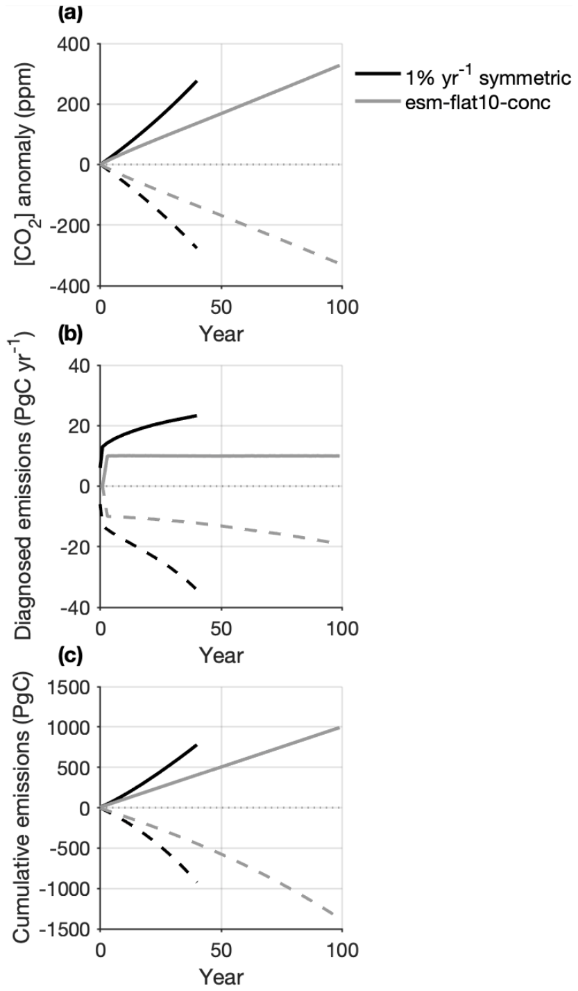
Figure 1 (a) Prescribed atmospheric CO₂ concentration, (b) diagnosed annual positive and negative CO₂ emissions, and (c) diagnosed cumulative positive and negative CO₂ emissions in the fully coupled (FULL) 1 % yr⁻¹ symmetric and esm-flat10-conc positive (PE) and negative (NE) emissions simulations. Solid lines represent the positive emissions run; dashed lines represent the negative emissions run. The rate of CO₂ concentration change in panel (a). is calculated relative to the 2 × CO₂ equilibrium state.

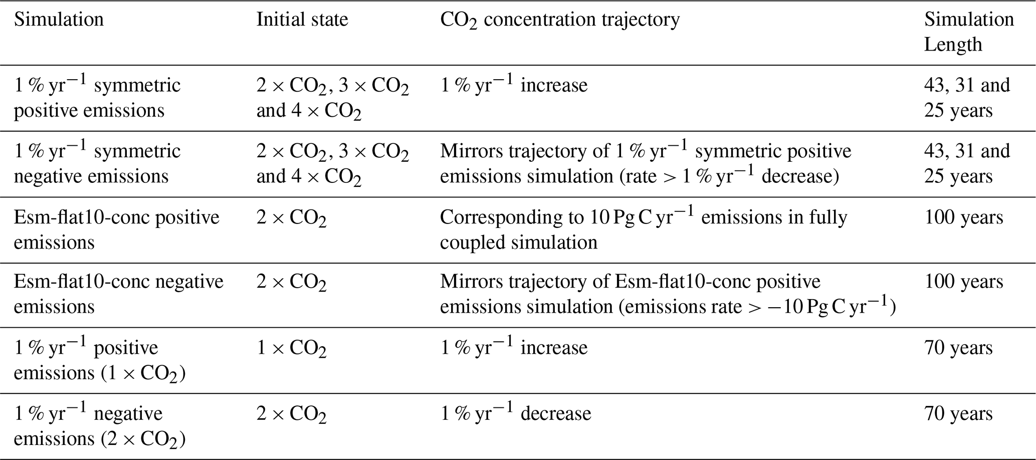
To assess the rate-dependence of the asymmetry in the climate-carbon cycle response to positive and negative emissions, we ran additional symmetric concentration-driven simulations derived from the esm-flat10 simulations by Sanderson et al. (2024, 2025). The esm-flat10 simulations are emissions-driven simulations with a constant emissions rate of 10 Pg C yr⁻¹ for 100 years, reaching cumulative emissions of 1000 Pg C. These simulations were designed in line with current annual CO₂ emissions rates and with the goal of diagnosing climate metrics such as the TCRE. As concentration-driven simulations are best suited for the calculation of feedbacks (Arora et al., 2013), we modified the esm-flat10 simulation as follows: First, a fully coupled emissions-driven esm-flat10 simulation was initialized from the an equilibrium state twice the preindustrial CO₂ concentration, then the CO₂ concentration trajectory from that simulation was used to force a concentration-driven simulation, referred to here as the esm-flat10-conc positive emissions simulation (Fig. 1a). In an additional step, the CO₂ trajectory was mirrored over the x-axis to obtain a symmetric trajectory with declining atmospheric CO₂. This CO₂ trajectory was used to run a second simulation, referred to as the esm-flat10-conc negative emissions simulation (Fig. 1a). The rate-dependence was determined by comparing the magnitude and sign of carbon cycle feedbacks and TCRE asymmetry in the 1 % yr⁻¹ and esm-flat10-conc simulation pairs. We ran the 1 % yr⁻¹ symmetric simulations from 2 additional equilibrium states – three times (3 × CO₂) and four times (4 × CO₂) the preindustrial CO₂ concentration – to test the sensitivity of climate-carbon cycle asymmetry to the initial state (Table 1). Lastly, we ran two additional simulations to explore an alternative experimental design for quantifying carbon cycle feedback and TCRE asymmetry (Fig. S1 in the Supplement, Table 1). In one simulation, atmospheric CO₂ concentration was prescribed to increase at 1 % yr⁻¹ from a preindustrial equilibrium state until two times the preindustrial CO₂ concentration. We refer to this as this as 1 % yr⁻¹ positive emissions (1 × CO₂) simulation. In the second simulation, atmospheric CO₂ concentration was prescribed to decline from a 2 × CO₂ equilibrium state to preindustrial levels at a rate of 1 % yr⁻¹, and refer to this as the 1 % yr⁻¹ negative emissions simulation (2 × CO₂). This experimental design is similar to the 1 % yr⁻¹ ramp up and ramp down simulation used in reversibility studies, except that the Earth System was given time to equilibrate with a doubled pre-industrial atmospheric CO₂ concentration before CO₂ was prescribed to decline. As in our main experimental design, this design allows us to quantify the response to positive and negative emissions without climate system inertia effects, and thus, we can compare the results between the two experimental designs. All simulations used in this study are briefly described in Table 1.

Table 1 Overview of simulations used in this study. Note that the initial state refers to the equilibrium state from which the simulation was initialized. All simulations were run in concentration-driven configuration.

All simulations were run in three modes, following the C4MIP protocol for the quantification of carbon cycle feedbacks (Friedlingstein et al., 2006; Arora et al., 2013, 2020; Jones et al., 2016):

• Fully coupled mode (FULL): the entire Earth system responds to the specified change in atmospheric CO₂ concentration or CO₂ emissions – in this mode, the land and ocean carbon sinks are subject to changing atmospheric CO₂ concentration and temperature.

• Biogeochemically coupled mode (BGC): the land and ocean carbon sinks are subject to changing atmospheric CO₂ concentration but not changing temperature – this is achieved by prescribing a specified time-invariant CO₂ concentration to the radiation module (the CO₂ concentration of the respective equilibrium state from which the simulation was initialized), while the land and ocean carbon cycle modules see an evolving atmospheric CO₂ concentration.

• Radiatively coupled mode (RAD): the land and ocean carbon sinks are subject to changes in temperature but no change in atmospheric CO₂ concentration – the land and ocean carbon cycle modules see a specified time invariant CO₂ concentration (the CO₂ concentration of the respective equilibrium state from which the simulation was initialized), while the radiation module sees changing atmospheric CO₂ concentration.

Non-CO₂ forcings, including forcings due to other greenhouse gases and aerosols, were held fixed at their preindustrial values.

2.3 Metric Quantification

Asymmetry in global carbon cycle feedbacks was determined by comparing the magnitudes and signs of feedback parameters under positive and negative emissions, evaluated at the end of the 1 % yr⁻¹ symmetric simulations. Feedback parameters were quantified following the integrated flux-based feedback framework from Friedlingstein et al. (2006) (see Sect. 2.3.1 below). Feedback parameters under negative emissions were also compared to those from Chimuka et al. (2023), where they were quantified including climate system inertia effects and then corrected for that inertia. The carbon cycle feedback parameters in the remaining 4 simulations were computed at the same atmospheric CO₂ concentration change, that is, when atmospheric CO₂ concentration change reached 280 ppm relative to the spin-up, for ease of comparison to the feedback parameters in the 1 % yr⁻¹ symmetric simulations.

The temperature asymmetry was assessed in two ways: (1) using a framework that approximates the TCRE and TCRR utilizing the Jones and Friedlingstein (2020) framework and (2) using the direct calculation of the TCRE and TCRR metrics, in which the TCRE was computed as the temperature change for a given amount of cumulative CO₂ emissions, and the TCRR as the temperature change for a given amount of cumulative CO₂ removals. Since the simulations used are concentration-driven, diagnosed emissions were used for the direct calculation of the TCRE and TCRR. The Jones and Friedlingstein (2020) framework uses the global carbon cycle feedback parameters and the transient climate sensitivity metric from the fully coupled modes to approximate the TCRE and TCRR (see Sect. 2.3.2 below). For validation purposes, the metrics computed from this method were then compared to those calculated using the direct calculation, evaluated at the end of the simulation. The TCRE and TCRR metrics for all simulations were computed at the cumulative emissions level in the 1 % yr⁻¹ symmetric positive emissions simulation. The temperature asymmetry was then determined by comparing the magnitudes of the TCRE and TCRR metrics.

2.3.1 Global Carbon Cycle Feedback Framework

Carbon cycle feedbacks were quantified using integrated flux-based feedback parameters (Friedlingstein et al., 2006). In the Friedlingstein et al. (2006) feedback framework, the change in land (ocean) carbon due to both CO₂ and climate changes is expressed as the linear sum of the land (ocean) response to the change in the atmospheric CO₂ concentration ΔC_A and surface air temperature ΔT:

$$\begin{array}{}\text{(1)}& {\displaystyle }\mathrm{\Delta }{C}_{\mathrm{L}}={\mathit{\beta }}_{\mathrm{L}}\mathrm{\Delta }{C}_{\mathrm{A}}+{\mathit{\gamma }}_{\mathrm{L}}\mathrm{\Delta }T\text{(2)}& {\displaystyle }\mathrm{\Delta }{C}_{\mathrm{O}}={\mathit{\beta }}_{\mathrm{O}}\mathrm{\Delta }{C}_{\mathrm{A}}+{\mathit{\gamma }}_{\mathrm{O}}\mathrm{\Delta }T\end{array}$$

The concentration-carbon feedback parameter (β) quantifies the carbon cycle response to changes in CO₂ concentration in units of Pg C ppm⁻¹, whereas the climate-carbon feedback parameter (γ) quantifies the carbon cycle response to changes in temperature in units of Pg C °C⁻¹ (Friedlingstein et al., 2006). The change in land and ocean carbon due to the increasing atmospheric CO₂ concentration alone is determined using the biogeochemically coupled simulation. In this simulation, the land and ocean only respond to changes in CO₂ concentration, and therefore, this simulation can be used to quantify the concentration-carbon feedback (Friedlingstein et al., 2006). Warming is still observed in this simulation because the water use efficiency of vegetation increases at higher CO₂ concentrations, and changes in albedo, due to shifts in vegetation structure and spatial distribution, result in a small warming effect (Cox et al., 2004; Boer and Arora, 2013; Arora et al., 2013). However, this warming is considered negligible in this feedback framework (Friedlingstein et al., 2006; Arora et al., 2020; Asaadi et al., 2024). Assuming ΔT = 0 in Eqs. (1) and (2), the change in land and ocean carbon is given as:

$$\begin{array}{}\text{(3a)}& {\displaystyle }\mathrm{\Delta }{C}_{\mathrm{L}}={\mathit{\beta }}_{\mathrm{L}}\mathrm{\Delta }{C}_{\mathrm{A}}\text{(4a)}& {\displaystyle }\mathrm{\Delta }{C}_{\mathrm{O}}={\mathit{\beta }}_{\mathrm{O}}\mathrm{\Delta }{C}_{\mathrm{A}}\end{array}$$

Equations (3a) and (4a) can then be rearranged to solve for the concentration-carbon feedback parameter β as follows:

$$\begin{array}{}\text{(3b)}& {\displaystyle }{\mathit{\beta }}_{\mathrm{L}}={\displaystyle \frac{\mathrm{\Delta }{C}_{\mathrm{L}}}{\mathrm{\Delta }{C}_{\mathrm{A}}}}\text{(4b)}& {\displaystyle }{\mathit{\beta }}_{\mathrm{O}}={\displaystyle \frac{\mathrm{\Delta }{C}_{\mathrm{O}}}{\mathrm{\Delta }{C}_{\mathrm{A}}}}\end{array}$$

The change in land (ocean) carbon due to climate alone is determined using the radiatively coupled simulation. In this simulation, the land and ocean only respond to changes in climate, and therefore, this simulation can be used to quantify the climate-carbon feedback (Friedlingstein et al., 2006). The change in land and ocean carbon is expressed as:

$$\begin{array}{}\text{(5a)}& {\displaystyle }\mathrm{\Delta }{C}_{\mathrm{L}}={\mathit{\gamma }}_{\mathrm{L}}\mathrm{\Delta }T\text{(6a)}& {\displaystyle }\mathrm{\Delta }{C}_{\mathrm{O}}={\mathit{\gamma }}_{\mathrm{O}}\mathrm{\Delta }T\end{array}$$

Equations (5a) and (6a) can then be rearranged to solve for the climate-carbon feedback parameter γ as follows:

$$\begin{array}{}\text{(5b)}& {\displaystyle }{\mathit{\gamma }}_{\mathrm{L}}={\displaystyle \frac{\mathrm{\Delta }{C}_{\mathrm{L}}}{\mathrm{\Delta }T}}\text{(6b)}& {\displaystyle }{\mathit{\gamma }}_{\mathrm{O}}={\displaystyle \frac{\mathrm{\Delta }{C}_{\mathrm{O}}}{\mathrm{\Delta }T}}\end{array}$$

An alternative method for quantifying the change in land (ocean) carbon due to climate change uses the fully coupled and biogeochemically coupled simulations (Arora et al., 2013). We refer to this method as the FULL-BGC method. Here, the change in land (ocean) carbon in the biogeochemically coupled simulation (BGC) is subtracted from that in the fully coupled simulation (FULL) and expressed as the product of the climate-carbon feedback parameter, and the difference between the surface air temperature changes in the two simulations:

$$\begin{array}{}\text{(7a)}& {\displaystyle }\mathrm{\Delta }{C}_{\mathrm{L}}^{\mathrm{FULL}}-\mathrm{\Delta }{C}_{\mathrm{L}}^{\mathrm{BGC}}={\mathit{\gamma }}_{\mathrm{L}}\left(\mathrm{\Delta }{T}^{\mathrm{FULL}}-\mathrm{\Delta }{T}^{\mathrm{BGC}}\right)\text{(8a)}& {\displaystyle }\mathrm{\Delta }{C}_{\mathrm{O}}^{\mathrm{FULL}}-\mathrm{\Delta }{C}_{\mathrm{O}}^{\mathrm{BGC}}={\mathit{\gamma }}_{\mathrm{O}}\left(\mathrm{\Delta }{T}^{\mathrm{FULL}}-\mathrm{\Delta }{T}^{\mathrm{BGC}}\right)\end{array}$$

Assuming ΔT = 0 here as well, Eqs. (7a) and (8a) can then be rearranged to solve for the climate-carbon feedback parameter γ as follows:

$$\begin{array}{}\text{(7b)}& {\displaystyle }{\mathit{\gamma }}_{\mathrm{L}}={\displaystyle \frac{\mathrm{\Delta }{C}_{\mathrm{L}}^{\mathrm{FULL}}-\mathrm{\Delta }{C}_{\mathrm{L}}^{\mathrm{BGC}}}{\mathrm{\Delta }{T}^{\mathrm{FULL}}}}\text{(8b)}& {\displaystyle }{\mathit{\gamma }}_{\mathrm{O}}={\displaystyle \frac{\mathrm{\Delta }{C}_{\mathrm{O}}^{\mathrm{FULL}}-\mathrm{\Delta }{C}_{\mathrm{O}}^{\mathrm{BGC}}}{\mathrm{\Delta }{T}^{\mathrm{FULL}}}}\end{array}$$

Feedback parameters were evaluated from Eqs. (3)–(6) for the positive and negative emissions simulations.

2.3.2 Decomposition of Land Concentration-carbon Feedback Parameter

To better understand the processes driving the asymmetry in the concentration-carbon feedback, we used a framework that decomposes β into vegetation and soil carbon, and the underlying processes, as described in Arora et al. (2020):

$$\begin{array}{}\text{(9)}& \begin{array}{rl}{\mathit{\beta }}_{\mathrm{L}}=& {\displaystyle \frac{\mathrm{\Delta }{C}_{\mathrm{L}}^{\mathrm{BGC}}}{\mathrm{\Delta }{C}_{\mathrm{A}}}}={\displaystyle \frac{\mathrm{\Delta }{C}_{\mathrm{V}}^{\mathrm{BGC}}+\mathrm{\Delta }{C}_{\mathrm{S}}^{\mathrm{BGC}}}{\mathrm{\Delta }{C}_{\mathrm{A}}}}\\ =& \left({\displaystyle \frac{\mathrm{\Delta }{C}_{\mathrm{V}}^{\mathrm{BGC}}}{\mathrm{\Delta }{\mathrm{NPP}}^{\mathrm{BGC}}}}{\displaystyle \frac{\mathrm{\Delta }{\mathrm{NPP}}^{\mathrm{BGC}}}{\mathrm{\Delta }{\mathrm{GPP}}^{\mathrm{BGC}}}}{\displaystyle \frac{\mathrm{\Delta }{\mathrm{GPP}}^{\mathrm{BGC}}}{\mathrm{\Delta }{C}_{\mathrm{A}}}}\right)\\ & +\left({\displaystyle \frac{\mathrm{\Delta }{C}_{\mathrm{S}}^{\mathrm{BGC}}}{\mathrm{\Delta }{R}_{\mathrm{h}}^{\mathrm{BGC}}}}{\displaystyle \frac{\mathrm{\Delta }{R}_{\mathrm{h}}^{\mathrm{BGC}}}{\mathrm{\Delta }{\mathrm{LF}}^{\mathrm{BGC}}}}{\displaystyle \frac{\mathrm{\Delta }{\mathrm{LF}}^{\mathrm{BGC}}}{\mathrm{\Delta }{C}_{\mathrm{A}}}}\right)\\ =& {\mathit{\tau }}_{\mathrm{cveg}\mathrm{\Delta }}{\mathrm{CUE}}_{\mathrm{\Delta }}{\displaystyle \frac{\mathrm{\Delta }{\mathrm{GPP}}^{\mathrm{BGC}}}{\mathrm{\Delta }{C}_{\mathrm{A}}}}\\ & +{\mathit{\tau }}_{\mathrm{csoil}\mathrm{\Delta }}{\displaystyle \frac{\mathrm{\Delta }{R}_{\mathrm{h}}^{\mathrm{BGC}}}{\mathrm{\Delta }{\mathrm{LF}}^{\mathrm{BGC}}}}{\displaystyle \frac{\mathrm{\Delta }{\mathrm{LF}}^{\mathrm{BGC}}}{\mathrm{\Delta }{C}_{\mathrm{A}}}}\end{array}\end{array}$$

The sensitivity of vegetation carbon to changes in CO₂ concentration can be decomposed to a product of the residence time of vegetation carbon τ_cvegΔ, the carbon use efficiency (CUE) – proportion of GPP that is turned into NPP – and a measure of the CO₂ fertilization effect. The sensitivity of soil carbon to changes in CO₂ concentration can be decomposed to a product of the residence time of soil carbon τ_csoilΔ, the change in the soil respiration rate per unit change in the leaf litter flux, and the sensitivity of the leaf litter flux to changes in CO₂ concentration. All changes in variables were calculated relative to the equilibrium state from the simulations were initialized. The relative contribution of each term to the asymmetry in the concentration-carbon feedback can be determined by taking the first derivative of Eq. (9) (Sect. S1.1). The percentage contribution of each term was then computed and included in Sect. 3.2.2 and Table S1.

2.3.3 Transient Climate Response to Cumulative CO₂ Emissions (TCRE) Framework

The Transient Climate Response to Cumulative CO₂ Emissions (TCRE) is a near-linear relationship between transient warming and cumulative CO₂ emissions (Matthews et al., 2009). According to the Jones and Friedlingstein (2020) framework, the TCRE can be expressed as the product of the climate sensitivity parameter (α) and the cumulative airborne fraction (AF) as follows:

$$\begin{array}{}\text{(10)}& \mathrm{TCRE}=\mathit{\alpha }\left({\displaystyle \frac{\mathrm{AF}}{k}}\right)\end{array}$$

where k is a constant to account for unit conversion (k = 2.12 Pg C ppm⁻¹).

The cumulative airborne fraction can be expressed in a form with individual carbon cycle feedback parameters as follows:

$$\begin{array}{}\text{(11)}& \mathrm{AF}={\displaystyle \frac{k}{k+\mathit{\beta }+\mathit{\alpha }\mathit{\gamma }}}\end{array}$$

Substituting Eq. (11) into Eq. (10) gives the TCRE as:

$$\begin{array}{}\text{(12)}& \mathrm{TCRE}={\displaystyle \frac{\mathit{\alpha }}{k+\mathit{\beta }+\mathit{\alpha }\mathit{\gamma }}}\end{array}$$

To explore the relative contribution of the asymmetry in the climate sensitivity parameter, airborne fraction and carbon cycle feedbacks to the asymmetry in the TCRE, the first derivative of Eq. (12) (Sect. S1.2 in the Supplement) was computed and used to determine the contribution of the asymmetry in each variable to the asymmetry in the TCRE (Sect. 3.3).

2.3.4 Determining the sign of asymmetry

As aforementioned, all metrics were computed under positive and negative emissions and compared to determine the magnitude and sign of asymmetry. The asymmetry was determined as follows:

$$\begin{array}{}\text{(13)}& \mathrm{asymmetry}=X_{\mathrm{neg}}-X_{\mathrm{pos}}\end{array}$$

where “X” denotes β_L, β_O, γ_L, γ_O, TCRE or TCRR under positive (“pos”) or negative (“neg”) emissions. Therefore, the asymmetry is positive (negative) when a given metric is larger (smaller) under negative emissions.

3 Results

Our results section focuses on carbon cycle feedback and TCRE asymmetry under positive and negative emissions. Section 3.1–3.2 explore the carbon cycle feedback asymmetry from the 1 % yr⁻¹ simulation pairs, and the rate- and state-dependence of these results. Section 3.3 focuses on TCRE asymmetry and its rate- and state-dependence and Sect. 3.4 explores results using an alternative experimental design.

3.1 Physical Climate Response

The prescribed atmospheric CO₂ concentration profiles in the 1 % yr⁻¹ symmetric simulations are symmetric by design, with a change in CO₂ concentration of ∼ 280 ppm (Fig. 2a). However, the surface air temperature shows considerable asymmetry in the FULL and RAD modes (Fig. 2b). In both modes, the surface air temperature decreases more in the negative emissions simulation relative to the positive emissions simulation by approximately 0.5 °C (Fig. 2b). This occurs because of the approximately logarithmic relationship between radiative forcing and atmospheric CO₂ concentration, which leads to a greater response to declining than rising CO₂ levels (Myre et al., 2001; Eby et al., 2013; Etminan et al., 2016). The BGC mode for both simulations exhibits small temperature changes (Fig. 2a, b) that result from biophysical responses to changes in CO₂ concentration, such as changes in the evapotranspiration flux and surface albedo (Cox et al., 2004; Boer and Arora, 2013; Arora et al., 2013). The difference between the FULL and RAD temperature responses is also due to these biophysical responses.

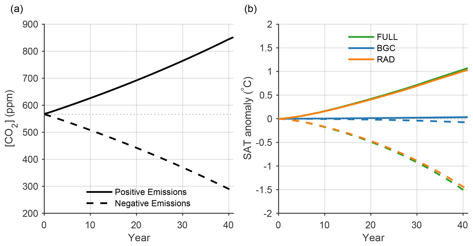
Figure 2 (a) Prescribed atmospheric CO₂ concentration and (b) surface air temperature (SAT) change in the fully coupled (FULL), biogeochemically coupled (BGC) and radiatively coupled (RAD) 1 % yr⁻¹ symmetric positive (PE) and negative (NE) emissions simulations relative to the 2 × CO₂ equilibrium state.

3.2 Quantifying Carbon Cycle Feedback Asymmetry

3.2.1 Land Carbon Change Asymmetry in the FULL Mode

Despite symmetry in the atmospheric CO₂ concentration profiles in Fig. 2a, the land carbon pool exhibits asymmetry for all 3 modes (Fig. 3a). Asymmetry in carbon pools is determined by comparing the carbon change at the end of the 1 % yr⁻¹ symmetric positive and negative emissions. If the carbon change is greater under negative (positive) emissions, then the asymmetry is positive (negative) (see Sect. 2.3.4). The FULL mode exhibits the greatest asymmetry of all 3 modes, with the land gaining 70.7 Pg C under positive emissions and losing 154 Pg C under negative emissions (Fig. 3a). This results in a positive asymmetry of roughly 83 Pg C. The sign of the asymmetry is the same for both vegetation and soil carbon pools, with the vegetation carbon pool exhibiting the larger positive asymmetry (PE: 35.3 Pg C; NE: −90.5 Pg C) (Fig. 3c, d).

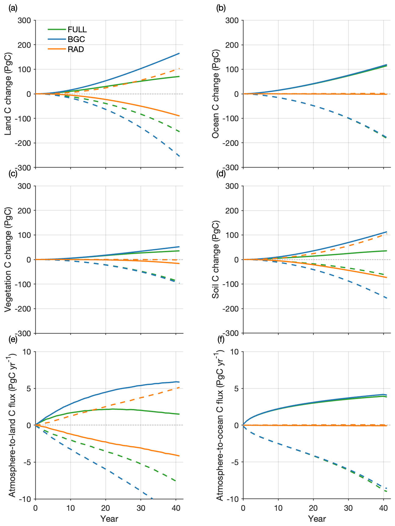
Figure 3 (a) Land, (b) ocean, (c) vegetation and (d) soil carbon pool changes as a function of time for the fully coupled (FULL), biogeochemically coupled (BGC) and radiatively coupled (RAD) modes of the 1 % yr⁻¹ symmetric positive and negative emissions simulations. Solid lines represent the positive emissions run; dashed lines represent the negative emissions run. Panels (a)–(d) are calculated relative to the 2 × CO₂ equilibrium state. The atmospheric carbon fluxes are also shown in panels (e) and (f).

The land carbon flux balance determines the change in the land carbon pool. Under positive emissions, the CO₂ fertilization effect drives carbon uptake; photosynthesis is enhanced under increasing CO₂ concentration, increasing NPP (Fig. 4a). Warming enhances soil respiration, but the soil respiration remains lower than NPP, leading to land carbon sequestration. Under negative emissions, NPP is consistently lower than soil respiration largely because of the asymmetry in NPP under increasing and declining CO₂ concentrations (Fig. 4a). The saturation of NPP at higher atmospheric CO₂ concentration results in a smaller enhancement of NPP with increasing CO₂ concentration and a larger reduction in NPP with decreasing CO₂ concentration. Soil respiration is also asymmetric: with cooling decreasing soil respiration more than warming increases soil respiration (Fig. 4a), consistent with the asymmetric temperature response in the FULL mode (Fig. 2b). As NPP decreases faster than soil respiration under negative emissions, the land loses CO₂ to the atmosphere.

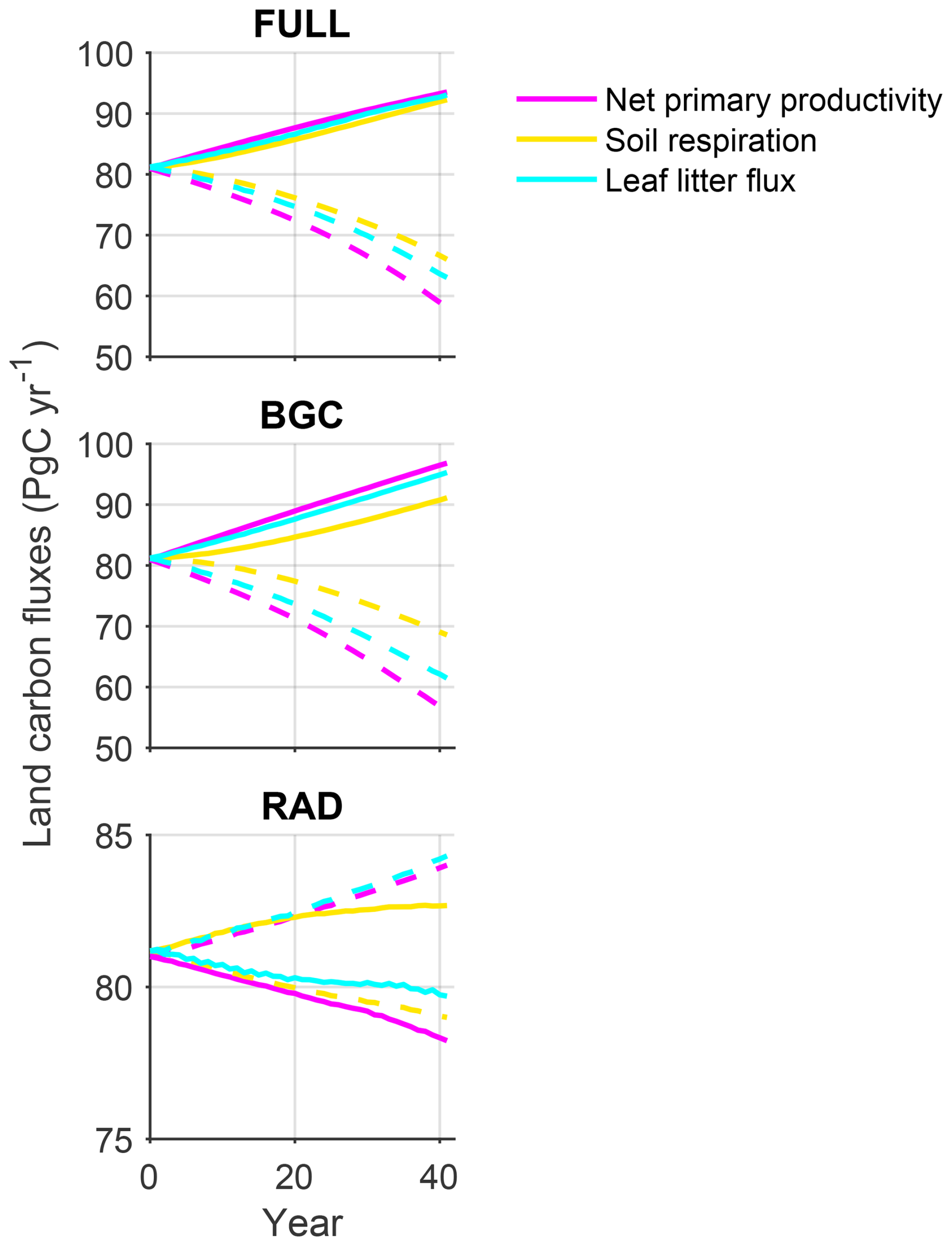
Figure 4 Land carbon fluxes for the three modes of the 1 % yr⁻¹ symmetric simulations are shown. NPP = net primary productivity, LLF = leaf litter flux and SR = soil respiration. Fully coupled (FULL); biogeochemically coupled (BGC); radiatively coupled (RAD). Solid lines represent the positive (PE) emissions run; dashed lines represent the negative emissions (NE) run. Note the difference in the vertical scale of the RAD panel (last panel).

3.2.2 Land Carbon Change Asymmetry in the BGC Mode

Isolating the component of the land carbon response due to changes in atmospheric CO₂ concentration only (BGC mode), our results consistently show asymmetry in land carbon change (Fig. 3a). In the 1 % yr⁻¹ symmetric positive emissions simulation, the land carbon pool gains about 165 Pg C, whereas it loses 255 Pg C in the negative emissions simulation (Fig. 3a). This results in a positive asymmetry of 90 Pg C. The sign and magnitude of the asymmetry is similar for the vegetation and soil carbon pools (positive asymmetry of approximately 50 Pg C) (Fig. 3c, d).

Similar to the FULL mode, the strengthening of the CO₂ fertilization effect promotes carbon uptake under positive emissions and carbon loss under negative emissions as the CO₂ fertilization effect weakens (Fig. 4b). The vegetation and soil carbon components of the response to CO₂ (Fig. 4c, d) can each be decomposed into three terms according to Arora et al. (2020) to better understand the mechanisms driving the observed asymmetries (Eq. 9). Of the vegetation-related terms, the greatest contributors to the asymmetry in the concentration-carbon feedback are increased sensitivity of NPP to CO₂ concentration change (36 %) and longer vegetation carbon residence time under negative emissions (15 %) (Table S1). The response of the litter flux to changes in CO₂ concentration is the greatest contributor to the asymmetry in the land response to CO₂ (45 %). The asymmetry in the soil respiration flux response to changes in leaf litter input is negative, and thus, this terms reduces the asymmetry of the concentration-carbon feedback (−15 %) (Table S1).

3.2.3 Land Carbon Change Asymmetry in the RAD Mode

Through the RAD mode, which shows the land carbon response to climate change, our results show the least asymmetry of all three modes (Fig. 3a). The land loses 90.1 Pg C in the 1 % yr⁻¹ symmetric positive emissions simulation and gains 103 Pg C in the negative emissions simulation, resulting in a positive asymmetry of 12.9 Pg C (Fig. 3a). The sign of the asymmetry in the soil carbon pool is consistent with that for the land carbon pool, with the soil carbon pool losing 73.7 Pg C under positive emissions and gaining 105.1 Pg C under negative emissions (Fig. 3d). The asymmetry in the vegetation carbon pool, however, is small and negative (Fig. 3c) and by the end of the simulation, the vegetation carbon pools in both simulations lose carbon (PE: −1.8 Pg C; NE: −16.4 Pg C) (Fig. 3c).

In the absence of the CO₂ fertilization effect, NPP declines with warming, primarily due to an increase in plant respiration, while soil respiration increases with warming under positive emissions. As soil respiration is greater than NPP, the land releases CO₂ into the atmosphere (Fig. 4c). Under negative emissions, NPP increases as plant respiration decreases with cooling, whereas, soil respiration declines (Fig. 4c). NPP remains greater than soil respiration, promoting carbon sequestration.

3.2.4 Ocean Carbon Change Asymmetry in the FULL, BGC and RAD modes

The ocean carbon pool exhibits considerable positive asymmetry in the FULL and BGC modes (Fig. 3b), losing more carbon in the 1 % yr⁻¹ symmetric negative emissions simulation than it gains in the positive emissions simulation, consistent with previous literature (Zickfeld et al., 2021). If the carbon change is greater under negative (positive) emissions, then the asymmetry is positive (negative) (see Sect. 2.3.4). The magnitude of the positive asymmetry is similar for the FULL and BGC modes, whereas the RAD mode shows small negative asymmetry (PE: −2 Pg C; NE: 1.7 Pg C) (Fig. 3b).

In the FULL mode, the overall response to CO₂ and temperature changes combined results in a larger flux of CO₂ out of the ocean under negative emissions than the flux into the ocean under positive emissions (Fig. 3f) (Zickfeld et al., 2021). This asymmetric ocean carbon response is partly driven by the imbalance between atmospheric CO₂ concentration and the partial pressure of CO₂ in the surface ocean, which results in a larger flux of CO₂ out of the ocean under negative emissions than the flux into the ocean under positive emissions (Fig. 3f, see Fig. S2). There is a non-linear inverse relationship between the ocean's ability to buffer additional CO₂ and the partial pressure of CO₂ in the surface ocean (Chapin and Eviner, 2014). With increasing partial pressure of CO₂ in the surface ocean, the buffer capacity is expected to decline less than it increases with decreasing partial pressure of CO₂. This relationship favours a greater loss of ocean carbon under negative emissions than gain under positive emissions. Non-linearities related to ocean circulation and CO₂ solubility in seawater also drive the observed ocean carbon asymmetry (Schwinger et al., 2014; Zickfeld et al., 2021). The Atlantic meridional overturning circulation (AMOC) strengthens more under negative emissions than it weakens under positive emissions. Under positive emissions, a weaker AMOC drives less carbon into the ocean due to weaker vertical mixing. Under negative emissions, a stronger AMOC drives a larger flux out of the ocean as carbon is more efficiently mixed upwards and released to the atmosphere (see Fig. S3). The combined effect of the CO₂ concentration imbalance at the atmosphere-ocean interface and the AMOC changes is partly counteracted by the effect of CO₂ solubility changes. The response of CO₂ solubility to changes in ocean temperature is non-linear (Duan and Sun, 2003), that is, the solubility of CO₂ in the surface ocean increases more with cooling than it decreases with warming, resulting in a greater enhancement of carbon uptake capacity under negative emissions than reduction under positive emissions.

The ocean carbon cycle response to CO₂ and temperature changes is isolated in the BGC and RAD modes respectively. In the BGC mode, the imbalance between atmospheric CO₂ concentration and the partial pressure of CO₂ in the surface ocean partly determines the magnitude and direction of the atmosphere-ocean CO₂ flux. This imbalance is larger under negative emissions, resulting in a larger flux of CO₂ out of the ocean under negative emissions than the flux into the ocean under positive emissions (Fig. 3f, see Fig. S2). Non-linearities in buffer capacity (Chapin and Eviner, 2014) also favour greater loss of greater loss of ocean carbon under negative emissions than gain under positive emissions from the ocean's surface, as in the FULL mode. In the RAD mode, the flux out of the ocean under positive emissions is only slightly larger than that into the ocean under negative emissions (Fig. 3f) because of two counteracting effects. The AMOC strengthens more under negative emissions than it weakens under positive emissions, driving a larger flux out of the ocean under negative emissions than the flux into the ocean under positive emissions (see Fig. S3). The effect of AMOC changes is dominated slightly by the non-linearity in the response of CO₂ solubility to changes in ocean temperature (Duan and Sun, 2003): the solubility of CO₂ in the surface ocean increases more with cooling than it decreases with warming, increasing the carbon uptake capacity of the ocean under negative emissions more than it reduces it under positive emissions.

3.2.5 Asymmetry in carbon cycle feedback parameters

The land and ocean carbon response to atmospheric CO₂ concentration gives rise to the negative concentration-carbon feedback: increasing atmospheric CO₂ concentration promotes land and ocean carbon uptake, acting to draw down CO₂ from the atmosphere, whereas declining CO₂ concentration reverses both carbon sinks, releasing CO₂ to the atmosphere. On the other hand, the land and ocean carbon response to temperature change give rise to the positive climate-carbon feedback, in which warming causes land and ocean carbon loss, while cooling promotes carbon gain. The concentration-carbon feedback parameter (β) is quantified from the BGC mode as the land or ocean carbon change per unit change in atmospheric CO₂ concentration (units: Pg C ppm⁻¹). The climate-carbon feedback (γ), computed from the RAD mode, quantifies the land or ocean carbon change per unit change in surface air temperature (units: Pg C °C⁻¹). These feedbacks were quantified using the carbon cycle feedback framework in Sect. 2.3.1 and are shown in Fig. 5.

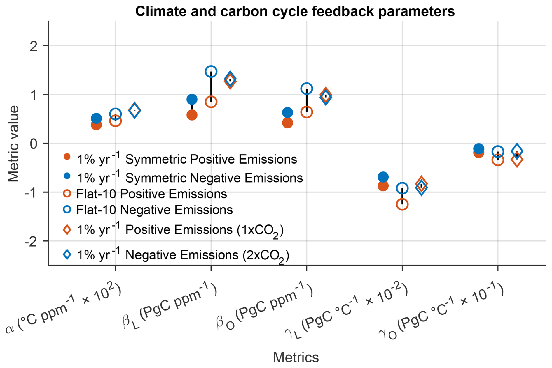
Figure 5 Climate and carbon cycle feedback parameters quantified at a CO₂ concentration change of 280 ppm in all simulations. Feedback parameters under negative emissions are positive for land or ocean carbon loss and negative for land or ocean carbon gain, opposite to the sign convention for feedbacks under positive emissions. Note that the γ_O values are scaled up by one order of magnitude and the γ_L values are scaled up by two orders of magnitude to plot them on the same axis as the β values. Carbon cycle feedback parameters are quantified in units of Pg of carbon per unit ppm and Pg of carbon per unit °C.

Carbon cycle feedback parameters differ in the symmetric 1 % yr⁻¹ positive and negative emissions simulations. The land and ocean β are larger under negative emissions than under positive emissions. Conversely, the land and ocean γ are larger under positive emissions. The asymmetry in γ is partly influenced by the asymmetric temperature response. As the land (ocean) carbon changes in the RAD simulations are comparable, the difference in gamma arises from the magnitude of the temperature change. A larger temperature change under negative emissions means a greater denominator in the gamma calculation (Sect. 2.3.1), favouring a smaller γ under negative emissions. This is only slightly countered by the small positive asymmetry in the land and ocean carbon pools, which favours a larger γ under negative emissions.

3.2.6 Rate- and state-dependence of asymmetry in carbon cycle feedback parameters

The rate-dependence of carbon cycle feedback parameter asymmetry is determined by comparing feedback parameters calculated with the 1 % yr⁻¹ symmetric simulations with those calculated using the esm-flat10-conc simulations. In the esm-flat10-conc positive and negative emissions simulations, CO₂ concentrations evolve at a lower rate, reaching 3 × CO₂ and preindustrial respectively roughly 40 years after the 1 % yr⁻¹ simulations (Fig. 1a). Our results show that both feedbacks are smaller at higher rates of CO₂ change consistent with previous research (Gregory et al., 2009) (Fig. 5). In addition, the magnitude of the asymmetry exhibits rate-dependence: the higher the rate of CO₂ change, the smaller the asymmetry. The sign of the asymmetry, however, is robust. The land and ocean β are larger under negative emissions whereas, land and ocean γ are larger under positive emissions, independent of rate.

In addition to rate-dependence, we investigated whether carbon cycle feedback parameter asymmetry is sensitive to the initial state (Fig. S4). Using 1 % yr⁻¹ symmetric positive and negative emissions simulations initialized from 2 × CO₂, 3 × CO₂ and 4 × CO₂ equilibrium states, we found that for land and ocean β, the magnitude of the asymmetry decreased with increasing initial CO₂ concentration, while the sign of the asymmetry showed no sensitivity to initial state. Findings for land and ocean γ were more complex: although the sign is insensitive to initial state, the magnitude of the asymmetry shows no clear or consistent pattern (Fig. S4).

3.3 Quantifying TCRE asymmetry

In this section, we explore how the asymmetry in carbon cycle feedbacks propagates onto asymmetry in the Transient Climate Response to Cumulative CO₂ Emissions and Removals (TCRE and TCRR) using the fully coupled modes of the 1 % yr⁻¹ symmetric and esm-flat10-conc simulation pairs. Before quantifying TCRE asymmetry, we verified that the global mean temperature change to cumulative emissions relationship for a 2 × CO₂ initial state is linear and only slightly path-dependent (Fig. S5) such that the TCRE is well defined. We quantify this asymmetry using the Jones and Friedlingstein (2020) framework (see Sect. 2.3.1). For validation purposes, we compare this to the direct TCRE and TCRR calculations ($\mathrm{\Delta }T/\mathrm{CE}$ and $\mathrm{\Delta }T/\mathrm{CR}$), where ΔT is the surface air temperature anomaly and CE (CR) is cumulative emissions (removals). Figure 6a shows that the Jones and Friedlingstein (2020) framework generally approximates the TCRE reasonably well in the 1 % yr⁻¹ symmetric positive and negative emissions, especially towards the end of the simulation.

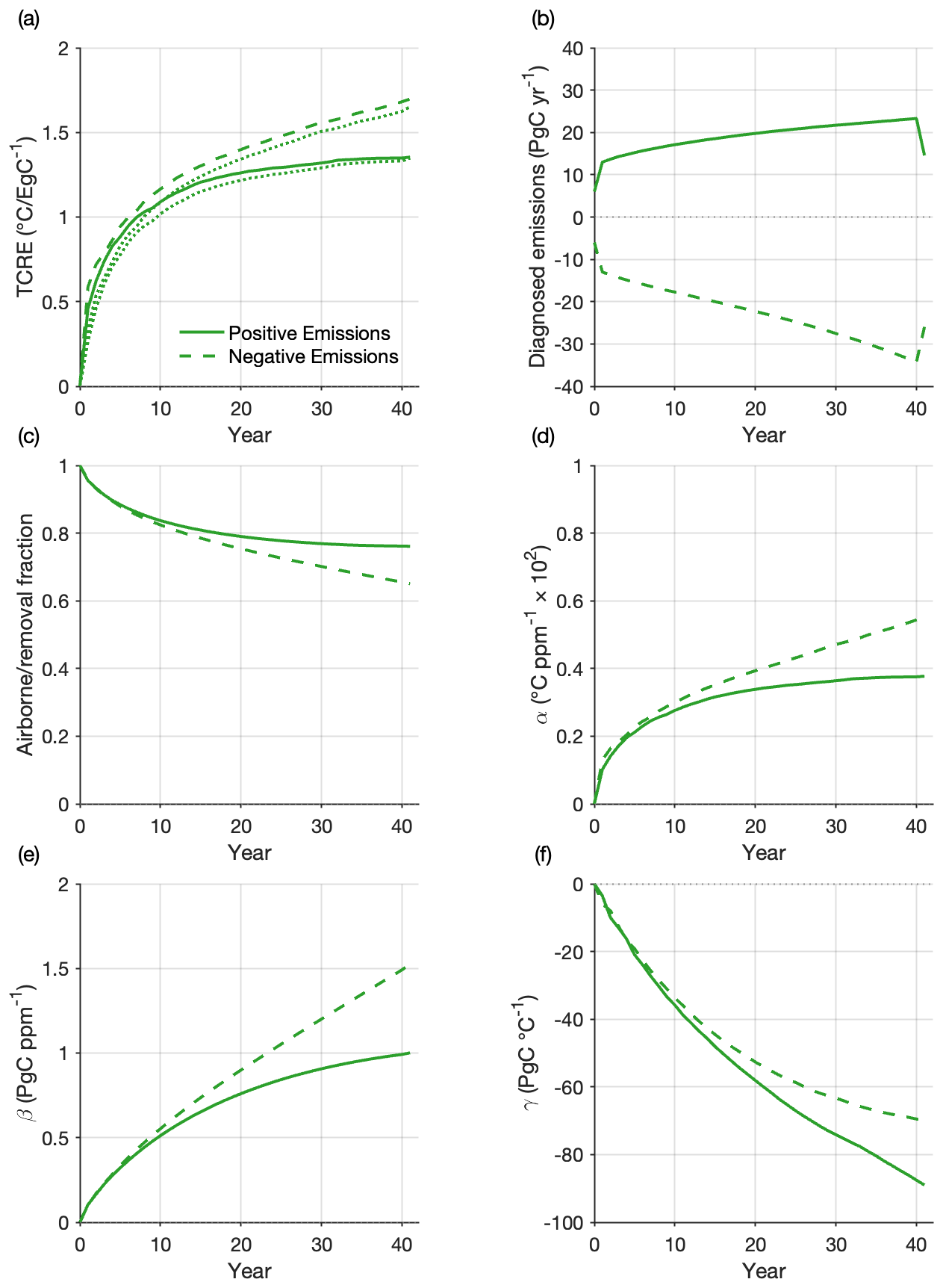
Figure 6 (a) Transient climate response to cumulative CO₂ emissions and removals. Solid and dashed lines – calculated from the Jones and Friedlingstein (2020) framework for the 1 % yr⁻¹ symmetric positive (PE) and negative emissions (NE) runs respectively; dotted lines – direct calculation (ratio of global mean temperature change to cumulative emissions or removals); (b) diagnosed positive or negative emissions; (c) airborne fraction for positive emissions; removal fraction for negative emissions; (d) climate sensitivity parameter α; (e) concentration-carbon feedback parameter β; (f) climate-carbon feedback parameter γ under positive and negative emissions. The TCRE and TCRR are quantified in °C per Eg of carbon, and carbon cycle feedback parameters are quantified in units of Pg of carbon per unit ppm and Pg of carbon per unit °C. The carbon cycle feedbacks represent the total sensitivity of the carbon pools (land plus ocean carbon) to changes in CO₂ concentration and temperature.

The TCRE and TCRR exhibit asymmetry: the cooling per unit negative emission is larger than the warming per unit positive emission (Fig. 6a). The asymmetry in the TCRE is positive, with the TCRE larger in the 1 % yr⁻¹ symmetric negative emissions simulation (1.63 °C EgC⁻¹) than the TCRE in the positive emissions simulation (1.35 °C EgC⁻¹), consistent with Zickfeld et al. (2021). The Jones and Friedlingstein (2020) framework allows us to decompose the TCRE and TCRR into three contributing factors – the airborne or removal fraction (AF $/$ RF), the climate sensitivity (α), and the carbon cycle feedback parameters (β,γ), (see Sect. 2.3.2) – and quantify the asymmetry in each to determine the process driving TCRE asymmetry. The airborne fraction (AF) is defined as the fraction of total emissions that remain in the atmosphere, whereas, the removal fraction (RF) shows the fraction of total removals that stay out of the atmosphere. The removal fraction and airborne fraction are initially equal, then the removal fraction decreases at a greater rate than the airborne fraction until it is smaller by 0.11 (Fig. 6c). The asymmetry in the airborne and removal fractions is negative because diagnosed negative emissions are larger than diagnosed positive emissions (Fig. 6b).

Climate sensitivity (α), a measure of the transient temperature response to changing CO₂ concentration increases at a greater rate under negative emissions, resulting in an asymmetry of 0.0017 °C ppm⁻¹ (Fig. 6d). This positive asymmetry occurs because the surface air temperature anomaly is larger under negative emissions (Fig. 2b). Under negative emissions, a smaller removal fraction favours a smaller TCRR, whereas a larger α favours a larger TCRE. Here, the TCRR is larger in the negative emissions simulation (Fig. 6a), implying that α is the dominant influence on the sign of the TCRE asymmetry.

The airborne and removal fractions can also be computed using α and the two carbon cycle feedback parameters β and γ (see Sect. 2.3.1) (Jones and Friedlingstein, 2020). A larger β acts to reduce the airborne fraction (removal fraction) through land and ocean carbon uptake (loss), a larger γ acts to increase the airborne fraction (removal fraction) through land and ocean carbon loss (uptake). β increases at a greater rate under negative emissions, and by the end of the simulation, the asymmetry is positive, with a β of 1.6 Pg C ppm⁻¹ in the negative emissions simulation and 1.03 Pg C ppm⁻¹ in the positive emissions simulation (Fig. 6e). A larger β acts to reduce the TCRE, favouring a smaller TCRR in the negative emissions simulation. γ decreases faster under positive emissions, and by the end of the simulation, γ is 21 Pg C °C⁻¹ larger in magnitude (negative asymmetry) (Fig. 6f). This occurs because of both larger combined land and ocean carbon loss and surface air temperature change in the negative emissions simulation. A larger γ (in magnitude) favours a larger TCRE in the positive emissions simulation. As aforementioned, α is the key control on the sign of the TCRE asymmetry. The dominant control on the magnitude of the TCRE asymmetry is the positive asymmetry in α. In fact, α is the only contributor that favours positive TCRE asymmetry. The asymmetries in β and γ both favour negative TCRE asymmetry (Sect. S1.2).

Rate- and state-dependence of TCRE asymmetry

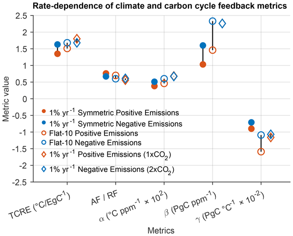
The TCRE asymmetry analysis was repeated with esm-flat10-conc simulations to test the rate-dependence of TCRE asymmetry. The magnitude and sign of the TCRE asymmetry are broadly consistent with results in the 1 % yr⁻¹ symmetric simulations: the sign of the TCRE asymmetry is robust, with the magnitude exhibiting little rate-dependence (Fig. 7). Out of the three contributors to TCRE asymmetry, the carbon cycle feedbacks show the greatest rate-dependence. As described in Sect. 3.1.6, the sign of the asymmetry in feedbacks parameters is robust, whereas the magnitude of the asymmetry in carbon cycle feedback parameters is smaller with higher rates of CO₂ change. An additional insight from Fig. 7 is the relatively large asymmetry observed in β compared to the asymmetry in the TCRE. According to the Jones and Friedlingstein (2020) framework (Sect. 2.3.3), the effect of β on the TCRE counteracts the combined effects of α and γ. The TCRE asymmetry is, therefore, small because of partial cancellation of asymmetry in these contributors.

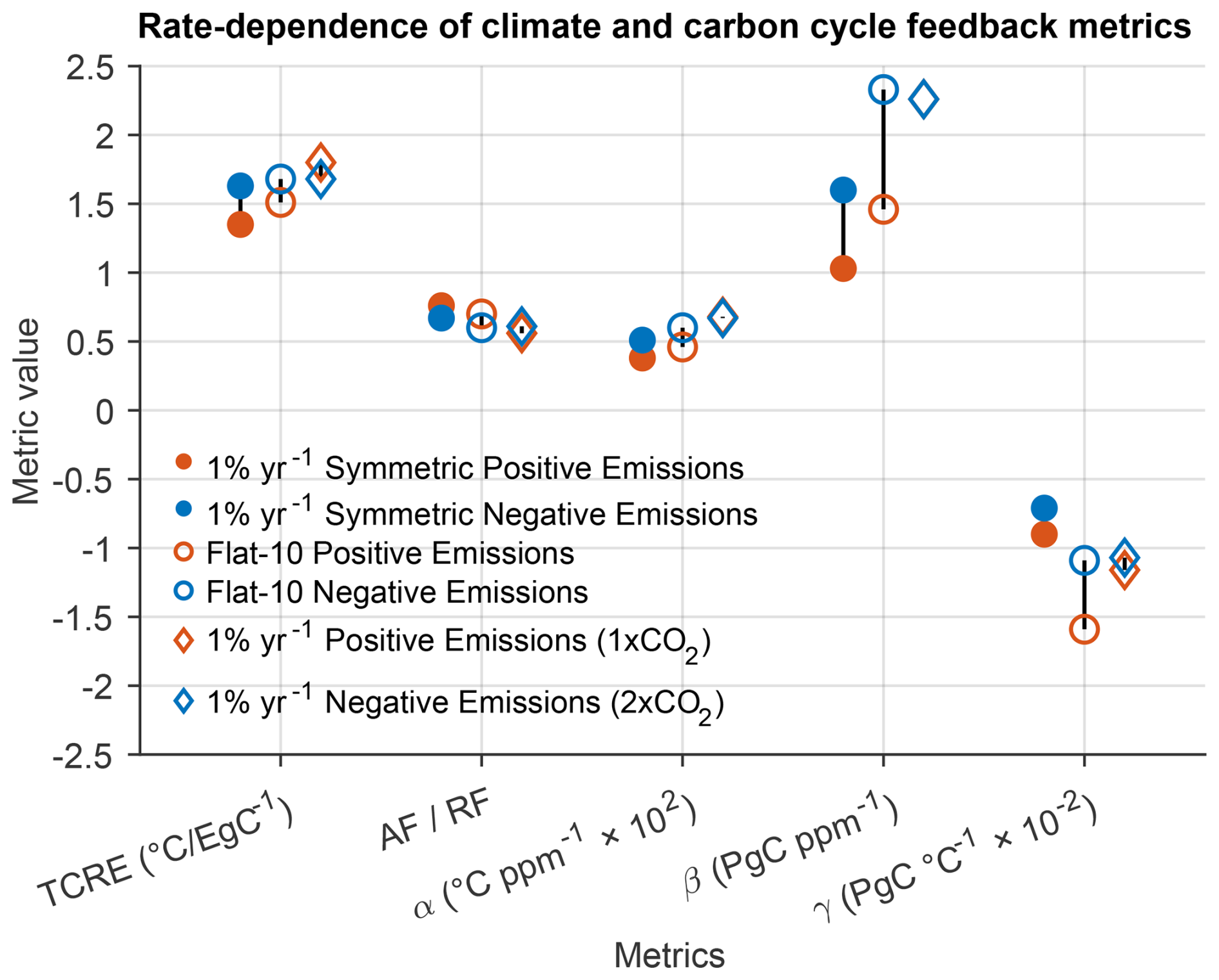
Figure 7 Rate-dependence of climate and carbon cycle feedback metrics in all simulations. Metrics shown include: the transient climate response to cumulative CO₂ emissions and removals (TCRE and TCRR), airborne fraction for positive emissions (AF) and removal fraction for negative emissions (RF), climate sensitivity parameter α, concentration-carbon feedback parameter β and climate-carbon feedback parameter γ. Carbon cycle feedback parameters are quantified in units of Pg of carbon per unit ppm and Pg of carbon per unit °C. The carbon cycle feedbacks represent the total sensitivity of the carbon pools (land plus ocean carbon) to changes in CO₂ concentration and temperature. Vertical black lines depict the asymmetry under positive and negative emissions.

In addition to rate-dependence, we investigated the state-dependence of the TCRE using the 1 % yr⁻¹ symmetry simulations initialized from the 2 × CO₂, 3 × CO₂ and 4 × CO₂ equilibrium states (Fig. S6). The sign of the TCRE asymmetry is state independent, while the magnitude of the asymmetry exhibits little state-dependence, decreasing with higher initial states. Overall, the sign of the TCRE asymmetry is independent of rate and initial state. The magnitude of the asymmetry shows little rate- and state-dependence, increasing with higher rates and decreasing with higher initial states.

3.4 Quantifying Carbon Cycle Feedback and TCRE Asymmetry under Positive and Negative Emissions Applied from Different Equilibrium States

Negative emissions will likely be applied from a state with higher atmospheric CO₂ concentrations than the state positive emissions were applied from. Previous studies have explored carbon cycle feedbacks for this case using the CDR-reversibility simulation and found that the carbon cycle response to negative emissions is contaminated by inertia in response to prior positive emissions (Chimuka et al., 2023). Comparing the ramp-up phase of the CDR-reversibility simulation, which we refer to as the 1 % yr⁻¹ positive emissions simulation (1 × CO₂) (Fig. 1), and the 1 % yr⁻¹ symmetric negative emissions simulation in this study, excludes said climate system inertia effects. Under such a comparison, we find that feedback parameters are smaller under negative emissions and both the carbon cycle feedback and TCRE asymmetry are generally larger than in the experimental design with positive and negative emissions applied form the same 2 × CO₂ state (Figs. 5, 7). It is worth noting that the rate of CO₂ concentration change differs between these simulations (Fig. 1 and Table 1). Thus, we propose a more rate-consistent experimental design using a 1 % yr⁻¹ ramp-down from a 2 × CO₂ state (1 % yr⁻¹ negative emissions simulations (2 × CO₂); see Table 1). Using the two 1 % yr⁻¹ positive and negative emissions simulations, we find larger land feedback parameters and smaller ocean feedback parameters under negative emissions, and the magnitude of carbon cycle feedback asymmetry is smaller than in our 1 % yr⁻¹ symmetric experimental design discussed previously. The magnitude of the TCRE asymmetry is also smaller in the 1 % yr⁻¹ simulations, but the sign reverses. Overall, the magnitude of the asymmetry of the carbon cycle feedback and TCRE asymmetry is smaller due to smaller temperature asymmetry in the 1 % yr⁻¹ simulation pair and different ranges of CO₂ concentrations in the two simulations pairs.

4 Discussion

Carbon cycle feedbacks under negative emissions have previously been quantified from CDR reversibility simulations (CDR-MIP: Keller et al., 2014), in which a phase of CO₂ decline (negative emissions) immediately follows a phase of CO₂ increase (positive emissions). In these studies, the magnitudes of both feedbacks are smaller under negative emissions because of climate system inertia (Schwinger and Tjiputra, 2018; Chimuka et al., 2023). Although other studies using preindustrial as the reference year for quantifying feedbacks under negative emissions show that both feedbacks become larger under negative emissions, they also show the same lagged carbon pool response (Melnikova et al., 2021; Asaadi et al., 2024). Chimuka et al. (2023) proposed an approach to correct for climate system inertia using zero emissions simulations. Compared to the experimental design used here, there is a difference in the initial state, the range of CO₂ concentration, configuration of simulations, and linearity assumptions, and these differences have various implications. First, feedbacks are smaller under positive emissions here than in Chimuka et al. (2023) because the initial CO₂ concentration is higher. At a higher CO₂ level, the sinks are more saturated, and therefore, the sink sensitivity to changes in CO₂ concentration and the temperature response to a given CO₂ concentration are both smaller. Second, although the CO₂ concentration change in both frameworks is the same (∼ 280 ppm), carbon fluxes and pools exhibit different magnitudes of asymmetry due to different ranges of CO₂ concentration in the two frameworks. In this study, the two symmetric simulations span CO₂ concentrations between 2 × CO₂ to 1 × CO₂ and 2 × CO₂ to 3 × CO₂, whereas, in Chimuka et al. (2023), the range of CO₂ concentrations is between 1 × CO₂ and 2 × CO₂. As a result, the two frameworks show different magnitudes of temperature asymmetry and non-linearities in net primary productivity, soil respiration, buffer capacity and the solubility pump impact carbon cycle symmetry.

After correcting for inertia, Chimuka et al. (2023) found a larger climate-carbon feedback and smaller concentration-carbon feedback under negative emissions, whereas we find a smaller climate-carbon feedback and larger concentration-carbon feedbacks under negative emissions. The two studies imply opposite signs of asymmetry due to comparison to different magnitudes of feedbacks under positive emissions, that is, feedbacks under positive emissions are smaller here due to the higher initial state. Furthermore, when feedbacks are compared to those from the ramp-up phase of the CDR-reversibility simulation (as in Sect. 3.4), results are more consistent with Chimuka et al. (2023): we find larger land feedbacks parameters and smaller ocean feedback parameters under negative emissions. Despite discrepancies in the sign of asymmetry, our results are qualitatively consistent with Chimuka et al. (2023): feedbacks under negative emissions are larger in our approach than in the standard CDR-reversibility approach. Feedbacks under negative emissions are generally smaller in this study than those in Chimuka et al. (2023) due to limitations in the correction approach applied in the latter, which is related to linearity assumptions, irreversible vegetation shifts and different simulation configurations (concentration-driven CDR-reversibility simulations and emissions-driven zero emissions simulations) (Chimuka et al., 2023). The benefit of the novel approach used in this study is that it eliminates climate system inertia by prescribing both CO₂ trajectories from the same equilibrium state, allowing for a more accurate quantification of carbon cycle feedbacks under positive and negative emissions.

The temperature response in the FULL mode, as quantified by the TCRE, is asymmetric: the TCRR is larger under negative emissions than the TCRE is under positive emissions, consistent with a previous study that used simulations with symmetric emissions trajectories (Zickfeld et al., 2021). The sign of the temperature asymmetry is generally uncertain in the literature; some models exhibit positive asymmetry (consistent with our findings here) while others exhibit negative asymmetry (Zickfeld et al., 2016; Canadell et al., 2021; Zickfeld et al., 2021; Koven et al., 2022a). The three contributing factors to the TCRE – the airborne or removal fraction (AF $/$ RF), the climate sensitivity (α), and the carbon cycle feedback parameters (β,γ) – are also all asymmetric. Under negative emissions, the removal fraction is smaller than the airborne fraction, favouring a smaller TCRR under negative emissions. However, α is larger under negative emissions, favouring a larger TCRR under negative emissions. Given that the TCRR is larger under negative emissions, this shows that α is the more dominant influence on the sign of the TCRE asymmetry than the airborne and removal fraction are. α also dominates the magnitude of the TCRE asymmetry, followed by β then γ. Overall, carbon cycle feedback asymmetry favours more carbon loss per negative emission than carbon gain per positive emission, whereas, temperature asymmetry favours more cooling per negative emission than warming per positive emission, countering carbon cycle feedback asymmetry.

In the real world, a decline in CO₂ concentration is expected to follow a transient state of positive or zero emissions, rather than an equilibrium state. In this case, carbon cycle feedbacks and the TCRE would be asymmetric with smaller metrics under negative emissions as shown through the CDR-reversibility simulations in earlier studies (Zickfeld et al., 2016; Chimuka et al., 2023). However, the benefit of the experimental design we propose here is that there are no climate system inertia effects (both simulations are prescribed from the same equilibrium state), allowing for a positive and negative emissions to be applied from equilibrium. We chose to initialize our simulations from equilibrium, with the 2 × CO₂ equilibrium state used as default, rather than real world conditions. Findings show that the sign of the concentration-carbon feedback is robust, with the magnitude showing little state-dependence. However, the magnitude of the climate-carbon feedback asymmetry exhibits state-dependence, showing an inconsistent pattern. Our results also suggest that the signs of the carbon cycle feedback and TCRE asymmetries are independent of rate, with only the magnitude of the carbon cycle feedback asymmetry exhibiting notable rate-dependence. The TCRE asymmetry exhibits little state-dependence, and the sign of the asymmetry is robust. These findings align with previous research that carbon-cycle feedbacks exhibit state- and scenario-dependence (Gregory et al., 2009; Boer and Arora, 2010; Zickfeld et al., 2011; Hajima et al., 2014), while the TCRE itself remains largely invariant (Matthews et al., 2009).

The model used here (UVic ESCM) couples the climate and carbon cycles, allowing for the computation of carbon cycle feedbacks, and can run climate model simulations at low computational cost. However, the atmospheric model is a simple energy-moisture balance model, and therefore, is missing several key physical feedbacks such as the cloud feedback and lapse rate feedback, among others. Inclusion of these feedbacks would benefit our TCRE analysis by accounting for asymmetries in the physical response that are currently missing from our results. Furthermore, the model is known to show a stronger saturation of radiative forcing compared to other earth system models, implying that the warming trends here may be smaller compared to other earth system models (Koven et al., 2022a). Unlike other versions (De Sisto et al., 2024), the version of the UVic ESCM used here does not explicitly account for the nitrogen cycle on land and its coupling to the carbon cycle. Under positive emissions, nitrogen limitation acts to constrain the CO₂ fertilization effect, which decreases the magnitude of the concentration-carbon feedback (Friedlingstein and Prentice, 2010). Nitrogen remineralization makes nitrogen more bioavailable, fertilizing plants, and reducing the magnitude of the positive climate-carbon feedback (Friedlingstein and Prentice, 2010). Under negative emissions, we expect that the CO₂ fertilization effect would be weakened further, causing further carbon loss due to the concentration-carbon feedback, whereas, nitrogen remineralization would decline as surface air temperature declines, reducing carbon gain due to the climate-carbon feedback. Overall, key metrics (such as carbon cycle feedback parameters, TCRE) have been quantified for the UVic ESCM and found to be consistent with the CMIP5 and CMIP6 ensembles (Chimuka et al., 2023) and flat10MIP respectively (Sanderson et al., 2025).

5 Conclusion

Using idealized simulations with symmetric changes in atmospheric CO₂, our results show that carbon cycle feedbacks are asymmetric. Compared to their respective magnitudes under positive emissions, the concentration-carbon feedback parameter is larger under negative emissions whereas, the climate-carbon feedback is smaller. The asymmetry in the concentration-carbon feedback is related to the saturation of the CO₂ fertilization effect, whereas the asymmetry in the climate-carbon feedback is partly related to asymmetric temperature and soil respiration responses. Asymmetries in ocean carbon cycle feedbacks are driven by asymmetries in the disequilibrium in CO₂ concentration at the atmosphere-ocean interface, asymmetric ocean circulation responses and non-linearities in CO₂ solubility and buffer capacity. The combined behaviour of both carbon cycle feedbacks under negative emissions results in carbon release to the atmosphere, reducing the effectiveness of carbon dioxide removal at decreasing CO₂ levels. Although the magnitude of the carbon cycle feedback asymmetry exhibits rate-dependence, the sign is robust. The state-dependence is, however, more complex. The magnitude of the concentration-carbon feedback asymmetry is sensitive to initial state, while the sign of the asymmetry is robust. However, the magnitude of the climate-carbon feedback asymmetry shows no clear or consistent pattern with the sign showing insensitivity to state. Our findings show that the TCRE is asymmetric, that is, larger under negative emissions than under positive emissions, and that the contributing factors (airborne/removal fraction, climate sensitivity and carbon cycle feedback metrics) are all asymmetric. Out of the three factors, the climate sensitivity has the greatest influence on the sign of the TCRE asymmetry. The magnitude and sign of the TCRE asymmetry show little to no rate- or state-dependence.

This study builds on previous work on the climate and carbon cycle response to positive and negative emissions, providing insights into carbon cycle feedback and TCRE asymmetry and the associated driving mechanisms. We also propose two novel experimental designs: the main 1 % symmetric experimental design used here, and the alternative 1 % yr⁻¹ experimental design detailed in Sect. 3.4. Both eliminate climate system inertia effects, allowing for more accurate quantification of carbon cycle feedbacks under negative emissions. Each experimental design has its merits and drawbacks, and thus, the suitability of each design depends on the question of interest. The primary experimental design proposed in this study is best suited for quantifying asymmetry in the absence of inertia and state-dependence and is easily reproducible in EMICs. The alternative 1 % yr⁻¹ experimental design explores asymmetry without climate system inertia effects, but includes state-dependence effects as positive and negative emissions are applied from different states (as will likely occur in the real world). This design reduces the number of simulations required for ESMs to run as the ramp up of the CDR-reversibility simulation has already been run by most model groups. Overall, both experimental designs are well suited for the exploration of symmetry in carbon cycle and climate outcomes.

Our results are more variable for the climate-carbon feedback asymmetry as compared to the concentration-carbon feedback asymmetry. The concentration-carbon feedback depends on CO₂ concentration, which is symmetric in our study, whereas, the climate-carbon feedback is more closely tied to the temperature response, which exhibits asymmetry itself. Exploring climate-carbon feedback asymmetry with symmetric temperature profiles rather than symmetric CO₂ concentration profiles could provide a better quantification of asymmetry. In addition, the suitability of concentration-driven simulations for TCRE quantification is still in exploration. Using pulse emissions-driven simulations, Zickfeld et al. (2021) show evidence of compensation between the temperature and carbon cycle response, making the case for emissions-driven simulations rather than concentration-driven runs, that inhibit part of the climate-carbon cycle response. Further research should, therefore, focus primarily on improving quantification of TCRE asymmetry by running emissions-driven simulations with a more comprehensive earth system model that includes the full suite of physical climate feedbacks. Lastly, the robustness of these results should also be tested in a multi-model framework. Our work highlights the need to quantify metrics under negative emissions as reliance on metrics derived from positive emission scenarios may result in inaccurate quantification of the climate response under net negative CO₂ emissions.