
the Creative Commons Attribution 4.0 License.
the Creative Commons Attribution 4.0 License.
 | 15 Sep 2026
Exploring alternative SMAP Level-4 carbon model formulations for the North American Arctic–Subarctic growing season
Rémi Madelon

K. Arthur Endsley
John S. Kimball
Gabriëlle J. M. De Lannoy
Oliver Sonnentag
Haley Alcock
Alex Mavrovic
Scott N. Williamson
Vincent Maire
Arnaud Mialon
Alexandre Roy
The Soil Moisture Active Passive Level-4 Terrestrial Carbon Flux model (hereafter referred to as the L4C model) provides daily estimates of net ecosystem CO2 exchange (NEE), gross primary production (GPP), and ecosystem respiration (ER) at a global scale. The model is based on direct mechanistic forcing–response relationships between CO2 fluxes and energy proxies (absorbed photosynthetically active radiation and temperature) and moisture proxies (soil moisture and vapor pressure deficit). Although the L4C model aims to provide a representative estimation of the CO2 budget of Arctic and Subarctic (AS) environments, a deeper understanding of carbon cycle processes and targeted refinements are needed to improve its accuracy. In this study, alternative model formulations are proposed for the North American AS regions during the growing season. These formulations are calibrated and evaluated using NEE-derived GPP and ER from 20 eddy covariance towers across western Canada and Alaska, covering the period from 2015 to 2022. Refinements in the representation of energy proxies resulted in greater improvements in model performance than adjustments to moisture proxies. Specifically, implementing a light-response curve in GPP estimation reduced unbiased root mean squared error and bias, while incorporating growing degree days improved correlation. Adjustments to rootzone and surface soil moisture in GPP and ER estimation, respectively, did not yield conclusive performance improvements. Vapor pressure deficit showed limited importance as a driver of GPP in upland tundra and wetlands, whereas it had a stronger impact in taiga forests. Finally, the litterfall scheme used to represent SOC dynamics in the L4C ER model formulation in version 8 demonstrated improved performance relative to version 7. Although some adjustments in ER and GPP formulations yielded strong performance gains, improvements in NEE were more modest than for the individual components. Overall, the results highlight opportunities to enhance the accuracy of the L4C model for the North American AS growing season and underscore the need for further research on CO2 flux modeling.
- Article
(3311 KB) - Full-text XML
- BibTeX
- EndNote


Arctic and Subarctic (AS) environments store nearly half of the global soil organic carbon (SOC) pool (Tarnocai et al., 2009; Hugelius et al., 2014; Mishra et al., 2021) and are experiencing accelerated warming (Rantanen et al., 2022). Rising temperatures increase photosynthetic activity and extend the growing season, leading to higher CO2 uptake by vegetation (Myneni et al., 1997; Jia et al., 2003; Euskirchen, E. S. et al., 2009; Natali et al., 2012; Forkel et al., 2016; Fisher et al., 2018). In addition, rising temperatures enhance autotrophic respiration (AR) as well as heterotrophic respiration (HR) in two pathways: directly, by stimulating microbial activity, and indirectly, by thawing permafrost and exposing frozen SOC to decomposition. The combined increase in AR and HR intensifies CO2 release to the atmosphere (Natali et al., 2019; Turetsky et al., 2020; Virkkala et al., 2025). Consequently, estimating the net CO2 budget of AS regions is essential for understanding their role in global climate system feedbacks (Oechel et al., 1993; Hayes et al., 2011; Turetsky et al., 2011; Bell et al., 2013; Schuur et al., 2013; Schaefer et al., 2014; Zona et al., 2016). Nevertheless, our understanding of CO2 fluxes in the AS environments remains limited. This is due to the inherent complexity and high cost of measuring CO2 fluxes, the scarcity of such measurements, and the seasonal variability in the dominant processes controlling CO2 fluxes (Baldocchi et al., 2007; Fisher et al., 2018; Pallandt et al., 2022; Mavrovic et al., 2023b).
Net ecosystem CO2 exchange (NEE) represents the overall balance between CO2 uptake by photosynthesis, called gross primary production (GPP), and CO2 release through ecosystem respiration (ER), as follows (Chapin et al., 2006)
GPP is a light-driven process whose efficiency is modulated by air temperature, soil moisture availability within the plant root zone and vapor pressure deficit, which can induce stomatal closure and thereby reduce CO2 uptake (Davis et al., 2014; Bao et al., 2022). Comparatively, HR is governed by SOC availability, soil temperature, and surface soil moisture, whereas AR primarily depends on air temperature, plant metabolic activity and GPP rate (Reichstein et al., 2005; Davis et al., 2014; Zona et al., 2023). When soil temperature drops near 0 °C, the soil starts freezing and GPP and AR progressively ceases, following a soil freezing characteristic curve (Salmabadi et al., 2025). Under fully frozen conditions, NEE is equal to HR, which is controlled by soil temperature and SOC availability (Natali et al., 2019; Mavrovic et al., 2023b).
Although global terrestrial carbon flux (TCF) models, atmospheric inversions (which infer surface CO2 fluxes from atmospheric CO2 concentrations), and data-driven flux-upscaling approaches are available to estimate the CO2 budget of AS regions, they often disagree on whether these regions are CO2 sources or sinks (McGuire et al., 2012; Fisher et al., 2018; López-Blanco et al., 2019; Virkkala et al., 2021; Ramage et al., 2024; Virkkala et al., 2025; Foster et al., 2024). In recent decades, satellite-based microwave remote sensing (300 MHz–100 GHz) has provided a valuable approach for monitoring land–atmosphere interactions and carbon cycle dynamics through the retrieval of key surface variables (Fisher et al., 2018; Lees et al., 2018; Mavrovic et al., 2023a; Pulliainen et al., 2024) such as soil moisture (Kerr et al., 2012; Colliander et al., 2017), snow properties (Lievens et al., 2019), aboveground biomass (Mialon et al., 2020), and freeze-thaw state (Rautiainen et al., 2016; Derksen et al., 2017; Prince et al., 2019). In 2015, the Soil Moisture Active Passive (SMAP) satellite was launched to monitor surface soil moisture and freeze-thaw dynamics using L-band brightness temperature observations (Entekhabi et al., 2010). One of the science objectives of the SMAP mission is to improve our understanding of interconnected water, energy, and carbon cycles, as well as to quantify the boreal landscape CO2 budget (Entekhabi et al., 2014). In this context, the SMAP Level-4 Global Daily 9 km EASE-Grid Carbon Net Ecosystem Exchange (SPL4CMDL) product currently provides global, daily estimates of NEE and GPP, as well as ER (indirectly derived from HR, GPP and NEE). These estimates are derived from a TCF model (hereafter referred to as the L4C model), which is notably informed by the SMAP Level-4 Global 9 km EASE-Grid Surface and Root Zone Soil Moisture Geophysical Data (SPL4SMGP) product (Jones et al., 2017; Endsley et al., 2022; Kimball et al., 2025; Reichle et al., 2025a). Although the L4C model achieves an unbiased root-mean-square error of NEE within the targeted accuracy of 1.6 in AS environments, recent studies have reported that it fails to capture the amplitude of GPP and ER during the green-up phase (Endsley et al., 2022; Madelon et al., 2025). The authors also reported discrepancies in annual CO2 budgets when compared with eddy covariance (EC) measurements, leading to uncertainties in classifying AS environments as net CO2 sources or sinks (Madelon et al., 2025). From April to July 2025, the L4C model transitioned from version 7 to version 8 (Kimball et al., 2025), featuring a major update partly due to (i) the upgrade of the SMAP SPL4SMGP product, which transitioned from its own version 7 to version 8 (Reichle et al., 2025a), and (ii) changes to the litterfall estimation scheme used for modeling SOC dynamics and ER (Sect. 3).
The goal of this study is to better characterize how key environmental drivers influence GPP and ER, and to refine their modeling for the North American AS growing season. To achieve this, we:
-
explore alternative formulations of the L4C model (hereafter referred to as the AS-adapted models) that adjust GPP and ER responses to absorbed photosynthetically active radiation, air and soil temperature, rootzone and surface soil moisture, and vapor pressure deficit;
-
calibrate and evaluate these formulations using GPP and ER data from 20 EC towers across western Canada and Alaska from 2015 to 2022;
-
identify and interpret the specific model adjustments that yield the greatest performance improvements in terms of Pearson correlation, unbiased root-mean-square error, and bias;
-
provide recommendations for more accurate satellite-derived estimates of GPP and ER, with indirect benefits for NEE and CO2 budget estimation.
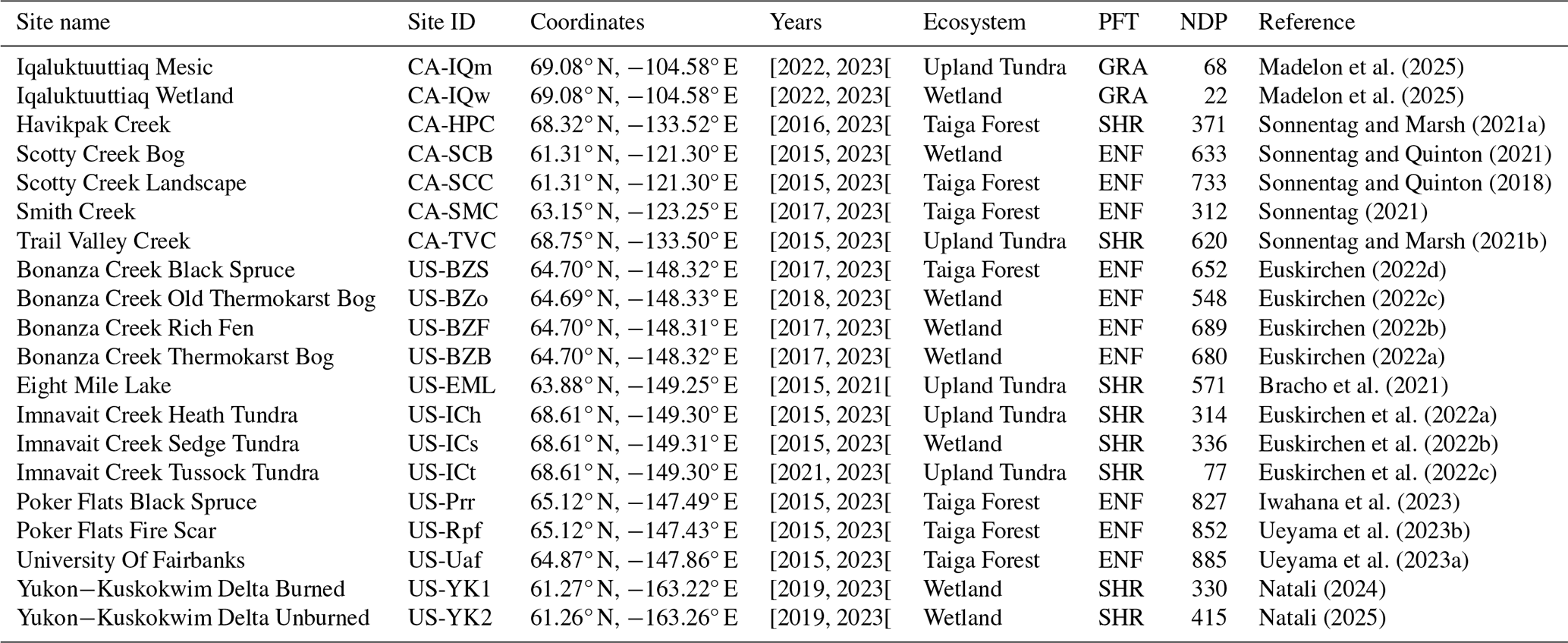
NEE, GPP, and ER data were collected from 20 EC towers located in AS environments (Fig. 1), all within the NASA Arctic-Boreal Vulnerability Experiment (ABoVE) study domain (https://above.nasa.gov/sites.html, last access: 15 January 2026). The dataset spans from April 2015 through December 2022 (Table 1) and includes
-
half-hourly fluxes from 13 EC towers in Alaska, downloaded from the AmeriFlux Network website (https://ameriflux.lbl.gov, last access: 21 August 2025).
-
half-hourly fluxes from 7 EC towers in western Canada, provided directly by the principal investigators to ensure the use of the most up-to-date records; some of these sites are not yet available on the AmeriFlux Network website.
EC towers measure NEE by quantifying the turbulent vertical exchange of CO2 in the surface layer of the atmospheric boundary layer (typically within the lowest tens of meters), where turbulence dominates the airflow (Aubinet et al., 2012; Burba, 2013, 2022). The spatial footprint can extend up to 1 km or more, but remains complex to estimate and varies with wind direction, wind speed, and tower height (Leclerc and Thurtell, 1990; Schuepp et al., 1990; Aubinet et al., 2012; Webb et al., 2016). GPP and ER are derived from NEE using flux-partitioning methods selected by the investigators at each EC tower. In this study, we placed confidence in these flux-partitioning methods and considered the resulting partitioned GPP and ER values to be credible representations of the underlying processes and suitable for use as reference data for model calibration and evaluation. Additional information on NEE, and the derived GPP and ER is provided in Appendix A. EC NEE, GPP, and ER were averaged from 30 min intervals to daily time steps, using at least 24 out of the theoretical 48 data points available per day. Hereafter, NEEEC, GPPEC, and EREC refer to the daily means of EC NEE, GPP, and ER.

Figure 1Locations of the 20 eddy covariance (EC) towers providing measurements of net ecosystem CO2 exchange (NEEEC), NEE-derived gross primary production (GPPEC) and ecosystem respiration (EREC) from April 2015 to December 2022. The High Arctic, Low Arctic and Subarctic zones were delineated following the Conservation of Arctic Flora and Fauna (CAFF) working group of the Arctic Council, using Moderate Resolution Imaging Spectroradiometer (MODIS) and Landsat imagery (Potapov et al., 2008). The permafrost extent is estimated in percent areal coverage (Brown et al., 2002): continuous (>90 %–100 % areal extent), discontinuous (>50 %–90 %), sporadic (10 %–50 %) and isolated patches (<10 %). Due to overlapping, a single color dot may represent up to four EC towers on the map. Information for each EC tower is listed in Table 1. The figure was inspired by Madelon et al. (2025) and Mavrovic et al. (2023a).
Table 1List of the 20 eddy covariance (EC) tower sites used in this study. Ecosystem types were assigned based on site descriptions while plant functional type (PFT) classes were assigned using the Moderate Resolution Imaging Spectroradiometer (MODIS) MCD12Q1 type 5 product (Friedl and Sulla-Menashe, 2019). GRA, SHR, and ENF stand for grassland, shrubland, and evergreen needleleaf forest, respectively. Column 7 shows the number of data points (NDP) within the EC net ecosystem CO2 exchange (NEEEC), gross primary production (GPPEC), and ecosystem respiration (EREC) time series after daily averaging and data filtering (see Sects. 2 and 4.2).
All EC towers considered in this study are located in the tundra and taiga biomes, in areas underlain by sporadic, discontinuous, or continuous permafrost (Fig. 1). Permafrost (ground that has remained frozen for more than 2 years) lies beneath an active layer that thaws during the growing season, enabling plant growth, as roots can only establish in thawed soil (Blume-Werry et al., 2019). Permafrost also restricts surface drainage, promoting water saturation and slowing decomposition rates (Wania et al., 2009; Robinson and Moore, 2000; Rouse et al., 1997; Maltby and Immirzi, 1993). These conditions can favor the formation of wetlands, including peatlands as well as other seasonally or permanently waterlogged ecosystems, across both tundra and taiga biomes (Treat et al., 2022). Based on site descriptions, EC towers were grouped into three distinct ecosystem types (Table 1):
-
Taiga forests: 7 EC towers are located in taiga forests, characterized by a vertically stratified vegetation structure, with an open canopy of coniferous trees and an understory of shrubs, mosses, and lichens (Crawford, 2013; Juday, 2025).
-
Upland tundra: 5 EC towers are located in upland tundra, which may exhibit lower vegetation density and diversity, as well as reduced soil biological activity, compared with taiga forests (Crawford, 2013; Hagedorn et al., 2025). The landscape is treeless and dominated by dwarf shrubs, grasses, sedges, mosses, and lichens, as plant growth is constrained by cold temperatures, short growing seasons, and the shallow depth of the permafrost active layer (Crawford, 2013; Hu and Bliss, 2025; Juday, 2025; Péwé, 2025).
-
Wetlands: 8 EC towers are located in wetlands, where the term “wetland” refers to a wide range of types, including peatlands, bogs, fens, marshes, wet meadows, and shrub swamps, present in both tundra and taiga biomes. Compared with taiga forests and upland tundra, wetlands may exhibit higher species richness (McPartland et al., 2019) and localized microtopography, such as hummocks and hollows, whose characteristics depend on water table depth (Rouse et al., 1997; Zhang et al., 2024).
The L4C model provides global, daily estimates of NEE, GPP, and ER at 9 km resolution from 31 March 2015, to the present (Jones et al., 2017; Kimball et al., 2025). It takes as inputs
-
A static global plant functional type (PFT) classification at 500 m resolution, retrieved from the Moderate Resolution Imaging Spectroradiometer (MODIS) MCD12Q1 Type 5 product (Friedl and Sulla-Menashe, 2019).
-
Eight-day fraction of photosynthetically active radiation (canopy-intercepted FPAR) and leaf area index (LAI) data at 500 m resolution, retrieved from the Visible Infrared Imaging Radiometer Suite (VIIRS) VNP15A2H product (Myneni and Knyazikhin, 2018).
-
Daily means of three-hourly data at 9 km resolution, retrieved from the SMAP SPL4SMGP product version 8 (Reichle et al., 2025a), including 10 cm deep soil temperature (ST10), surface skin temperature, incident shortwave solar radiation (SWin), surface soil moisture (SSM), and rootzone soil moisture (RZSM). SSM and RZSM estimates are obtained by assimilating SMAP L-band brightness temperature observations into the Goddard Earth Observing System Version 5 Catchment Land Surface Model (GEOS-5 CLSM) (Reichle et al., 2019).
-
Daily vapor pressure deficit (VPD) and minimum air temperature (MNT) at 0.25° (approximately 25 km resolution), retrieved from the GEOS-5 Forward Processing (FP) product (Lucchesi, 2018).
SWin is combined with FPAR to compute canopy-absorbed photosynthetically active radiation (APAR), assuming that PAR constitutes 45 % of SWin, as follows:
RZSM is rescaled using a normalized logarithmic transformation (Jones et al., 2017), and SSM is converted from volumetric units to relative wetness units. With the exception of APAR, the variables MNT, VPD, RZSM, ST, and SSM affect GPP and ER estimation only after being converted into stress scalars, denoted as SMNT, SVPD, SRZSM, SST, and SSSM. The derivation of these stress scalars is described later in Eq. (7a–e).
The L4C model runs at a daily time step and is defined as follows:
GPP is modeled using a light-use efficiency approach (Jones et al., 2017; Xiao et al., 2013), where ϵmax represents the bulk environmental reduction in PAR conversion efficiency. AR is modeled as a fixed proportion of GPP, determined by the coefficient α. HR is estimated using a cascading three-pool SOC decomposition model (Ise and Moorcroft, 2006; Kimball et al., 2008; Jones et al., 2017), assuming that carbon fixed from atmospheric CO2 through GPP enters the SOC pools as litterfall (Lfall). The daily SOC change for each of the three SOC pools is specified as:
SOC1, SOC2, and SOC3 represent the labile, structural, and recalcitrant SOC pools, respectively, with corresponding decay rates k1, , and . The model parameters λ and η account for the fraction of Lfall allocated to the SOC1 and SOC2 pools, and the fraction of material transferred from the SOC2 pool to the SOC3 pool, respectively. The parameters ϵmax, kl, λ, and η are treated as free parameters estimated during the optimization process. The model integration step dt is set to one day.
In the L4C model version 7, Lfall was derived as a constant daily fraction of the mean annual estimated net primary productivity (NPP), as follows:
and denote the mean annual NPP and GPP, respectively, and the daily fraction is set to for leap years. Instantaneous NPP is initially derived as . In the L4C model version 8, the allocation timing was changed from constant to dynamic, and is now determined using a leaf-loss function (Lloss), derived from climatological LAI, as follows:
Here, fE represents the proportion of the canopy that is evergreen. Lloss is computed using a triangular moving average centered on the current time step, where weights increase linearly toward the center. It represents the difference between lagged and leading climatological LAI values (Endsley et al., 2022).
In Eqs. (3a–b) and (4a–c), the stress scalars SMNT, SVPD, SRZSM, SST, and SSSM represent the ecosystem responses to their respective environmental variables and are defined as follows:
Each stress scalar ranges from 0 to 1, where a value of 0 indicates that the environmental variable fully constrains model estimates, while a value of 1 indicates no constraint. The thresholds MNTmin, MNTmax, VPDmin, VPDmax, RZSMmin, RZSMmax, SSMmin, and SSMmax are free parameters estimated during the optimization process. These are used as model thresholds and do not correspond to the actual minimum or maximum values within the time series. Similarly, β0 is a free parameter, while β1 and β2 are fixed at 66.02 and 227.13 K, respectively (Kimball et al., 2025). The behavior of the ecosystem response functions is shown in Appendix B, Fig. B1(A1–C1). The GPP formulation originally includes a stress scalar based on the freeze–thaw state, computed using surface skin temperature from the SMAP SPL4SMGP product (Jones et al., 2017; Kimball et al., 2025). However, it is not shown here, as this study focuses on the growing season.
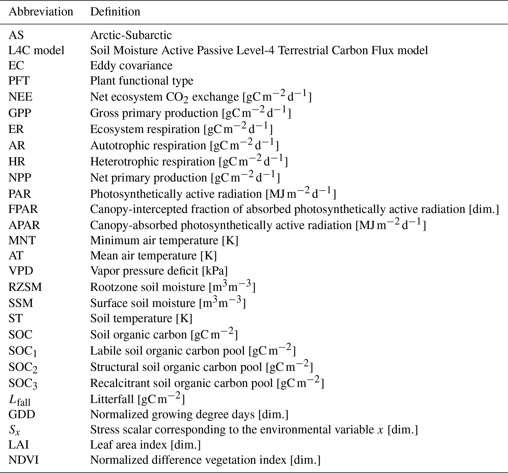
L4C model estimates are initially derived at a 1 km sub-grid resolution for up to 8 MODIS MCD12Q1 PFT classes, and then averaged to 9 km resolution. In this study, only the L4C model estimates corresponding to the PFT class in which the EC towers are located were considered (Table 1). A total of two towers are located in the grassland (GRA) class, 8 in the shrubland (SHR) class, and 10 in the evergreen needleleaf forest (ENF) class. Hereafter, NEEL4C, GPPL4C, and ERL4C refer to daily estimates derived from the L4C model, which were retrieved from the SMAP SPL4CMDL product version 8. Frequently used abbreviations throughout this study are listed in Table 2.
4.1 Arctic-Subarctic adapted model formulations
In this study, we explored alternative GPP and ER model formulations that retain the core GPP and ER equations of the original L4C model version 8. We aimed to preserve the structure and variable set of the original L4C model while enabling the incorporation of constraints or additional flexibility guided by literature-based findings on ecosystem responses and flux-partitioning methods. Five different formulations are presented for both GPP and ER, with each formulation building incrementally on the previous one by incorporating earlier modifications along with additional adjustments. Testing modifications incrementally, rather than independently, allowed us to determine whether their interactions improved or degraded model performance.
The GPP formulations, labeled GPP1 through GPP5, mainly adjust ecosystem responses to environmental variables and are defined as follows (Table 3):
-
GPP1: Under sub-freezing air temperatures, photosynthetic activity is expected to be severely reduced, approaching cessation (Schaefer et al., 2012; Ensminger et al., 2004; Bowling et al., 2018; Parazoo et al., 2018). This behavior is not well represented in the original L4C model, where SMNT still remains near 0.5 at 270 K (Figs. 2, 3, 4(A2)), indicating that GPP capacity is reduced by only half at this temperature. In the proposed formulation, GPP is ensured to cease when MNT is equal to or below 273.15 K by fixing the minimum threshold (MNTmin) of SMNT to 273.15 K (Eq. 7a).
-
GPP2 (defined as GPP1 with additional adjustments): Some flux-partitioning methods use a nonlinear light-response curve to partition NEEEC into GPPEC and EREC (Lasslop et al., 2010b; Runkle et al., 2013), capturing the saturation of leaf-level photosynthesis at high solar irradiance. In the original L4C model, APAR directly scales the dynamic range of GPP and is not transformed through a transfer function into a stress scalar, as is the case for the other environmental variables (Eq. 3a). In GPP2, this linear dependence is replaced by a nonlinear stress scalar, SAPAR, inspired by the light-response curve, which is defined as follows:
At low APAR, GPP increases rapidly, but as APAR increases, the rate of increase slows down, and GPP asymptotically approaches a maximum value, GPPmax. This behavior is shown in Appendix B, Fig. B1(D1). GPPmax and APARcrit are free parameters estimated during the optimization process.
-
GPP3 (defined as GPP2 with additional adjustments): In the original L4C model, GPP responds linearly to MNT, VPD, and RZSM (Eq. 7a, b, c). In GPP3, GPP responses to these variables are modeled with increased flexibility, with no assumed shape other than monotonicity, to allow varying rates of change across different ranges. To achieve this, they are redefined as logistic ramp functions:
In this formulation, the thresholds MNTmin, MNTmax, VPDmin, VPDmax, RZSMmin, and RZSMmax are used to scale the stress scalars between 0 and 1, and are fixed to 273.15, 293.15 K, 0, 2.5 kPa, 0, and 1 m3 m−3, respectively. The parameters MNTcrit, γMNT, VPDcrit, γVPD, RZSMcrit, and γRZSM are treated as free parameters and are estimated during the optimization process. The behavior of the logistic ramp functions is illustrated in Appendix B, Fig. B1(A2, B2).
-
GPP4 (defined as GPP3 with additional adjustments): Growing degree days (GDD) are widely used in agricultural and ecological studies as a proxy to plant development (Fotouo Makouate and Zude-Sasse, 2025), and have recently been used to develop a phenology scheme that improved GPP modeling in a temperate bog (He et al., 2025). In the present formulation, GDD is incorporated into GPP modeling to capture the vegetation green-up and senescence phases through an additional stress scalar (SGDD). GDD is first derived from mean air temperature (AT) using a base temperature of 273.15 K. It is then normalized for each site and each year using the annual minimum and maximum values, resulting in a normalized range from 0 to 1. This normalization ensures that GDD acts as a seasonal shape or trend driver, rather than a magnitude driver, which is instead represented by the instantaneous variables (APAR, MNT, VPD, and RZSM). Hereafter, GDD refers to normalized GDD and is used to derive SGDD, as follows:
SGDD is defined as a beta-like, bell-shaped function, normalized between 0 and 1 (Appendix B, Fig. B1(C2)). The parameters a and b are treated as free parameters and are estimated during the optimization process.
-
GPP5 (defined as GPP4 with additional adjustments): Some studies have reported that water-saturated soil conditions limit oxygen and nutrient availability to plant roots, restrict cellular respiration, and consequently hinder photosynthetic activity (Kreuzwieser et al., 2004; Nawaz et al., 2025). Additionally, Peng et al. (2024) showed that the relationship between GPP and soil moisture may follow a bell-shaped curve at EC tower sites with PFTs similar to those in the present study (e.g., ENF, SHR, GRA; Table 1). A similar response has also been reported for peatlands (Valkenborg et al., 2023). In GPP5, it is similarly assumed that GPP peaks at an optimal RZSM level, beyond which excessive moisture reduces efficiency. This assumption is tested by redefining SRZSM as a beta-like, bell-shaped function, analogous to SGDD (Eq. 10b and Fig. B1(C2) in Appendix B):
The parameters a and b are treated as free parameters and are estimated during the optimization process.
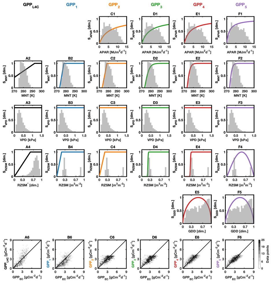
Figure 2Ecosystem responses used to compute modeled gross primary production (GPP) from the L4C model (GPPL4C, column A) and from the Arctic-Subarctic (AS) adapted formulations (GPP1 through GPP5, columns B–F) in upland tundra during the growing season. The ecosystem responses are expressed as stress scalars, Sx, for each environmental variable x, where x represents absorbed photosynthetically active radiation (APAR), minimum air temperature (MNT), vapor pressure deficit (VPD), root zone soil moisture (RZSM), and normalized growing degree days (GDD). In the background of each subplot, the histogram of the corresponding environmental variable is shown in light grey. All ecosystem responses of a given model formulation are calibrated jointly using eddy covariance GPP (GPPEC) as reference, and not based on the histogram values. In subplot A4, RZSM* refers to the normalized RZSM used as input in the original L4C model. Subplots A1 and B1 are omitted because APAR is used as a direct input, rather than through a stress scalar, in GPPL4C and GPP1 formulations. Similarly, subplots A5-D5 are omitted because GDD is not used as input in the GPPL4C, GPP1, GPP2, and GPP3 formulations. Refer to Sects. 3 and 4.1 for a detailed description of each model formulation. The last row displays scatter plots between modeled GPP against GPPEC. It is a spatiotemporal comparison, accounting for both temporal and spatial variability. It includes all available GPPEC data points for upland tundra after filtering, including those used for calibration (1650 data points; Sect. 4.3).
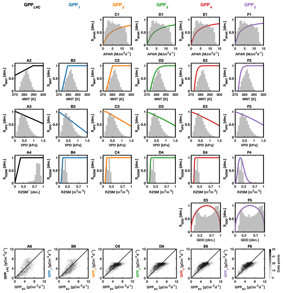

Table 3Summary of the specificity of each Arctic-Subarctic (AS) adapted model formulation of the L4C model. Column 1 lists the gross primary production (GPP) and ecosystem respiration (ER) formulations, labeled GPP1 through GPP5 and ER1 through ER5, respectively. The free parameters estimated during the optimization process are provided in column 2. Each GPP and ER formulation is incrementally built on the previous one by incorporating its modifications along with an additional change summarized in column 3. APAR, MNT, VPD, RZSM, SSM, GDD, NPP, Lfall, SOC, Rbase, denote absorbed photosynthetically active radiation, minimum air temperature, vapor pressure deficit, rootzone soil moisture, surface soil moisture, normalized growing degree days, net primary productivity, litterfall, soil organic carbon, and baseline heterotrophic respiration, respectively. Refer to Sects. 3 and 4.1 for a description of each model formulation and parameter.
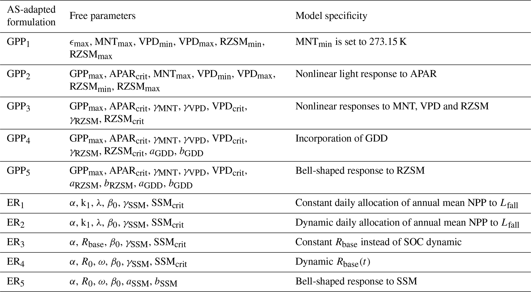
Regarding the ER modeling, we tested different formulations for the HR component while leaving the AR component unchanged. The ER formulations, labeled ER1 through ER5, are described below (Table 3):
-
ER1: Rather than using the the Lfall estimation scheme from the baseline L4C model version 8, ER1 instead adopts the one from version 7 (Eq. 5). The L4C model transitioned from version 7 to version 8 over the course of the present study was conducted, during which the Lfall estimation scheme was modified. The version 7 scheme was retained to enable comparison with the one introduced in version 8. Additionally, HR response to SSM (SSSM) is redefined as a logistic ramp, analogous to SRZSM in GPP3 (Eq. 9c and Fig. B1(A2)). The original linear response (Eq. 7d) was directly replaced because the logistic ramp can reproduce a linear behavior if the relationship between SSM and HR is actually linear. The ER response function to ST is unchanged but was recalibrated (Eq. 7e).
-
ER2 (defined as ER1 with additional adjustments): The Lfall estimation scheme is reverted to that of the baseline L4C model version 8. Hence, ER1 and ER2 differ only in the Lfall estimation scheme (version 7 vs. 8), isolating its impact.
-
ER3 (defined as ER2 with additional adjustments): None of the established flux-partitioning methods requires SOC data to derive GPP and ER from NEE (Reichstein et al., 2005; Lasslop et al., 2010b; Runkle et al., 2013; Helbig et al., 2017a). Consequently, in ER3, we aimed to capture the added value of incorporating SOC dynamics in ER modeling. To this end, SOC dynamics are replaced by a single constant representing a baseline heterotrophic respiration rate, (Rbase), as follows:
The parameter Rbase is treated as a free parameter and is estimated during the optimization process.
-
ER4 (defined as ER3 with additional adjustments): In the present formulation, we aimed to mimic the flux-partitioning methods that derive Rbase every few days (Reichstein et al., 2005; Lasslop et al., 2010b; Runkle et al., 2013; Helbig et al., 2017a). Rbase is then redefined as:
This follows a first-order auto-regressive (AR1) approach, in which the current value depends on the previous one and the 7 d backward mean of the product of temperature and moisture stress scalars (), weighted by the parameter ω (ranging from 0 to 1). This approach introduces acclimation behavior by smoothing short-term variability in environmental conditions. The parameters R0 and ω are treated as free parameters and are estimated during the optimization process.
-
ER5 (defined as ER4 with additional adjustments): Endsley et al. (2022) showed that including an O2 diffusion limitation in the HR response to SSM, which penalizes HR rates under high SSM conditions, improved seasonal ER performance. In ER5, we adopted the beta-like, bell-shaped function, analogous to SRZSM in GPP5 (Eq. 11), to model HR response to SSM. This avoids to collect or estimate O2 concentration data while still representing diminishing returns on HR under high SSM conditions.
In this study, daily VPD and MNT were retrieved from the Modern-Era Retrospective Analysis for Research and Applications, Version 2 (MERRA-2), M2T1NXSLV Version 5.12.4 product (Gelaro et al., 2017), instead of the GEOS-5 FP product, because it is sparsely documented. MERRA-2 re-analysis dataset is better constrained by observations, exhibits a climatology comparable to GEOS-5 FP and is used in the L4C model calibration due to its longer period of record. AT, required to derive GDD, was also retrieved from the MERRA-2 M2T1NXSLV product. Finally, RZSM and SSM from the SMAP SPL4SMGP product were retained in volumetric units (m3 m−3), unlike in the original L4C model.
4.2 Growing season timing and data filtering
GPPEC was used as an indicator to identify the growing season (Gonsamo et al., 2013). For each EC tower, GPPEC values below the noise threshold of 0.05 were first attributed to the winter season and removed. Among the remaining values, those below the 10th percentile were considered part of the shoulder seasons (i.e., transitional periods between fully frozen and fully thawed states) and were excluded. The growing season is more commonly defined using fixed fractions of annual maximum GPPEC rather than percentile-based thresholds (Panwar et al., 2023; Luo et al., 2025). However, such approaches rely on the assumption that the annual maximum GPPEC is robustly captured each year, which may not hold due to data gaps for instance. In addition, a previous study has shown that the growing season identification is sensitive to the chosen fraction of annual maximum GPPEC, indicating a lack of consensus on an optimal threshold (Panwar et al., 2023). In contrast, the percentile-based approach used here provides a distribution-based criteria that is less sensitive to extreme values and inter-annual variability, ensuring consistency across years. For instance, two years with the same growing season timing (i.e., identical start and end dates) but different photosynthetic peaks are treated identically, which would not be the case when using the annual maximum GPPEC. Although the 10th percentile threshold may not be optimal for each GPPEC time series, it is consistent with the structure of the mean seasonal cycle of GPPEC, where it separates winter and shoulder seasons from the growing season (Fig. B2). In addition, similar separations are obtained when using thresholds within the 5th–15th percentile range, indicating low sensitivity to the chosen percentile. Finally, GPPEC and EREC values above the 99th percentile were treated as outliers and removed.
Complementary filtering flags were applied to ensure biophysical plausibility of root-level soil activity and photosynthesis during the growing season from a modeling perspective. The specific criteria for these flags are as follows:
-
ST10 cm ≥ 275.15 K (i.e., 2 °C above freezing)
-
ST20 cm ≥ 275.15 K
-
ST39 cm ≥ 275.15 K (applied to ENF sites only, see Table 1)
-
MNT ≥ 275.15 K
ST20 cm and ST39 cm refer to soil temperature at 20 and 39 cm depths, respectively, and were retrieved from the SMAP SPL4SMGP product. For the remainder of this study, ST refers to ST10 cm as ST20 cm and ST39 cm are not used further.
After filtering, a total of 1650 data points (23 %) remained for the upland tundra ecosystem, 4632 data points (33 %) for the taiga forest ecosystem, and 3653 data points (30 %) for the wetland ecosystem (Table 1).
4.3 Model formulation calibration
The AS-adapted GPP and ER formulations were calibrated separately for each ecosystem type (upland tundra, taiga forests, and wetlands), using GPPEC and EREC as reference targets. The optimization framework for calibration used least-squares minimization via the MATLAB lsqcurvefit function (MathWorks, Inc., 2023), which minimizes the sum of squared differences between the model outputs and target values. This is an unconstrained optimization, with no additional penalty terms applied. To mitigate overfitting, the optimization process was repeated 100 times using different random training (70 %) and testing (30 %) subsets of the data for each ecosystem type: 1155 (495) data points for upland tundra, 3243 (1389) for taiga forests and 2557 (1096) for wetlands. In each optimization run, model parameters were estimated using the corresponding training subset, and final parameter values were defined as the median of the parameter estimates across all 100 runs. This approach aimed to capture diverse data combinations and promote a more stable and representative parameterization by smoothing out the influence of outliers or any individual biased subset. A 70 % subset size was arbitrarily chosen to balance between providing sufficient data for robust model calibration and retaining enough data variability across the 100 iterations (Martinez Molera, 2025). Contrary to the global calibration of the original L4C model, no reference SOC data were used to constrain the recalibration over the AS environments. As a result, in ER1 and ER2, only the SOC1 pool was modeled to avoid potential parameter compensation and to prevent unrealistic SOC distribution across the original three pools. This reduction in the number of SOC pools constitutes an additional adjustment for ER1 and ER2 that is confounded with the change in Lfall estimation scheme (Sect. 4.1). An initial guess was necessary for SOC1 on 31 March 2015, to explicitly solve the SOC dynamics, since the system is formulated recursively and requires a starting value to iterate forward in time (Eq. 4). 31 March 2015, was chosen as the start of the simulation because it precedes the first date of the period of study. The initial guess was set to 0 gC m−2 for the first spin-up iteration, providing a neutral starting point to avoid biasing the early simulation. It was subsequently updated using the SOC value on 31 March 2022, corresponding to the last 31 March within the study period. A total of 20 spin-up iterations were performed.
4.4 Model formulation evaluation
For each ecosystem type, the AS-adapted GPP and ER formulations were evaluated spatiotemporally, capturing the combined effects of spatial and temporal variability, with GPPEC and EREC used as reference targets. For each of the 100 optimization runs (Sect. 4.3), the Pearson correlation coefficient (r), the unbiased root mean square error (ubRMSE), and the bias (B) were computed separately for the training and testing subsets, enabling the assessment of model calibration and generalization, respectively. Median values across the 100 runs were reported. The trade-off between goodness of fit and model complexity was quantified using the Akaike Information Criteria (AIC) and Bayesian Information Criteria (BIC), which were applied on the training subsets. The best-performing ER and GPP formulations were identified based on the lowest ΔAIC and ΔBIC values, defined as AIC − AICL4C and BIC − BICL4C, respectively. Median values across the 100 runs were reported. As a complementary analysis, site-level (temporal-only) performance was evaluated for each EC tower by computing r, ubRMSE, and B using model outputs obtained with the median parameter values across the 100 runs. For this analysis, training and testing data were pooled, and median metrics across EC towers were reported.
As the ER formulations require GPP as an input, all 25 possible ER configurations were systematically evaluated (ER1 through ER5 combined with GPP1 through GPP5). This approach also yields 25 corresponding NEE configurations, as NEE is defined as the difference between ER and GPP (Eq. 3). Evaluating all combinations enables assessment of whether the best-performing GPP formulation is associated with the best-performing ER formulation, and whether the combination of the best-performing ER and GPP formulations also results in the most accurate NEE configuration. It additionally enables identification of cases where GPP and ER formulations that perform less well individually (relative to EREC and GPPEC) nevertheless yield a more accurate NEE configuration (relative to NEEEC). Such behavior may arise because errors in modeled ER and GPP can either compensate or accumulate when computing NEE.
The 25 NEE configurations were evaluated following the same approach as for the GPP and ER formulations, using NEEEC as the reference target. Although NEE configurations were not directly calibrated, the same training and testing subsets were retained for consistency with the GPP and ER formulation evaluations, ensuring that each NEEEC value was paired with its corresponding GPPEC and EREC values.
Because the evaluation of 25 ER formulations produces many metrics, only ER1 through ER5 using the GPP input that yields the best performance are presented in the main text. Results for all configurations are provided in Appendix D. This avoids bias arising from the choice of GPP input when comparing ER formulations. For NEE, summarized performance for all configurations is presented in the main text, while detailed results are provided in Appendix E. Hereafter, NEEi, j denotes modeled NEE computed as ERi − GPPj.
5.1 Gross primary production
5.1.1 Upland tundra
Based on the spatiotemporal evaluation of the testing splits for upland tundra (Table 4), GPP1 performs better than GPPL4C in terms of B and ubRMSE (−0.33 vs. 0.41 and 1.19 vs. 1.46 , respectively). However, GPPL4C achieves a higher r value (0.56 vs. 0.64). Introducing a nonlinear light-response in GPP2 (Eq. 8) leads to better performance compared with GPP1, reducing B from −0.33 to −0.02 . In addition, ubRMSE decreases, and r increases, approaching the r observed for GPPL4C. Replacing linear ramps with logistic ramps to simulate ecosystem responses in GPP3 (Eq. 9) increases model complexity but provides limited improvement over GPP2. GPP4 incorporates GDD through an additional stress scalar (Eq. 10). This results in improved r and ubRMSE compared with GPP3 (0.75 vs. 0.64, and 0.84 vs. 0.96 , respectively). In GPP5, a bell-shaped function is used to simulate the influence of RZSM (Eq. 11). This further improves r and ubRMSE, though B slightly increases (−0.03 vs. −0.01 ).
Table 4Performance of modeled gross primary production (GPP) against daily averaged eddy covariance (EC) GPP (GPPEC) for upland tundra, taiga forests, and wetlands during the growing season. GPPL4C refers to outputs from the original L4C model, while GPP1 through GPP5 correspond to the five Arctic–Subarctic (AS) adapted formulations (Sects. 3 and 4.1). The Pearson correlation coefficient is denoted by r (dimensionless), and ubRMSE and B denote the unbiased root mean square error and bias, respectively (in ). A positive (negative) B indicates overestimation (underestimation) of GPPEC. (a) Spatiotemporal performance metrics derived from 100 random splits (70 % training, 30 % testing), accounting for both spatial and temporal variability. The total number of data points used for training (testing) is 1155 (495) for upland tundra, 3243 (1389) for taiga forests, and 2557 (1096) for wetlands (Sect. 4.3). Median values across the 100 splits are reported. (b) Site-level (temporal-only) performance metrics computed for each EC tower using model outputs obtained with the median parameter values across the 100 splits. Metric values are reported as the median across towers. For this analysis, training and testing data are pooled.
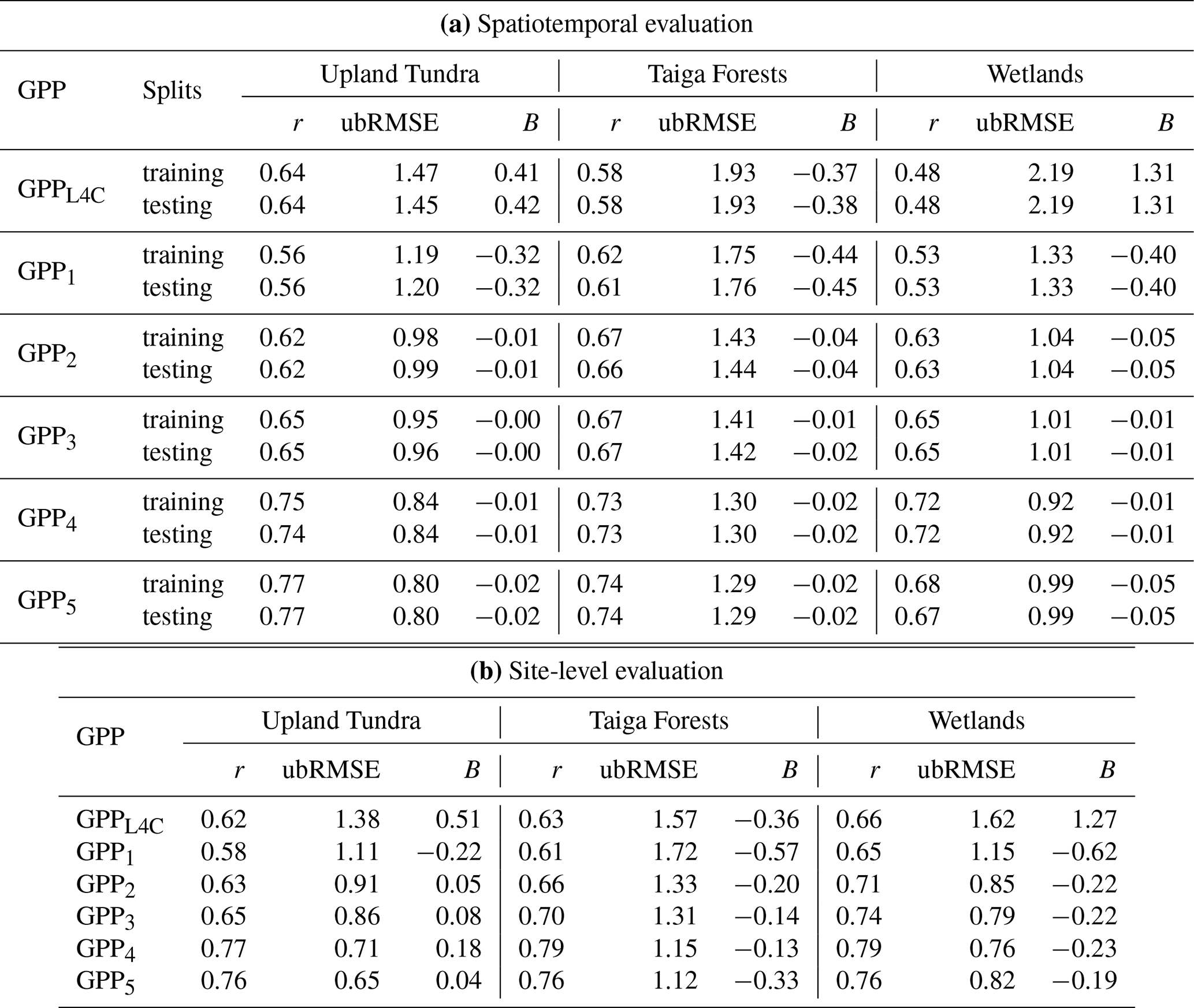
Considering the site-level evaluation (Table 4), GPP4 and GPP5 exhibit the highest r (0.77 vs. 0.76) and the lowest ubRMSE (0.65 vs. 0.71 ). In contrast, GPP5, GPP3, and GPP2 show the lowest B with 0.04, 0.05, and 0.08 , respectively.
Across all formulations, SVPD remains equal to 1 throughout the entire range of VPD variability (Fig. 2(B3–F3)). The use of a non linear light-response in GPP2 introduces an early saturation (Fig. 2(B6–F6)), where modeled GPP peaks are lower than those of GPPEC. This premature flattening is progressively reduced in GPP4 and GPP5, due to the incorporation of GDD and the use of a bell-shaped function for simulating RZSM influence.
The lowest ΔAIC and ΔBIC are obtained for GPP5, followed by GPP4, GPP3, GPP2 and GPP1 in last place (Table C1). For GPP2 and GPP3, ΔAIC and ΔBIC are equal within each subset (training or testing) because both formulations have the same number of free parameters as GPPL4C.
5.1.2 Taiga forests
The spatiotemporal evaluation of the testing splits for taiga forests (Table 4) indicates that GPP1 performs better than GPPL4C in terms of r (0.62 vs. 0.58) and ubRMSE (1.75 vs. 1.93 ), although GPP1 shows higher B (−0.44 vs. −0.37 ). As in upland tundra (Sect. 5.1.1), introducing a nonlinear light-response in GPP2 (Eq. 9) leads to overall better performance compared with GPP1, notably reducing B from −0.44 to −0.05 . GPP3 does not offer improvement over GPP2, aside from a slight reduction in B (−0.02 vs. −0.05 ). Due to the inclusion of GDD through an additional stress scalar (Eq. 10), GPP4 outperforms GPP3 (0.73 vs. 0.67 for r, and 1.30 vs. 1.41 for ubRMSE). Switching to a bell-shaped function for simulating RZSM influence in GPP5 (Eq. 11) does not result in improved performance compared with GPP4.
Considering the site-level evaluation (Table 4), the highest r are obtained for GPP4 and GPP5 (0.79 vs. 0.76). These two formulations also achieve the lowest ubRMSE, with 1.12 for GPP5 and 1.15 for GPP4. GPP4 and GPP4 exhibits the lowest B (−0.13 vs. −0.14 ).
RZSM appears to be a negligible input in GPPL4C, as SRZSM remains equal to 1 throughout the entire range of RZSM variability (Fig. 3(A4)). However, RZSM gains more effect in GPP1 through GPP5, although its effect remains weaker than that of MNT, VPD, and GDD (Fig. 3(B4–F4)). As in upland tundra (Sect. 5.1.1), the use of a nonlinear light-response in GPP2 introduces an early saturation, underestimating GPPEC peaks (Fig. 3(B6–F6)). However, this premature flattening persists in GPP4 and GPP5, despite the incorporation of GDD and the use of a bell-shaped function for simulating RZSM influence.
The lowest ΔAIC and ΔBIC are obtained for GPP5, closely followed by GPP4, then GPP3, GPP2 and GPP1 in last place (Table C1). For GPP2 and GPP3, ΔAIC and ΔBIC are equal within each subset (training or testing) because both formulations have the same number of free parameters as GPPL4C.
5.1.3 Wetlands
Based on the spatiotemporal evaluation of the testing splits for wetlands (Table 4), GPP1 outperforms GPPL4C, notably exhibiting reduced ubRMSE and B (1.33 vs. 2.18 , and −0.39 vs. 1.32 , respectively). As seen in upland tundra and taiga forests (Sects. 5.1.1 and 5.1.2), introducing a nonlinear light-response in GPP2 (Eq. 8) results in improved r (0.63 vs. 0.53), reduced ubRMSE (1.04 vs. 1.33 ), and reduced B (−0.05 vs. −0.39 ), compared with GPP1. GPP3 shows only a minor improvement over GPP3. Due to the inclusion of GDD through an additional stress scalar (Eq. 10), GPP4 outperforms GPP3 (0.72 vs. 0.65 for r, and 0.92 vs. 1.01 for ubRMSE). In contrast to upland tundra and taiga forests (Sect. 5.1.1 and 5.1.2), using a bell-shaped function for simulating RZSM influence in GPP5 (Eq. 11), result in degraded performance compared with GPP4.
Considering the site-level evaluation (Table 4), GPP4 and GPP5 exhibit the highest r (0.79 vs. 0.76). GPP4 and GPP3 exhibits the lowest ubRMSE (0.76 vs. 0.79 , respectively), closely followed by GPP5 (0.82 ) and GPP3 (0.85 ). B is similar for GPP2 through GPP5, with −0.22, −0.22, −0.23, and −0.19 , respectively.
Similar to upland tundra (Sect. 5.1.1), SVPD remains equal to 1 throughout the entire range of VPD variability across all formulations (Fig. 4(B3–F3)). Likewise, as observed in taiga forests (Sect. 5.1.2), RZSM appears to be a negligible input in GPPL4C, with SRZSM staying equal to 1 throughout the entire range of RZSM variability (Fig. 4(A4)). However, RZSM gains a considerable effect in GPP1 through GPP5, especially under dry conditions (Fig. 4(B4–F4)). The introduction of the nonlinear light-response in GPP2 triggers an early saturation (Fig. 4(B6–F6)), that persists throughout GPP5.
In contrast to upland tundra and taiga forests (Sects. 5.1.1 and 5.1.2), the lowest ΔAIC and ΔBIC are obtained for GPP4, followed by GPP5, GPP3, GPP2, and GPP1 in last place (Table C1). For GPP2 and GPP3, ΔAIC and ΔBIC are equal within each subset (training or testing) because both formulations have the same number of free parameters as GPPL4C.
5.2 Ecosystem respiration
For upland tundra and taiga forests, ER formulations using GPP5 as input are compared, as GPP5 yielded the lowest ΔAIC and ΔBIC (Sect. 5.1.1, 5.1.2). For wetlands, the set using GPP4 as input is compared instead, because GPP4 achieved the lowest ΔAIC and ΔBIC for this ecosystem type (Sect. 5.1.3). Results for all 25 ER formulations are provided in Tables D1–D6.
5.2.1 Upland tundra
Based on the spatiotemporal evaluation of the testing splits for upland tundra (Table 5), ER1, which uses the approach where mean annual NPP is allocated uniformly across the year to Lfall (Eq. 5), performs better than ERL4C. It exhibits higher r (0.52 vs. 0.44), reduced ubRMSE (0.72 vs. 0.99 ), and reduced B (−0.12 vs. 0.37 ). Switching to the dynamic allocation in ER2 (Eq. 6) leads to enhanced r (0.61) and ubRMSE (0.64 ) compared with ER1. Using a constant Rbase term instead of a SOC model in ER3 (Eq. 12) results in r and ubRMSE close to those of ER2, and lower B (−0.01 vs. −0.12 ). Using a dynamic Rbase in ER4 (Eq. 13) shows better performance than ER3 with greater r (0.72 vs. 0.60) and reduced ubRMSE (0.53 vs. 0.62 ). In ER5, the use of a bell-shaped function to simulate SSM influence does not provide a clear benefit.
Table 5Same as Table 4, but for ecosystem respiration (ER). GPP5 was used as the GPP input for ER1 through ER5 for upland tundra and taiga forests. For wetlands, GPP4 was used instead.
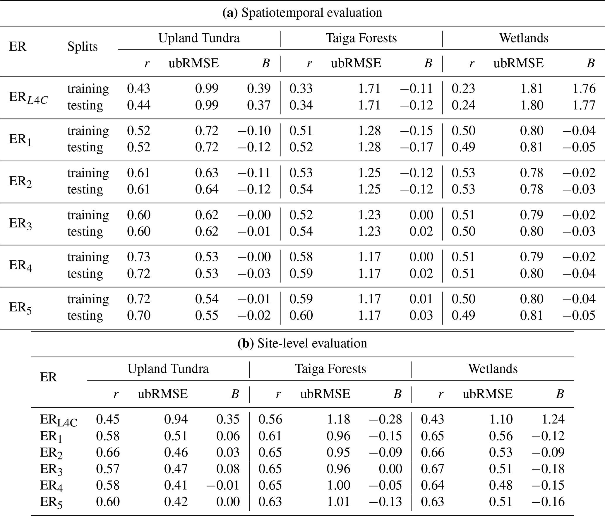
Considering the site-level evaluation (Table 5), the highest r are obtained for ER2 and ER5 (0.66 vs. 0.60). The lowest ubRMSE is observed for ER4 and ER5 (0.41 vs. 0.42 ), closely followed by the other formulations (up to 0.51 for ER1). In terms of B, ER5, ER4, and ER2 show the smallest values with 0.00, −0.01, and 0.03 .
ST appears to have a stronger effect than SSM in ER1 through ER4 (Fig. 5(B1–E1) vs. (B2–E2)). SST mainly oscillates around 0.5, while SSSM rapidly reaches 1 under dry conditions, and wet conditions do not constrain model outputs. In ER5, the use of a bell-shaped function to simulate SSM increases its effect (Fig. 5(F2)), but without any improvement in performance, as previously observed.
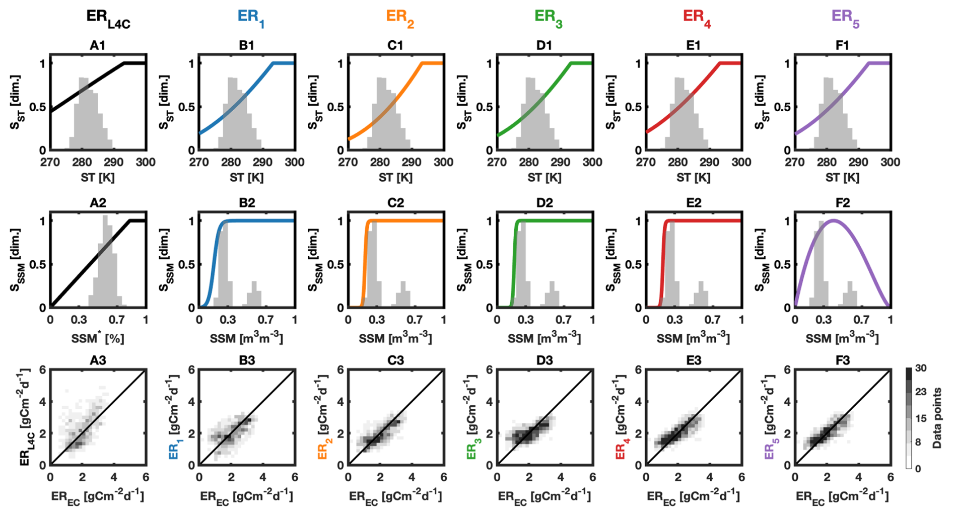
Figure 5Ecosystem responses used to compute modeled ecosystem respiration (ER) from the L4C model (ERL4C, column A) and from the Arctic-Subarctic (AS) adapted formulations (ER1 through ER5, columns B–F) in upland tundra during the growing season. The ecosystem responses are expressed as stress scalars, Sx, for each environmental variable x, where x represents soil temperature (ST) and surface soil moisture (SSM). In the background of each subplot, the histogram of the corresponding environmental variable is shown in light grey. All ecosystem responses of a given model formulation are calibrated jointly using daily-averaged eddy covariance ER (EREC) as reference, and not based on the histogram values. In subplot A2, SSM* refers to the SSM in relative wetness unit used as input in the original L4C model. Refer to Sects. 3 and 4.1 for a detailed description of each model formulation. The last row displays scatter plots between modeled ER against EREC. It is a spatiotemporal comparison, accounting for both temporal and spatial variability. It includes all available EREC data points for upland tundra after filtering, including those used for calibration (1650 data points; Sect. 4.3). GPP5 was used as input for ER1 through ER5 (Sect. 5.2.1).
The lowest ΔAIC and ΔBIC are obtained for ER4, closely followed by ER5, then ER3 and ER2, and ER1 in last place (Table D6). Overall, a similar pattern is observed regardless of the GPP input, and the performance of each ER formulation remains comparable or improves as the GPP input increases in complexity (lowest with GPP1, highest with GPP5; Tables D1–D6).
5.2.2 Taiga forests
Based on the spatiotemporal evaluation of the testing splits for taiga forests (Table 5), ER1 outperforms ERL4C, showing enhanced r (0.52 vs. 0.34), reduced ubRMSE (1.28 vs. 1.71 ), but slightly higher B (−0.17 vs. −0.12 ). Switching from a constant to dynamic allocation of mean annual NPP to Lfall in ER2 (Eq. 6) results in a minor improvement in performance over ER1. Using a constant Rbase term instead of a SOC model in ER3 (Eq. 12) exhibits similar r (0.54 vs. 0.54) and ubRMSE (1.23 vs. 1.25 ), but lower B (0.02 vs. −0.12 ), compared with ER2. Using a dynamic Rbase in ER4 (Eq. 13) shows better performance than ER3 with greater r (0.59 vs. 0.54) and reduced ubRMSE (1.17 vs. 1.23 ). In ER5, the use of a bell-shaped function to simulate SSM influence does not provide a clear benefit.
Considering the site-level evaluation (Table 5), r is similar across formulations, ranging from 0.61 to 0.65. The same pattern is observed for ubRMSE, which ranges from 0.95 to 1.01 . The lowest B are obtained for ER3, ER4, and ER2, with 0.00, −0.05, and −0.09 , respectively.
SSM appears to be a negligible input in ERL4C, as SSSM remains equal to 1 throughout the entire range of SSM variability (Fig. 6(A2)). However, SSM gains more effect in ER1 through ER5, although its effect remains weaker than that of ST (Fig. 6(B2–F2)).

The lowest ΔAIC and ΔBIC are obtained for ER5, nearly tied with ER4, then ER3, ER2, and ER1 in last place. As observed in upland tundra (Sect. 5.2.1), this ranking remains consistent regardless of the GPP input, and the performance of each ER formulation is comparable or improves as the GPP input increases in complexity (lowest with GPP1, highest with GPP5; Tables D1–D6).
5.2.3 Wetlands
Based on the spatiotemporal evaluation of the testing splits for taiga forests (Table 5), ER1 outperforms ERL4C, exhibiting enhanced r (0.49 vs. 0.24), reduced ubRMSE (0.81 vs. 1.80 ), and reduced B (−0.05 vs. 1.77 ). Switching from a constant to dynamic allocation of mean annual NPP to Lfall in ER2 (Eq. 6) slightly increases r (0.53 vs. 0.49), and reduces ubRMSE and B (0.78 vs. 0.81 , −0.03 vs. −0.05 , respectively). Using a constant or dynamic Rbase term instead of a SOC model in ER3 and in ER4 (Eqs. 12 and 13) does not result in enhanced performance. In ER5, the use of a bell-shaped function to simulate SSM influence does not provides any benefits either.
Considering the site-level evaluation (Table 5), r is similar across formulations, ranging from 0.63 to 0.67. The same pattern is observed for ubRMSE, with the highest value assigned to ER1 (0.56 ) and the lowest to ER4 (0.48 ). ER1 and ER2 exhibiting the lowest B, with −0.12 and −0.09 , respectively (Fig. 8(C2)).
As observed in taiga forests (Sect. 5.2.2), SSM appears to be a negligible input in ERL4C, with SSSM staying equal to 1 throughout the entire range of SSM variability (Fig. 7(A2)). However, SSM gains a considerable effect in ER1 through ER5, especially under dry conditions (Fig. 7(B2–F2)). ERL4C may overestimate EREC by up to a factor of two or three (Fig. 7(A3)). This magnitude discrepancy is largely removed in ER1 through ER5, but a pattern persists, in which EREC are systematically overestimated at low values (approximately 0 to 1 ) across all formulations (Fig. 7(B3–F3)).


Figure 8Spatiotemporal performance of modeled net ecosystem CO2 exchange (NEE) against daily-averaged eddy covariance NEE (NEEEC) for upland tundra, taiga forests, and wetlands during the growing season. NEE is computed as the difference between ecosystem respiration (ER) and gross primary production (GPP). GPPL4C and ERL4C refer to outputs from the original L4C model, while GPP1 through GPP5 and ER1 through ER5 correspond to the Arctic–Subarctic (AS) adapted formulations (Sects. 3 and 4.1). The (ERi, GPPj) grid cell corresponds to the NEEi,j configuration. The Pearson correlation coefficient is denoted by r (dimensionless), and ubRMSE and denote the unbiased root mean square error and absolute bias, respectively (in ). Spatiotemporal metrics were derived from 100 random splits (70 % training, 30 % testing), accounting for both spatial and temporal variability. The total number of data points used for training (testing) is 1155 (495) for upland tundra, 3243 (1389) for taiga forests, and 2557 (1096) for wetlands (Sect. 4.3). Reported values correspond to median metrics computed over the testing splits (Tables E1–E5).
The lowest ΔAIC and ΔBIC are obtained for ER2, then ER3, ER4, ER5, and ER1 in last place. Nevertheless, all formulations are nearly tied. A consistent tied ranking is observed regardless of which GPP is used as input (Tables D1–D6). The performance of each ER formulation (ER1 through ER5) remains comparable across formulations, although using GPP1 as input lead to the lowest performance.
5.3 Net ecosystem CO2 exchange
This subsection presents the performance of the AS-adapted NEE formulations (ER1 through ER5 combined with GPP1 through GPP5) and NEEL4C relative to NEEEC.
5.3.1 Upland tundra
Based on the spatiotemporal evaluation for upland tundra, NEE1–5, 4–5 exhibit higher r than the other NEE configurations, with values above 0.6 (Fig. 8(A1)). In contrast, NEEL4C shows a r of 0.57. The lowest ubRMSE are obtained for NEE2–5, 5 and NEE2–3, 4 (Fig. 8(B1)), ranging from 0.65 to 0.70 (Fig. 8(B1)). By comparison, NEEL4C yields a value of 0.84 . NEE3–5, 2–5 and NEE1,1 show the lowest absolute B, with values below 0.05 , comparable to that of NEEL4C (0.03 ; Fig. 8(C1)).
Overall, NEE2–5, 4–5 appears to perform best in terms of higher r, and lowest ubRMSE and B. This set of configurations includes the ER and GPP formulations associated with the lowest ΔAIC and ΔBIC (ER4, ER4, GPP4, and GPP5; Sect. 5.1.1 and 5.2.1). Although their performance is broadly comparable, some configurations may perform better depending on the metric considered (r, ubRMSE or B). A similar pattern is observed considering the site-level evaluation (Tables E1–E5).
5.3.2 Taiga forests
For taiga forests, the spatiotemporal evaluation reveals that NEE4–5, 4–5 achieve the highest r with values between 0.60 and 0.65, whereas NEEL4C shows a r of 0.55 (Fig. 8(A2)). NEE4–5, 4 and NEE5, 5 exhibit the lowest ubRMSE, ranging from 1.05 to 1.10 (Fig. 8(B2)). NEE4, 5, NEE3–5, 3, and NEE3, 4 closely follow, with values between 1.10 and 1.15 . In contrast, NEEL4C shows a ubRMSE of 1.17 . NEE3–4, 2–5 and NEE5, 3–5 exhibit absolute B below 0.05 , lower than both the other NEE configurations and NEEL4C (0.26 ; Fig. 8(C2)).
Overall, NEE4–5, 4–5 appears to perform best in terms of higher r, and lowest ubRMSE and B. This set of configurations includes the ER and GPP formulations associated with the lowest ΔAIC and ΔBIC (ER4, ER4, GPP4, and GPP5; Sects. 5.1.2 and 5.2.2). A similar pattern is observed considering the site-level evaluation (Tables E1–E5).
5.3.3 Wetlands
Based on the spatiotemporal evaluation for wetlands, NEE3–5, 4 exhibit the highest r, ranging from 0.45 and 0.5, comparable to that of NEEL4C (0.47; (Fig. 8(A3))). NEE2–5, 4, NEE5, 5, NEE2, 5, and NEE2, 3 exhibit the lowest ubRMSE with values between 0.90 and 0.95 , slightly lower than that of NEEL4C (0.99 ; (Fig. 8(B3))). In terms of absolute B, NEE1–5, 2–5 show values below 0.05 , outperforming both NEE1–5, 1 and NEEL4C (0.45 ; Fig. 8(C3)).
Overall, NEE1–5, 4 appears to perform best in terms of higher r, and lowest ubRMSE and B. This set of configurations includes the ER and GPP formulations associated with the lowest ΔAIC and ΔBIC (ER2, ER3, and GPP4; Sects. 5.1.3 and 5.2.3). A similar pattern is observed considering the site-level evaluation (Tables E1–E5).
This section first discusses how the modifications implemented in the AS-Adapted GPP and ER model formulations affected their performance relative to GPPEC and EREC. We specifically identify candidate GPP model adjustments for operational implementation, evaluate the contribution of incorporating SOC dynamics into ER modeling, and examine the influence of input variables. We then outline the implications for NEE estimation and highlight the limitations of our study.
6.1 Candidate GPP model adjustments
Implementing a nonlinear light-response function to represent the influence of APAR on GPP (GPP2, Eq. 8) appears to be the most effective adjustment tested for reducing both ubRMSE and B across the three ecosystem types (Sect. 5.1, and Table 4, Fig. 8). However, our results indicate that this adjustment requires careful parametrization, as it can lead to underestimation of GPP peaks (Figs. 2–4).
Adding GDD into the GPP modeling (Eq. 10) complements the nonlinear light-response adjustment by further reducing ubRMSE and predominantly improving r across the three ecosystem types (Sect. 5.1, Table 4, Fig. 8). These results suggest that the current L4C model may lack a phenological proxy that accounts for the progressive functional adjustment of vegetation to environmental conditions over time (Maire et al., 2012), thereby complementing the instantaneous proxies currently used as inputs. Vegetation indices are assumed to capture vegetation phenology by tracking seasonal changes in canopy structure and greenness. Because GDD is derived from mean air temperature and minimum air temperature is used as a proxy for the instantaneous temperature response of GPP, replacing GDD with a vegetation index may help reduce redundancy (Huang et al., 2019; Pulliainen et al., 2024). In this context, LAI or normalized difference vegetation index (NDVI) could potentially serve this role. However, LAI is likely to introduce additional redundancy, as VIIRS LAI retrievals are already used to derive FPAR, which represents canopy phenology in the GPP formulation (Eq. 2). In contrast, NDVI may provide a more independent phenological proxy without duplicating existing model inputs. Nonetheless, MODIS and VIIRS vegetation indices exhibit large uncertainties at high northern latitudes, particularly during shoulder seasons, due to extensive cloud cover and snow contamination (Xu et al., 2018; Pu et al., 2024).
Overall, the nonlinear light-response adjustment appears to be the strongest candidate for correcting GPP magnitude discrepancies, while incorporating GDD emerges as the most effective adjustment to improve GPP seasonal dynamics. These two findings are consistent with McCallum et al. (2013), where the authors reported that the inclusion of temperature acclimation and nonlinear light-response in GPP modeling in Russian boreal forests improved model performance. Future studies could explore more complex light-response functions, such as a rectangular hyperbolic function, where the parameters may vary temporally with temperature, as suggested by Wang et al. (2014a). However, testing this approach would imply departing from the current multiplicative structure of the L4C model, in which direct mechanistic forcing–response behaviors are represented. Prior work also suggests that vegetation green-up onset is influenced by winter chilling accumulation and precipitation (Fu et al., 2014; Elmendorf and Hollister, 2023). Greater accumulation of chilling days may lead to earlier green-up, as vegetation exposed to colder winter temperatures requires less thermal accumulation (less GDDs) to initiate spring growth. In contrast, higher winter precipitation may contribute to delayed green-up through thicker snowpacks, cooler soil temperatures, and increased cloud cover that reduces incoming radiation. Future improvements could therefore integrate winter chilling days and precipitation into the normalized GDD-based phenological proxy to better represent early-season GPP dynamics.
Finally, it is noteworthy that GDD was normalized using annual minimum and maximum values, implying that early-season GDD values implicitly depend on values from later in the same year. This approach therefore requires the full annual air temperature cycle to be known, introducing a one-year lag in the computation of model outputs that is not appropriate for real-time forecasting. However, the primary objective of this study is not prediction in an operational setting, but rather the retrospective reconstruction of CO2 fluxes and the estimation of CO2 budgets. For potential forecasting applications, GDD can instead be normalized using long-term minimum and maximum values across all years, resulting in comparable or slightly lower performance (see GPP4 and GPP5 in Table 4 vs. Table C2). This alternative approach avoids any within-year information leakage and suggests that GDD normalization has a limited influence on the overall performance improvements associated with adding GDD as an input.
6.2 Comparison of SOC-based and empirical approaches for ER modeling
Updating the allocation of mean annual NPP to Lfall from a constant to a LAI-based formulation to represent SOC dynamics (ER1 vs. ER2; Eqs. 5 and 6) improves ER model performance. Both the spatiotemporal evaluation and the median metrics across EC towers indicate higher r and lower ubRMSE and B, with stronger improvements for upland tundra and weaker improvements for taiga forests and wetlands (Table 5). The benefits are limited relative to the added model complexity, especially in taiga forests and wetlands, compared with the simpler approach that replaces SOC dynamics with a single constant Rbase (ER3, Eq. 12). Based on the spatiotemporal evaluation, introducing temporal variability in Rbase (ER4, Eq. 13) leads to improved performance in upland tundra and taiga forests (Table 5). However, the median metrics across EC towers do not indicate a clear improvement across the three ecosystems (Table 5). Compared to upland tundra and taiga forests, all ER formulations are highly similar for wetlands, regardless of the metrics considered (r, ubRMSE, B, ΔAIC, and ΔBIC) and the type of evaluation (spatiotemporal vs. site-level; Tables 5 and D6).
Overall, using SOC dynamics with the Lfall estimation scheme from the L4C model version 8 to model ER appears to be the most suitable approach, as it performs better than version 7 and is physically grounded and mechanistically interpretable compared with the two empirical approaches. Unfortunately, the improved performance of ER1 and ER2 compared to ERL4C is difficult to interpret, as it reflects the combined effects of changes in the Lfall estimation scheme, SOC pool structure, and GPP input (Sect. 4.1, 4.3). Therefore, this comparison does not constitute a clean test of the added-value of the Lfall allocation scheme version 8 compared to version 7 for the study regions.
Continuing to explore alternative ways to estimate Lfall may be a promising direction for future research. However, the assumption that mean annual NPP can serve as a proxy for the magnitude of Lfall may not be realistic (Sierra et al., 2022). In addition, the timing of NPP allocation to Lfall may not accurately represent litter production dynamics, particularly given the large uncertainties in LAI and FPAR retrievals at high northern latitudes (Xu et al., 2018; Pu et al., 2024). Furthermore, because NPP is derived from modeled GPP, any inaccuracies in GPP propagate directly into modeled NPP, Lfall, SOC, and ultimately ER. Finally, recent work in Alaska has shown that implementing vertical SOC transport to simulate depth-dependent Lfall, SOC distribution, and corresponding HR rates may further improve ER estimates (Yi et al., 2020).
6.3 Tested but unretained GPP and ER model adjustments
Implementing logistic ramps to represent GPP responses to MNT, VPD, and RZSM stress (GPP3, Eq. 9) provides limited benefits based on both the spatiotemporal and site-level evaluation (GPP2 vs. GPP3 in Table 4). This suggests that MNT, VPD, and RZSM may exhibit nonlinear interactions with GPP, but this adjustment appears to be of secondary importance compared to the implementation of a light-response curve and the incorporation of GDD (Sect. 6.1).
The use of a bell-shaped function to represent RZSM influence on GPP (GPP5, Eq. 11) provides only a limited performance improvement in upland tundra and no improvement in taiga forests (Table 4). One possible explanation is that, in upland tundra, RZSM exhibits both dry and wet conditions across years and EC tower sites (grey histogram in Fig. 2(F4)), whereas in taiga forests, conditions remain mostly dry with less seasonal variation (Fig. 3(F4)). This pattern is supported by the bimodal distribution of RZSM in upland tundra, in contrast to the unimodal distribution in taiga forests. Nevertheless, the RZSM distribution in wetlands is bimodal (Fig. 4(F4)), with both dry and wet conditions, but the bell-shaped function worsens the performance of modeled GPP (Table 4). The diminishing returns under wet conditions appear to penalize model calibration, indicating a different ecosystem response to RZSM in wetlands compared with upland tundra and taiga forests. This may reflect the adaptation of wetland vegetation to anaerobic conditions, where excessive RZSM does not hinder photosynthesis activity. Although several studies show that wetlands and peatlands are more sensitive to drought than to flooding (Churchill et al., 2015; Olefeldt et al., 2017; Heinzelmann et al., 2025), there is no clear evidence in the literature on whether GPP in wetlands continues to scale or levels off under high RZSM conditions. It is also noteworthy that the bell-shaped function does not improve model performance for any ecosystem when normalized RZSM is used (not shown), as is the case in the original L4C model (Sect. 3). Finally, the L4C model methodology focuses on direct mechanistic forcing–response behavior, where instantaneous RZSM data are used as input. However, a temporal lag in GPP response to RZSM saturation may be expected, as it can take several days to weeks for soil oxygen levels to become depleted to the point of restricting aerobic processes under saturation. A larger number of EC towers should also be included to increase RZSM variability during calibration before drawing conclusions about the value of this adjustment for North American AS regions.
As in the GPP modeling, the use of a bell-shaped function to represent SSM influence on ER provides no clear improvement, regardless of ecosystem type or whether dry and wet SSM conditions are included during calibration (Table 5 and Figs. 5–7). These results indicate that an unidirectional function ramp is more appropriate, with dry conditions limiting ER rates, and no diminishing returns under wet conditions. The same conclusion is drawn when SSM expressed in relative wetness units is used (not shown), as in the original L4C model (Sect. 3). This finding partly contrasts with Endsley et al. (2022), who reported improved seasonal ER performance after adding an O2 diffusion limitation (also based on SSM) to the original monotonic linear response, thereby penalizing ER rates under high SSM. The differing behavior between studies may be attributed first to differences in SSM response functions and, second, to the fact that in Endsley et al. (2022), the SPL4SMGP product did not yet account for peatland hydrology (Reichle et al., 2023).
6.4 Key drivers in shaping model performance
As VPD rises, indicating atmospheric dryness, plants typically show stomatal closure to minimize water loss, which in turn reduces their photosynthetic activity (López et al., 2021). However, in upland tundra and wetlands, GPP appears insensitive to VPD as the corresponding stress scalar SVPD remains equal to 1 across all five AS-adapted formulations (Figs. 2(B3–F3) and 4(B3–F3)). This suggests that either the VPD response is inadequately represented in the formulations, or that vegetation in these areas is inherently less responsive to stomatal closure than in taiga forests, where SVPD strongly constrains the modeling (Fig. 3(B3–F3)). Indeed, VPD distributions are similar across the three ecosystem types, which supports the idea that the observed differences in SVPD are not due to differing environmental conditions, but rather to ecosystem-specific sensitivity. In other words, for the same VPD values, the model applies a stronger constraint to vegetation photosynthetic activity in taiga forests, while in upland tundra and wetlands it remains unconstrained. These findings are consistent with those of Chen et al. (2023), where the authors observed that increasing VPD did not hinder vegetation growth in northern peatlands. Additionally, Zona et al. (2023) reported that VPD was not correlated to GPP at monthly scales in Arctic tundra, while Mirabel et al. (2023) found that tree growth in the Canadian boreal forest responded negatively to rising VPD.
Across all three ecosystem types, the most notable model improvement arises from revising the influence of APAR and AT (through GDD) on GPP (Table 4, Fig. 8, Sect. 6.1). Interestingly, APAR and AT are also the two drivers primarily used to partition NEEEC into GPPEC and EREC (Sect. 2). This indicates that model performance is inherently entangled with these two drivers, rather than to VPD, RZSM, SSM, SOC, or ST. It is important to note that drivers used in the L4C model formulations are provided at 9 and 25 km resolution (except FPAR), which is coarse relative to EC tower footprints (Sects. 2 and 3). Some of the discrepancies between EC measurements and model estimates may therefore be attributed to representativeness errors, as the coarse model resolution is expected to smooth spatial variability that is captured by the EC measurements. Coupled with the candidate GPP model adjustments (Sect. 6.1), using higher spatial resolution PAR and AT inputs could represent a promising avenue for improving GPP estimates and, consequently, ER estimates in future studies.
6.5 Implications for NEE estimation
Overall, the individually best-performing ER and GPP formulations, when combined, yield the most, or among the most, accurate NEE configurations (Sect. 5.3, Fig. 8, and Tables E1–E5). Among the 25 tested NEE configurations, those using GPP4 and GPP5 have the strongest influence on NEE performance, particularly for r, and to a lesser extent for ubRMSE. This is consistent with the inclusion of GDD as a seasonal driver into the GPP modeling (Eq. 10). In contrast, no clear and consistent pattern emerges regarding the impact of ER formulations on NEE performance, even though they exhibit distinct performance when evaluated against EREC (Sect. 5.2). The main exception is ER1, which systematically leads to higher ubRMSE and absolute B in NEE. Finally, although the best-performing GPP and ER formulations showed strong performance gains relative to the original L4C model, particularly for GPP, the resulting improvement in NEE performance is more modest (Tables 4, 5 vs. Tables E1-E5 and Fig. 8). These results suggest that improvements in the representation of ER and GPP do not necessarily lead to comparable improvements in NEE (Fig. B3). Rather than compensating for each other, errors in modeled ER and GPP may accumulate when computing NEE, at least for the formulations tested.
6.6 Influence of temporal and spatial autocorrelation on model performance
The current model validation approach used random 70 %–30 % training–testing subsets for model calibration and evaluation (Sect. 4.3 and 4.4). The 70 %–30 % splits were applied to individual data points. Consequently, model performance may be partly influenced by temporal autocorrelation, since GPPEC and EREC data points from the same EC tower site may be separated by only a few days while belonging to the training and testing subsets, respectively. Model performance may also be influenced by spatial autocorrelation, as data from the same site are included in both the training and testing subsets.
Consequently, two complementary sensitivity analyses were conducted using alternative validation approaches that provide stronger temporal and spatial separation, respectively, between the data subsets used for calibration and evaluation.
The first alternative validation approach consisted of withholding complete years from model calibration instead of using random 70 %–30 % training–testing subsets. For each ecosystem, the available data were assigned to 6-year training and 2-year testing periods. Because the study period spans 8 years, this yielded 28 possible unique train–test runs. The sizes of the training and testing subsets varied among runs because data availability differs among years and sites. This validation approach reduces the potential influence of temporal autocorrelation but introduces variability in subset size among runs, which may itself affect performance metrics. Nevertheless, results obtained with this complementary approach were comparable to those obtained with the random 70 %–30 % splits applied to the individual data points, indicating that the main findings of this study are robust to temporal autocorrelation (Tables C3 and D7 vs. Tables 4 and 5).
In the second alternative validation approach, the 70 %–30 % training–testing subsets were applied to the set of sites within each ecosystem rather than to the individual data points, such that all data from a given site were assigned exclusively to either the training or the testing subset. Because the number of sites differs among ecosystems, the number of possible unique train–test runs was 5, 21, and 28 for upland tundra, taiga forests, and wetlands, respectively. This validation approach reduces the potential influence of spatial autocorrelation while providing a stricter assessment of model ability to generalize to unseen sites. However, as in the first alternative approach, the sizes of the training and testing subsets varied among runs. Overall, results obtained with this complementary approach were comparable to those obtained with the other two validation approaches (Tables C4 and D8 vs. Tables 4 and 5 and vs. Tables C3 and D7). The most notable difference was that absolute B was higher for the testing splits in some cases. However, this does not alter the main findings of the study. This difference may reflect variations in the spatial representativeness of the training subsets, in subset size, in site composition among runs, or a combination of these factors. Nevertheless, these effects cannot be disentangled with the present dataset, particularly for upland tundra, where only five sites were available (Table 1).
6.7 Limitations
The reference GPPEC and EREC used for calibration and evaluation are derived from NEEEC partitioning, meaning they are not direct measurements but modeled outputs based on NEEEC and structural assumptions (Appendix A). This creates a potential circularity in model evaluation, as the AS-adapted formulations may share the same structural assumptions as the flux-partitioning algorithms. Consequently, improvements in modeled ER and GPP may partly reflect the model formulations reproducing the behavior of the flux-partitioning algorithms, rather than independently improving the representation of carbon dynamics. In some cases, GPPEC is constrained to follow a light-response curve, which is why a similar adjustment was tested in GPP2 (Eq. 8). At first glance, this structural similarity likely explains why the adjustment enhanced performance (Sect. 6.1). However, in other cases, GPPEC is not directly modeled, but derived as the residual between NEEEC and EREC. Therefore, it is difficult to determine whether improvements from GPP2 reflect better reproduction of specific flux-partitioning algorithms, a more accurate representation of the true flux dynamics, or a combination of both. In contrast, GDD is not used at all in flux-partitioning algorithms (Appendix A). Therefore, the improvements resulting from the inclusion of GDD in GPP4 may capture true ecosystem state changes that are also well represented in GPPEC.
Regarding ER, the situation is more complex. EREC is typically derived from a fitted power-based or exponential-based function (Appendix A). These functions depend solely on temperature and estimate the combined contribution of AR and HR as a single inseparable flux. In contrast, the L4C model and the tested AS-adapted formulations explicitly represent ER as the sum of AR and HR, with each component estimated separately using multiple drivers, including APAR, GDD, MNT, VPD, RZSM, ST, and SSM. This approach relies on assumed linkages between GPP and AR, and between GPP, Lfall, SOC, and HR (Kimball et al., 2008), resulting in a more mechanistic, interaction-rich framework than the flux-partitioning algorithms. Consequently, calibrating ER formulations is challenging, because the reference EREC is obtained using a simpler empirical approach, which may limit model performance. If the ultimate goal is to estimate the CO2 budget accurately, rather than to predict the underlying GPP and ER components, it may be advantageous to calibrate the L4C model using NEEEC as the reference, rather than relying on GPPEC and EREC as intermediate targets. However, this approach prevents validating whether the modeled GPP and ER truly reflect the underlying processes and strongly limits the number of free parameters that can be estimated, since only a single reference is available instead of two. For future research, it could also be valuable to partition NEEEC into GPPEC and EREC using a more mechanistic approach similar to the L4C model, explicitly distinguishing between AR and HR.
In summary, when calibrating TCF models using GPPEC and EREC as references, one attempts to explain variability in fluxes that originate from a reference framework with a relatively simple structure, a limited number of drivers, and parameters that may vary in space and time (Appendix A). In contrast, TCF models, such as the L4C model, rely on a more complex process representation, a larger set of environmental drivers, and parameters that are assumed to be constant in space and time within a given ecosystem. These fundamental differences inherently complicate model calibration, hinder the interpretation of model performance, and limit our ability to determine whether the underlying processes of ER and GPP are realistically represented when extrapolated to larger spatial and temporal scales.
Several studies have also shown that GPP responds to the ratio of leaf-internal to ambient CO2 concentration (Wang et al., 2014b, 2017). Although this ratio is regulated by environmental conditions such as temperature and VPD, neither the original L4C model nor the tested AS-adapted formulations and flux-partitioning algorithms explicitly accounts for the response of GPP to changes in ambient CO2 concentration. Because ambient CO2 varies over time and may continue to increase in the future, this omission may limit the ability of the L4C model to accurately predict GPP over long temporal scales.
Finally, it is important to note that this study focuses exclusively on the growing season, whereas the ultimate objective of improving the L4C model for the North American AS is to better estimate the full annual CO2 budget over recent years by integrating modeled NEE since 2015. Although CO2 flux magnitudes are highest during the growing season, GPP and AR become minimal or absent during the shoulder seasons and winter, while HR persists, even under snow-covered and frozen soil conditions. Several studies have shown that the winter and shoulder seasons play a critical role in shaping the annual CO2 budget (Kim et al., 2013; Natali et al., 2019), as they primarily constitute a CO2 source due to the dominance of HR. Therefore, future work will focus on improving the L4C model for these periods to provide more reliable year-round estimates of NEE, GPP, and ER, as well as more representative annual CO2 budgets.
The goal of this study was to refine the integration of energy and moisture proxies into the SMAP L4C GPP and ER modeling for the North American AS growing season. To this end, alternative GPP and ER model formulations were calibrated and evaluated against GPPEC and EREC across upland tundra, taiga forests and wetlands, covering the period from 2015 to 2022.
Ultimately, we recommend two key adjustments related to energy proxies to enhance the L4C model ability to monitor the GPP process:
-
Implementing a nonlinear light-response, particularly to reduce ubRMSE and B;
-
Incorporating GDD to reflect vegetation green-up and senescence phases, thereby improving seasonal dynamics.
In contrast, model adjustments related to moisture proxies (VPD, RZSM, SSM) for both ER and GPP modeling do not currently emerge as essential for future operational implementation. Moreover, evaluating the benefits of integrating SOC dynamics into ER modeling remains challenging, even though the L4C version 8 approach represents an improvement over that of version 7, and therefore further research into ER modeling is recommended.
Overall, combining the best-performing ER and GPP formulations yields the most, or among the most, accurate NEE configurations. However, improvements in NEE are generally more modest than for the individual components.
We further encourage the scientific community to harmonize strategies between flux-partitioning algorithms and mechanistic modeling frameworks (such as the L4C model), particularly for estimating ER and its underlying HR and AR components. The alignment between partitioning and modeling frameworks is essential to enhance the reliability of spatial and temporal extrapolation of GPPEC and EREC using satellite-based TCF models.
Finally, future work will aim to improve the representation of shoulder and winter seasons in the L4C model, as these periods are critical for accurately capturing year-round CO2 fluxes and annual CO2 budgets in North American AS regions.
EC tower measurements of NEE are subject to systematic errors, which mostly arise from unmet assumptions, instrument design and calibration, physical phenomena (e.g. storage terms), and terrain-specific conditions. These errors are generally well characterized and are typically corrected using software, such as EddyPro, as part of the standard flux processing workflow (Aubinet et al., 2012; Burba, 2022). NEE measurements are also affected by random errors, notably turbulence sampling error, which arises when large eddies are not adequately captured within a 30 min window (Finkelstein and Sims, 2001). The standard deviation of this error tends to follow a consistent pattern across ecosystem types and increases linearly with the flux magnitude (Aubinet et al., 2012). Overall, random errors in NEE are difficult to quantify, but using simultaneous measurements from two collocated EC towers, they have been estimated at 15 % for a 30 min interval (Eugster et al., 1997; Dragoni et al., 2007).
Gaps in NEE are usually filled using the Marginal Distribution Sampling (MDS) method (Falge et al., 2001; Reichstein et al., 2005; Aubinet et al., 2012). In this approach, a missing measurement is replaced by the mean of valid values observed under similar meteorological conditions within a ±7 d time window. Meteorological conditions are considered similar when variables such as solar radiation, temperature, and vapor pressure deficit do not deviate beyond predefined thresholds within the time window. When no suitable meteorological analogues are available, missing measurements are replaced by the mean of valid values from adjacent days at the same time of day (±1 h).
There is no universal flux-partitioning algorithm to separate NEE into its ER and GPP components. The most established method assumes that nighttime NEE consists solely of the ER component, since photosynthesis, and therefore GPP, is considered negligible in the absence of light (Reichstein et al., 2005; Aubinet et al., 2012). Nighttime ER is modeled using an exponential function, with air or soil temperature as the primary driver (Lloyd and Taylor, 1994). Air temperature is generally preferred because it better represents the landscape surrounding the EC tower, whereas soil temperature varies spatially and with depth across heterogeneous terrain (Helbig et al., 2017a, b). Daytime ER is then extrapolated to isolate the GPP contribution from the NEE measurements. Alternative approaches fit a light-response curve combined with a Q10 equation to NEE measurements, accounting for the effects of photosynthetically active radiation (PAR) on GPP and air temperature on ER (Falge et al., 2001; Gilmanov et al., 2003; Lasslop et al., 2010b; Runkle et al., 2013; Helbig et al., 2017a). ER and GPP respond to more than temperature and light, respectively, and depend on other drivers such as SOC availability or moisture limitations. However, establishing a model formulation with more variables is complex and such additional measurements are not systematically available (Aubinet et al., 2012). To overcome this problem, the model regression is generally performed over short time intervals of 4 through 15 d (Reichstein et al., 2005; Lasslop et al., 2010b; Runkle et al., 2013). This approach enables the effects of additional drivers to be implicitly incorporated into the estimation of free parameters and accounts for seasonal parameter variability, reflecting changes in ecosystem state that are not represented in the model (Lasslop et al., 2010b; Aubinet et al., 2012). As GPP and ER are modeled using additional data and rely on various assumptions, they have greater uncertainties than tower measurements of NEE (Lasslop et al., 2010a).
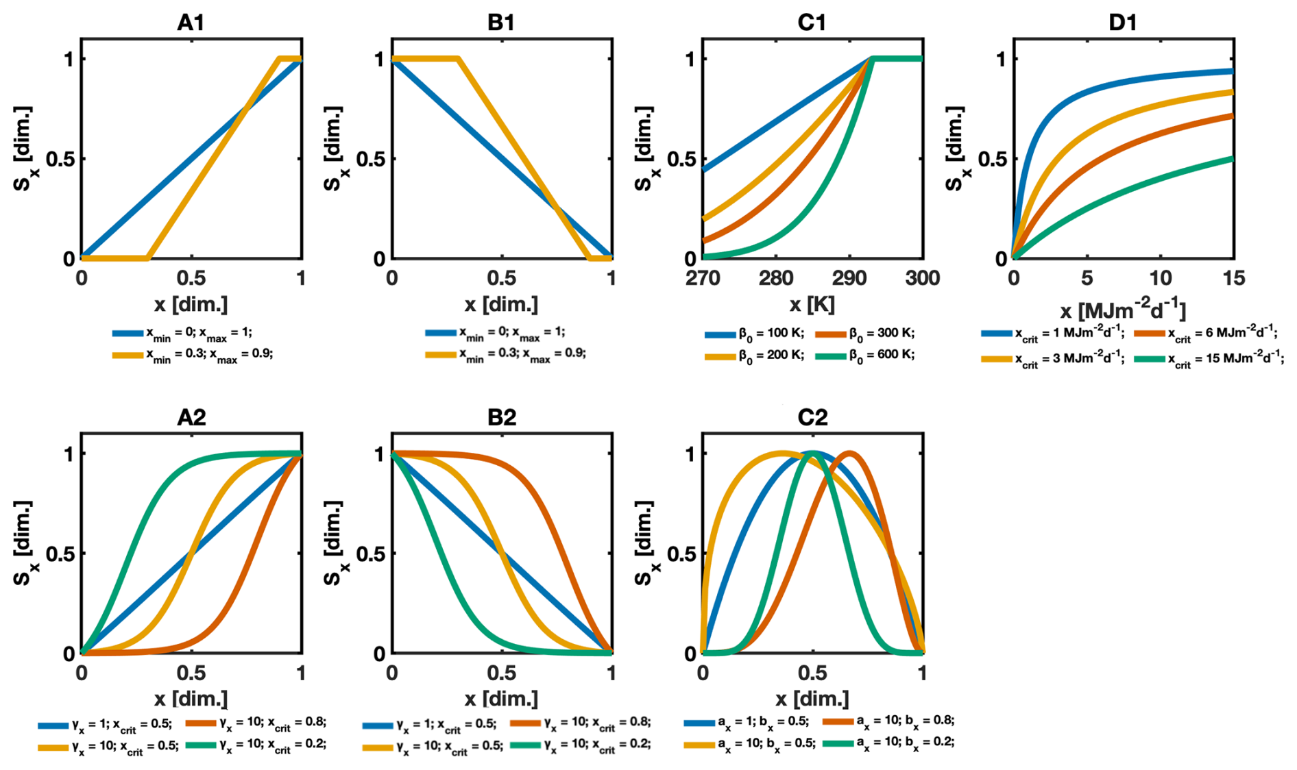
Figure B1Behavior of the ecosystem response functions used in the L4C model and the Arctic–Subarctic adapted formulations. Each panel shows the same response function evaluated across a range of parameter values to illustrate how parameterization affects function shape. Refer to Sects. 3 and 4.1 for a detailed description of each model formulation. Panels (A1), (B1), and (C1) correspond to Eq. (7a, c, d), (7b), and (7e), respectively; panel (D1) corresponds to Eq. (8b). Panels (A2) and (B2) correspond to Eq. (9a, c) and (9b), respectively; panel (C2) corresponds to Eqs. (10b) and (11).

Figure B2Mean seasonal cycle of daily averaged eddy covariance (EC) gross primary production (GPPEC) for upland tundra, taiga forests and wetlands. The horizontal red line indicates the estimated separation between dormant and transitional periods with active photosynthetic periods (i.e., the growing season) using a percentile-based GPPEC threshold (Sect. 4.2). This threshold corresponds to the mean 10th percentile computed across EC towers, with the 5th and 15th percentiles shown as variability bounds.
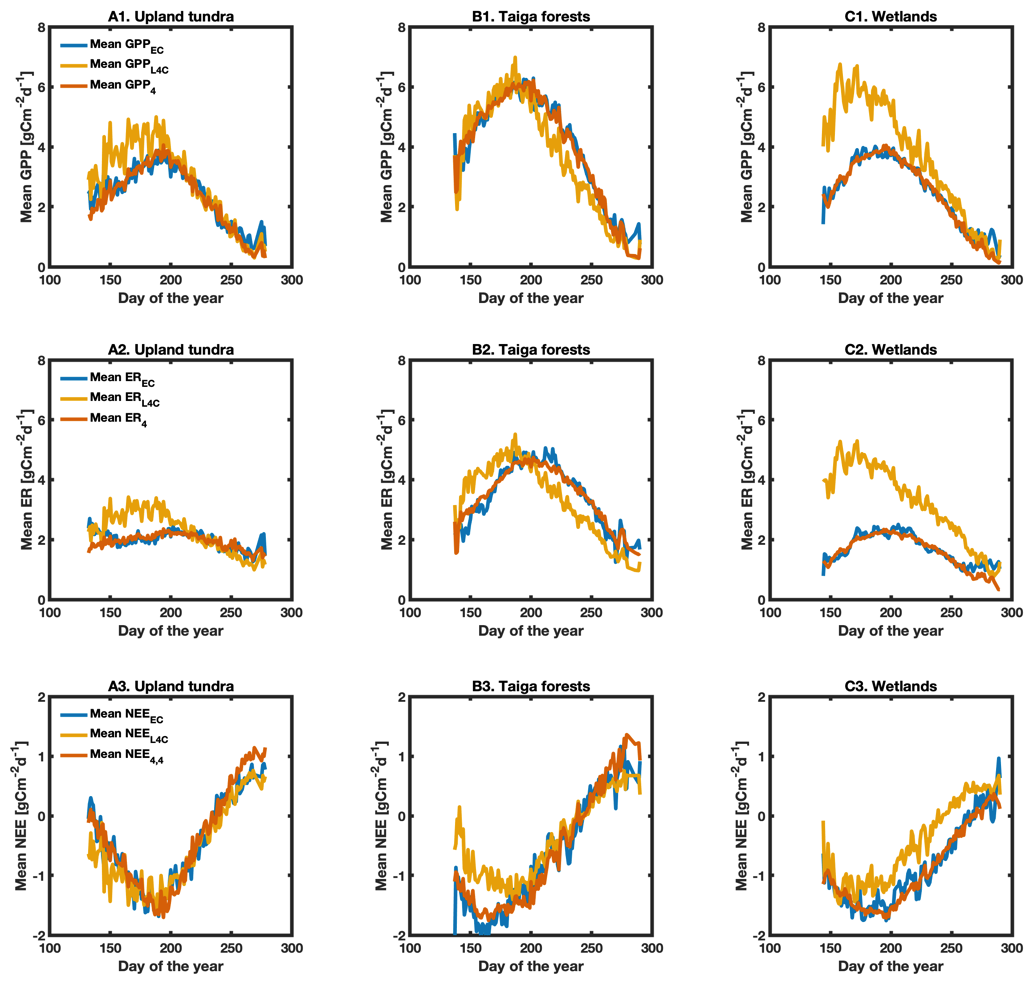
Figure B3Mean seasonal cycle of daily averaged gross primary production (GPP), ecosystem respiration (ER), and net ecosystem CO2 exchange (NEE) across eddy covariance tower sites for upland tundra, taiga forests, and wetlands. GPPEC, EREC, and NEEEC denote eddy covariance data. GPPL4C, ERL4C, and NEEL4C represent outputs from the original L4C model, whereas GPP4, ER4, and NEE4,4 (i.e., ER4 − GPP4) correspond to outputs from the Arctic–Subarctic adapted formulations using test case 4 for both GPP and ER (Sects. 3 and 4.1). The data shown represent the growing season after applying the filtering criteria described in Sect. 4.2.
Table C1Median differences in Akaike Information Criterion (AIC) and Bayesian Information Criterion (BIC) between GPP1 through GPP5 and GPPL4C. GPPL4C refers to GPP outputs from the original L4C model, while GPP1 through GPP5 represent the five Arctic–Subarctic (AS) adapted formulations (Sects. 3 and 4.1).
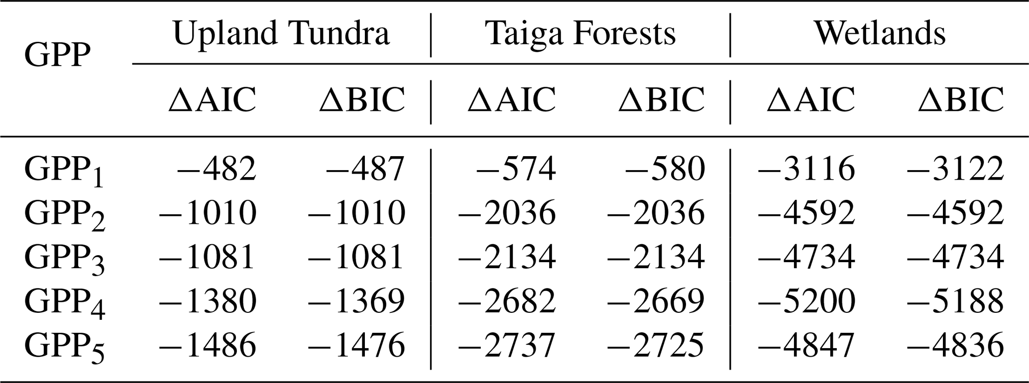
Table C2Same as Table 4, but here GPP4 and GPP5 use growing degree days (GDD) as inputs, which were normalized by the long-term minimum and maximum across all years rather than by annual values (Sect. 6.1).
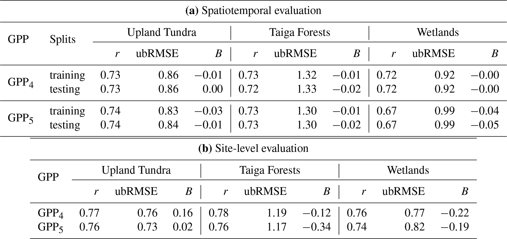
Table C3Same as Table 4, but instead of 100 runs with 70 %–30 % training–testing splits, the data were split into 6-year training and 2-year testing periods. The period of study spans a total of 8 years, yielding 28 possible runs instead of 100.
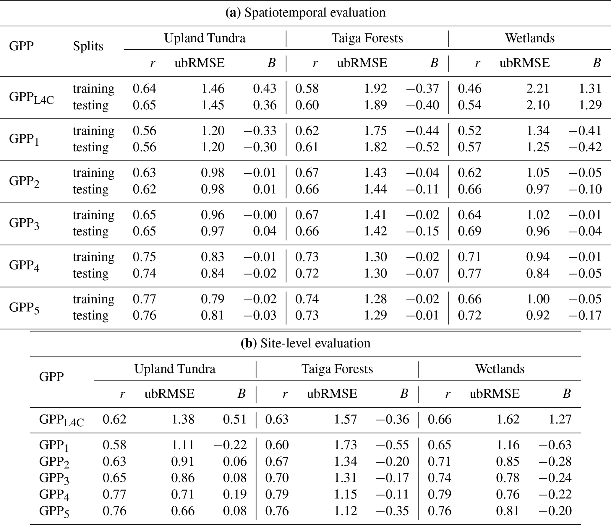
Table C4Same as Table 4, but the 70 %–30 % training-testing splits were applied to the set of eddy covariance (EC) tower sites rather than to the individual data points, such that all data from a given site were assigned to either the training or the testing split. Because the number of EC tower sites differs among ecosystems, this yielded 5, 21, and 28 possible runs for upland tundra, taiga forests, and wetlands, respectively, instead of 100.
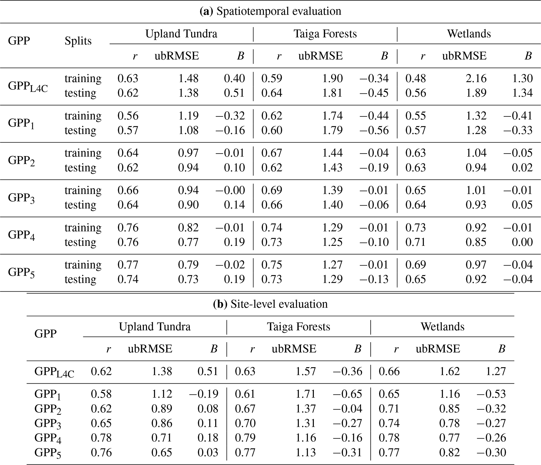
Table D1Same as Table 4, but for ecosystem respiration (ER). GPP1 was used as the GPP input for ER1 through ER5.
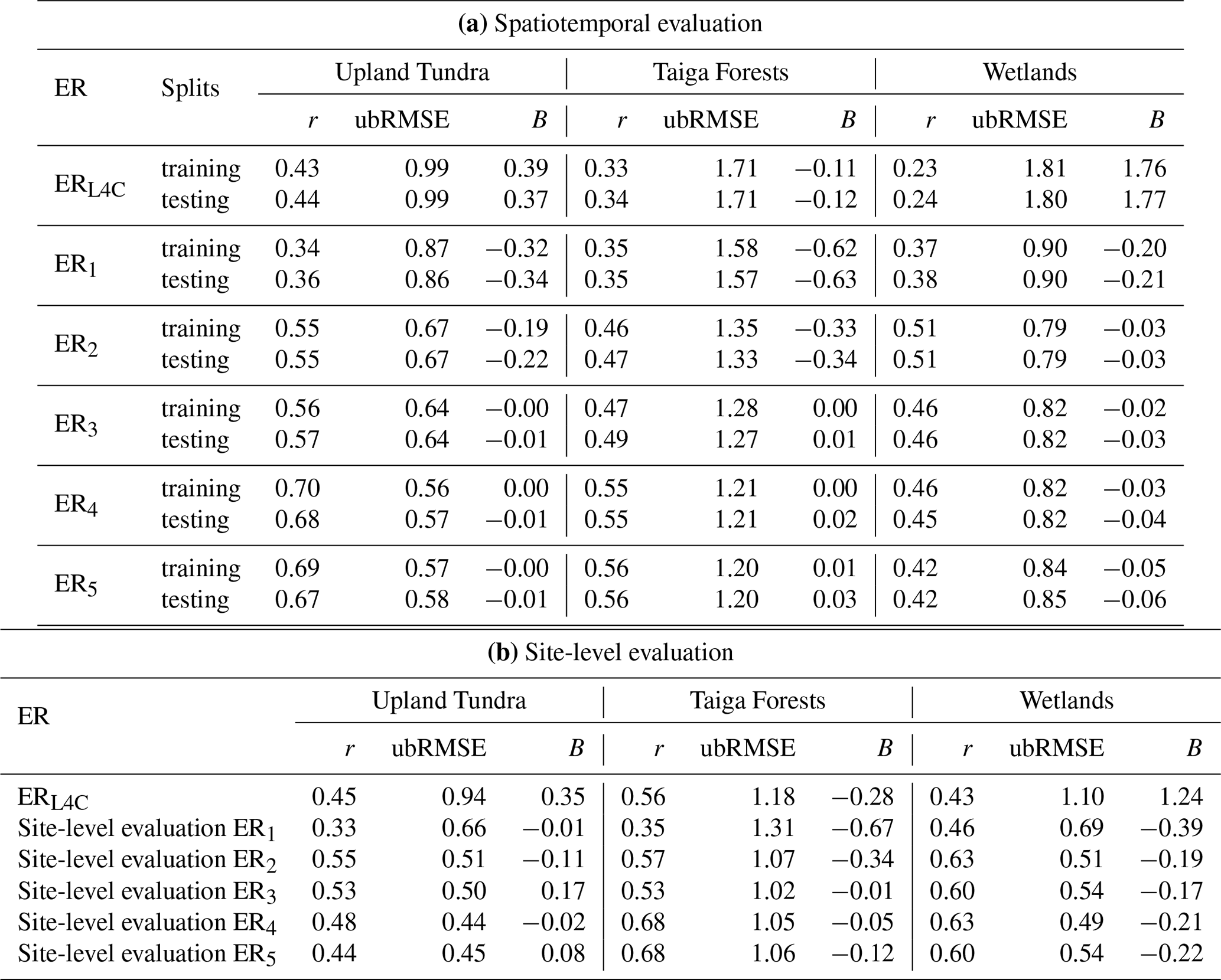
Table D2Same as Table 4, but for ecosystem respiration (ER). GPP2 was used as the GPP input for ER1 through ER5.
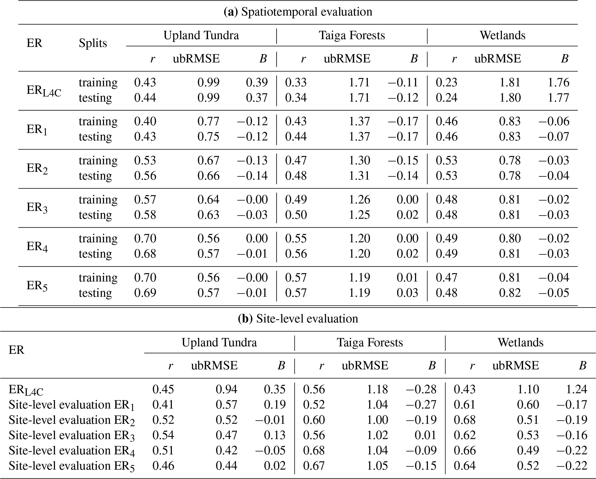
Table D3Same as Table 4, but for ecosystem respiration (ER). GPP3 was used as the GPP input for ER1 through ER5.
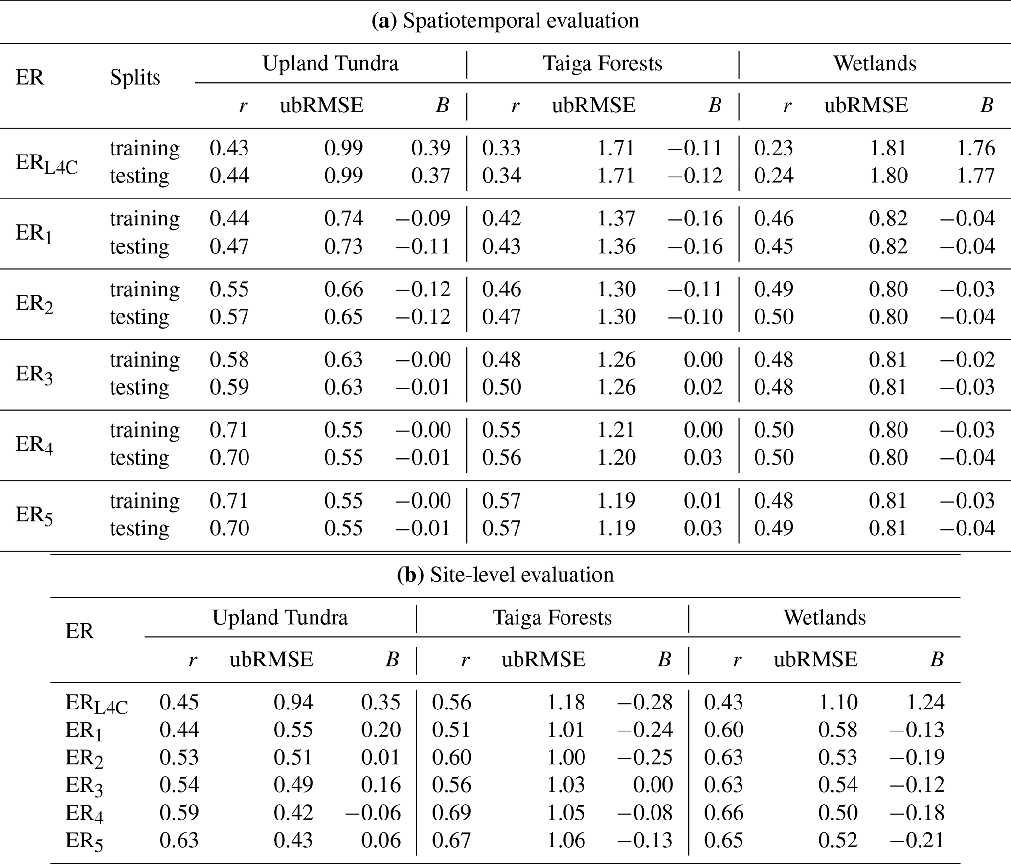
Table D4Same as Table 4, but for ecosystem respiration (ER). GPP4 was used as the GPP input for ER1 through ER5.
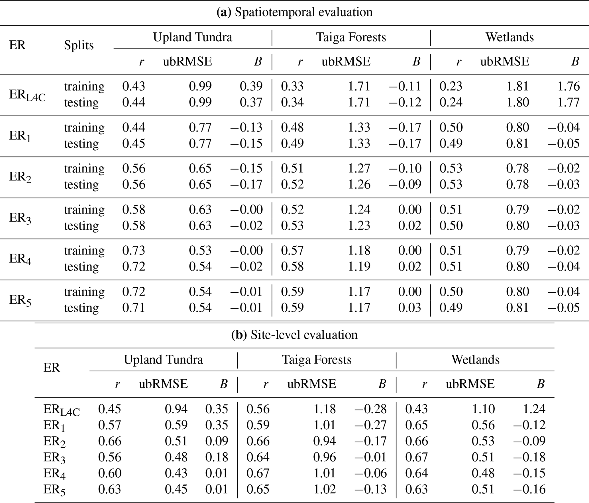
Table D5Same as Table 4, but for ecosystem respiration (ER). GPP5 was used as the GPP input for ER1 through ER5.
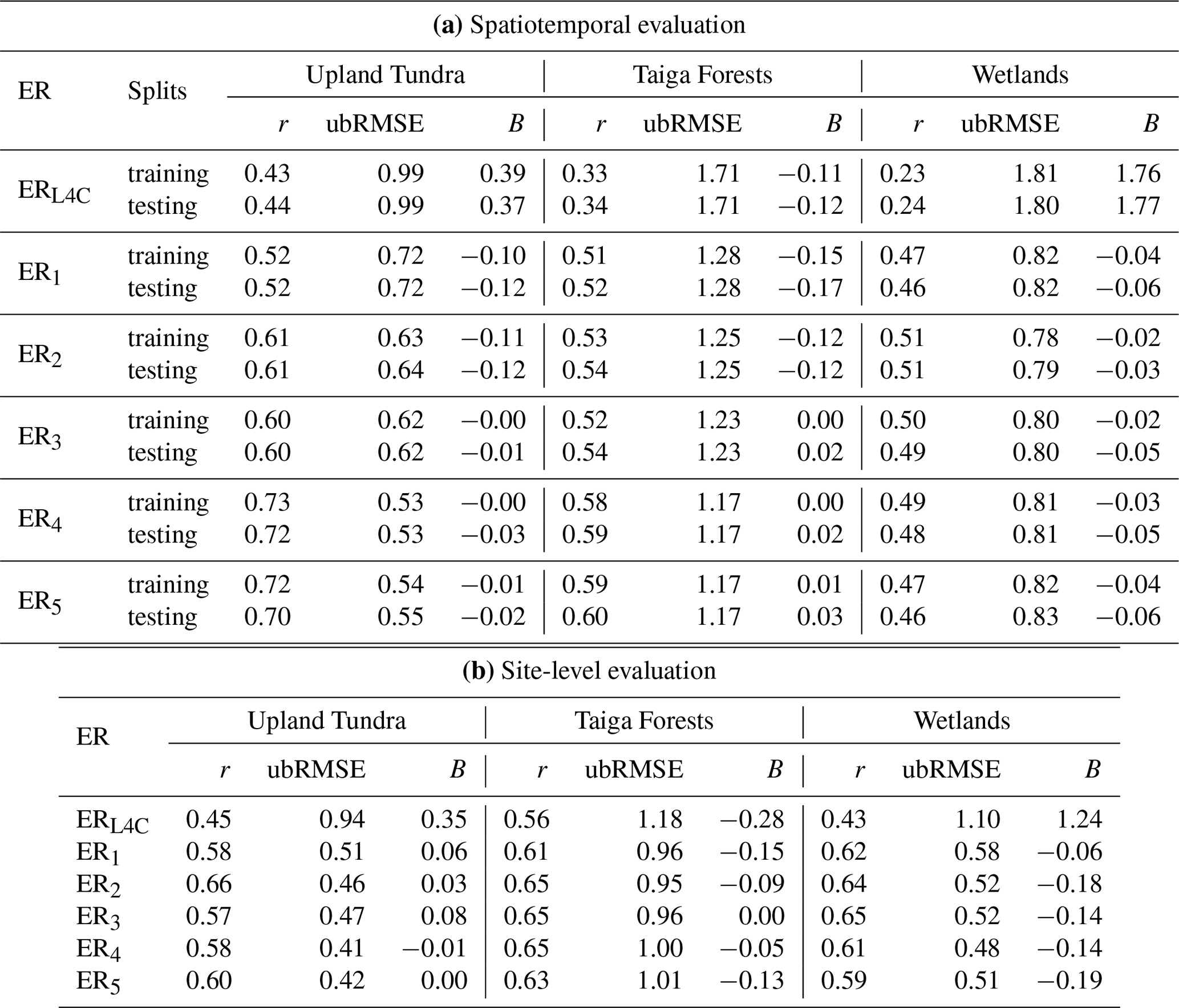
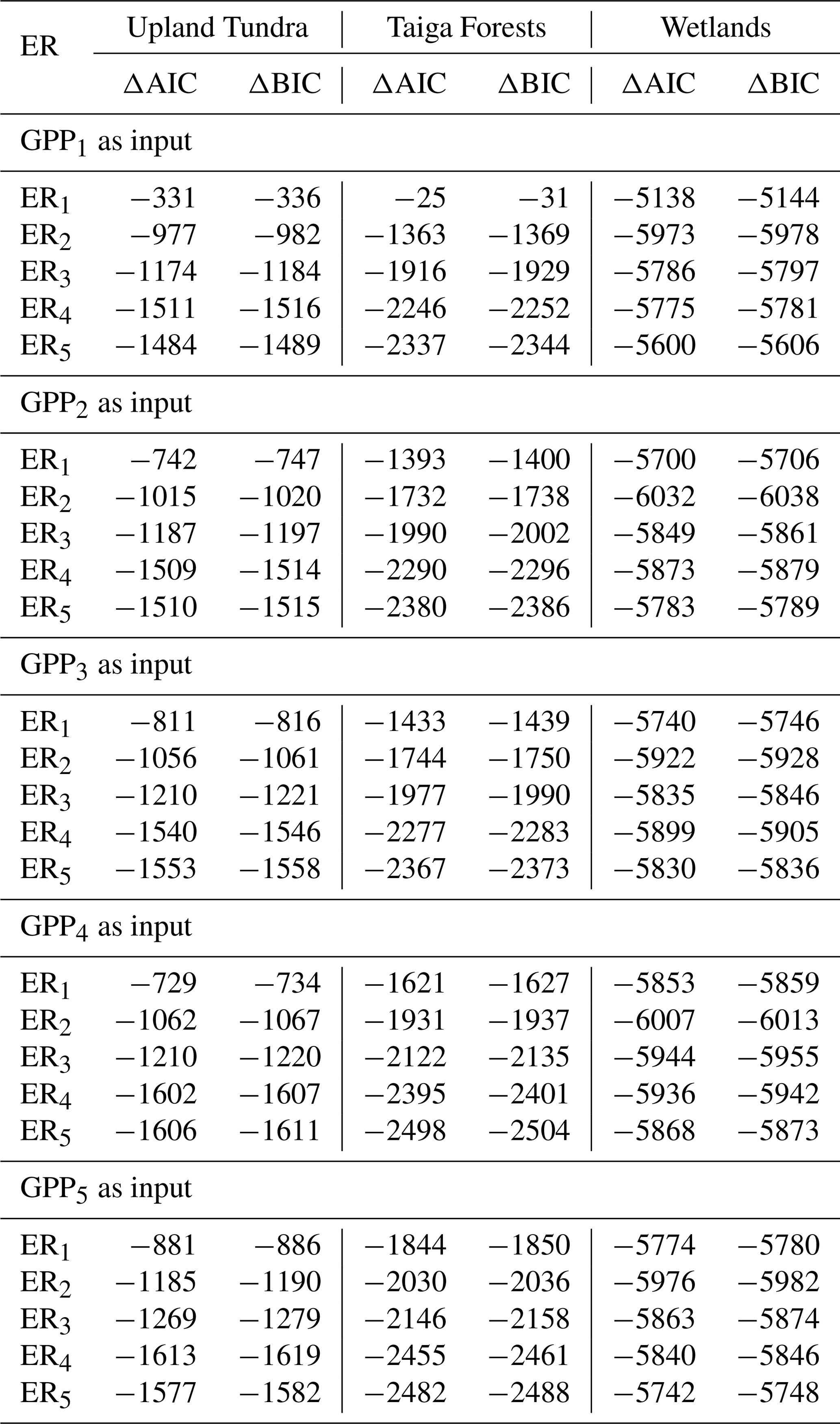
Table D7Same as Table 5, but instead of 100 runs with 70 %–30 % training–testing splits, the data were split into 6-year training and 2-year testing periods. The period of study spans a total of 8 years, yielding 28 possible runs instead of 100.
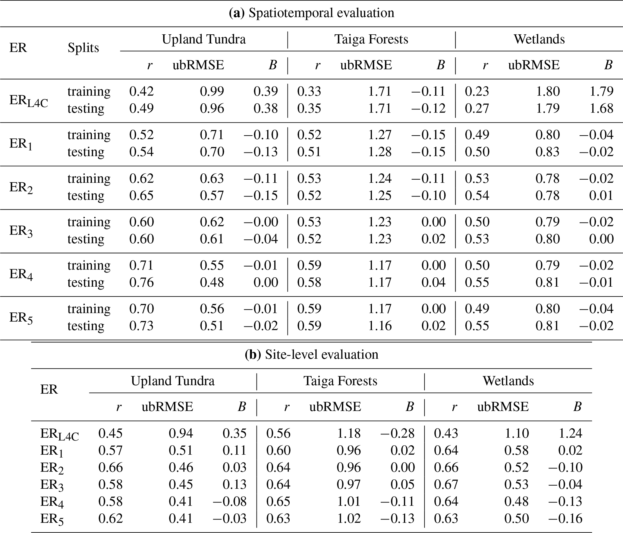
Table D8Same as Table 5, but the 70 %–30 % training-testing splits were applied to the set of eddy covariance (EC) tower sites rather than to the individual data points, such that all data from a given site were assigned to either the training or the testing split. Because the number of EC tower sites differs among ecosystems, this yielded 5, 21, and 28 possible runs for upland tundra, taiga forests, and wetlands, respectively, instead of 100.
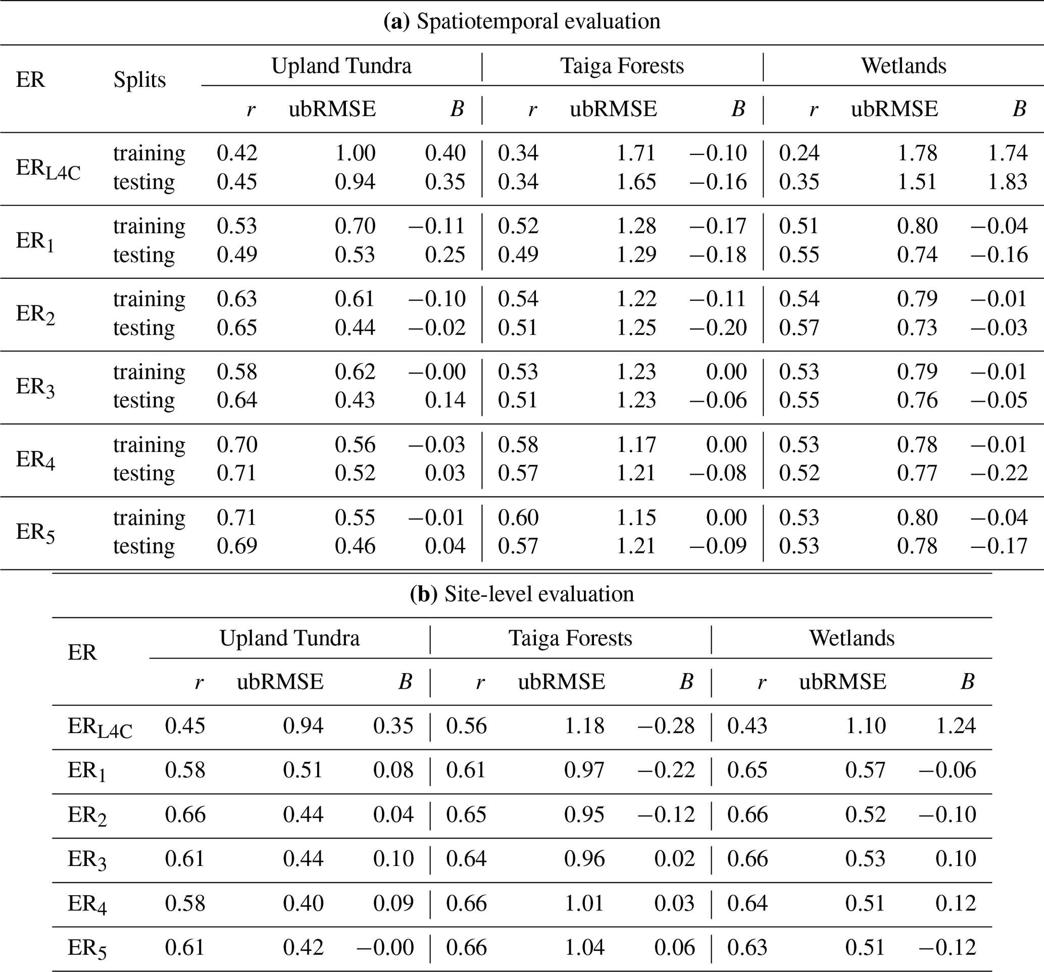
Table E1Same as Table 4, but for net ecosystem CO2 exchange (NEE). Modeled NEE is computed as the difference between modeled ecosystem respiration (ER) and gross primary production (GPP). NEEL4C denotes NEE from the original L4C model, while NEEi, 1 refers to outputs from the Arctic–Subarctic (AS) adapted ERi and GPP1 formulations.
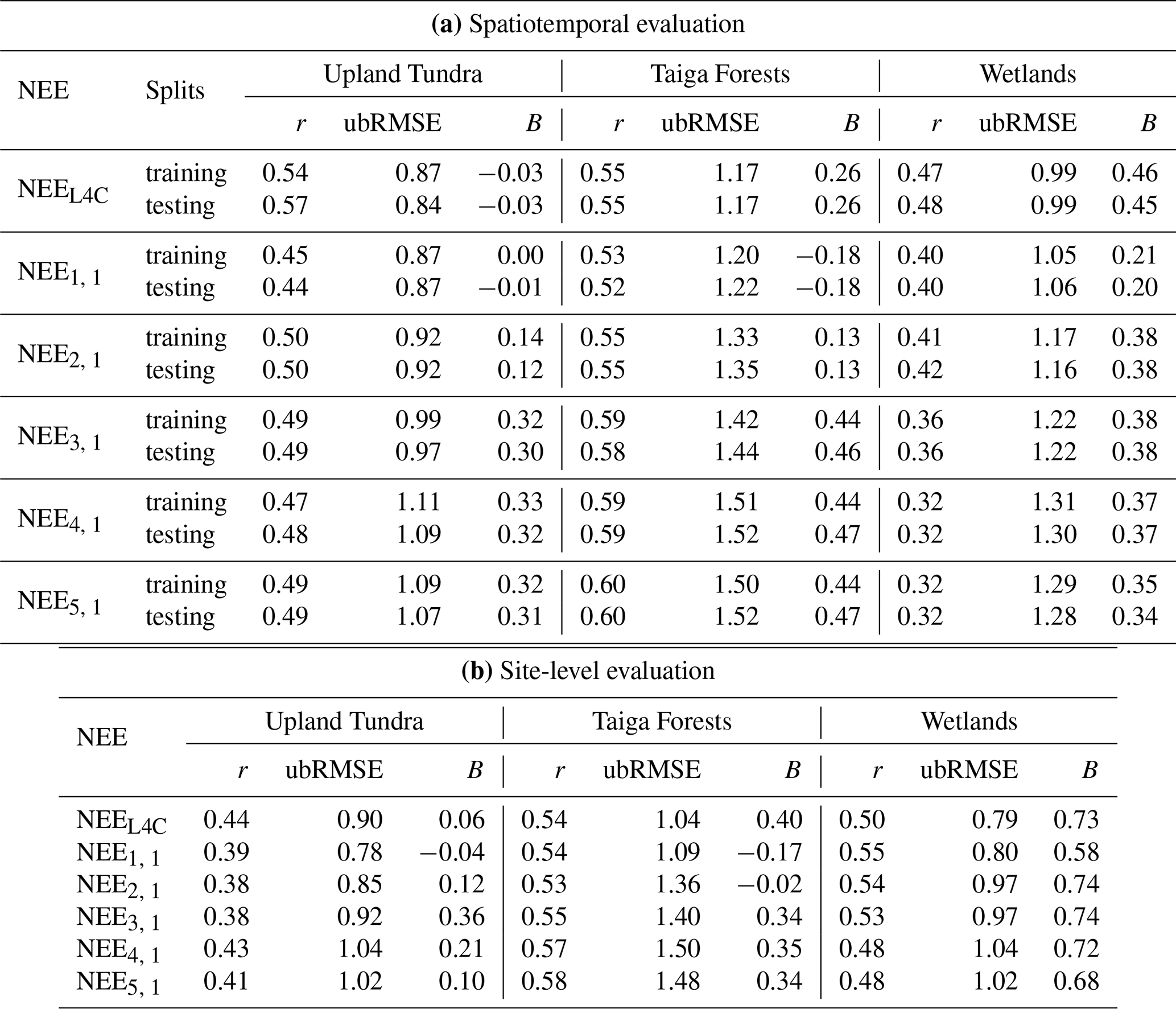
Table E2Same as Table 4, but for net ecosystem CO2 exchange (NEE). Modeled NEE is computed as the difference between modeled ecosystem respiration (ER) and gross primary production (GPP). NEEL4C denotes NEE from the original L4C model, while NEEi, 2 refers to outputs from the Arctic–Subarctic (AS) adapted ERi and GPP2 formulations.
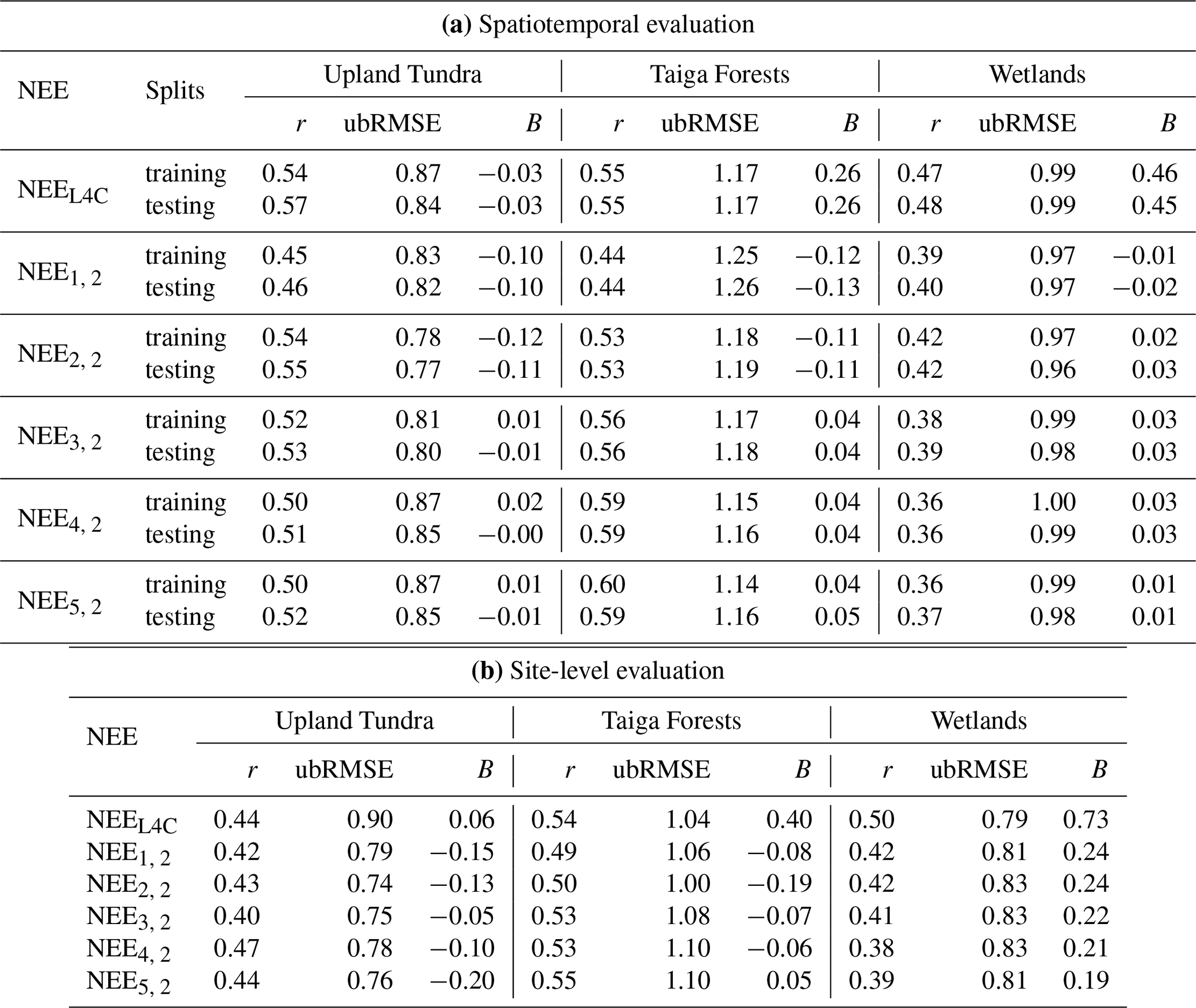
Table E3Same as Table 4, but for net ecosystem CO2 exchange (NEE). Modeled NEE is computed as the difference between modeled ecosystem respiration (ER) and gross primary production (GPP). NEEL4C denotes NEE from the original L4C model, while NEEi, 3 refers to outputs from the Arctic–Subarctic (AS) adapted ERi and GPP3 formulations.
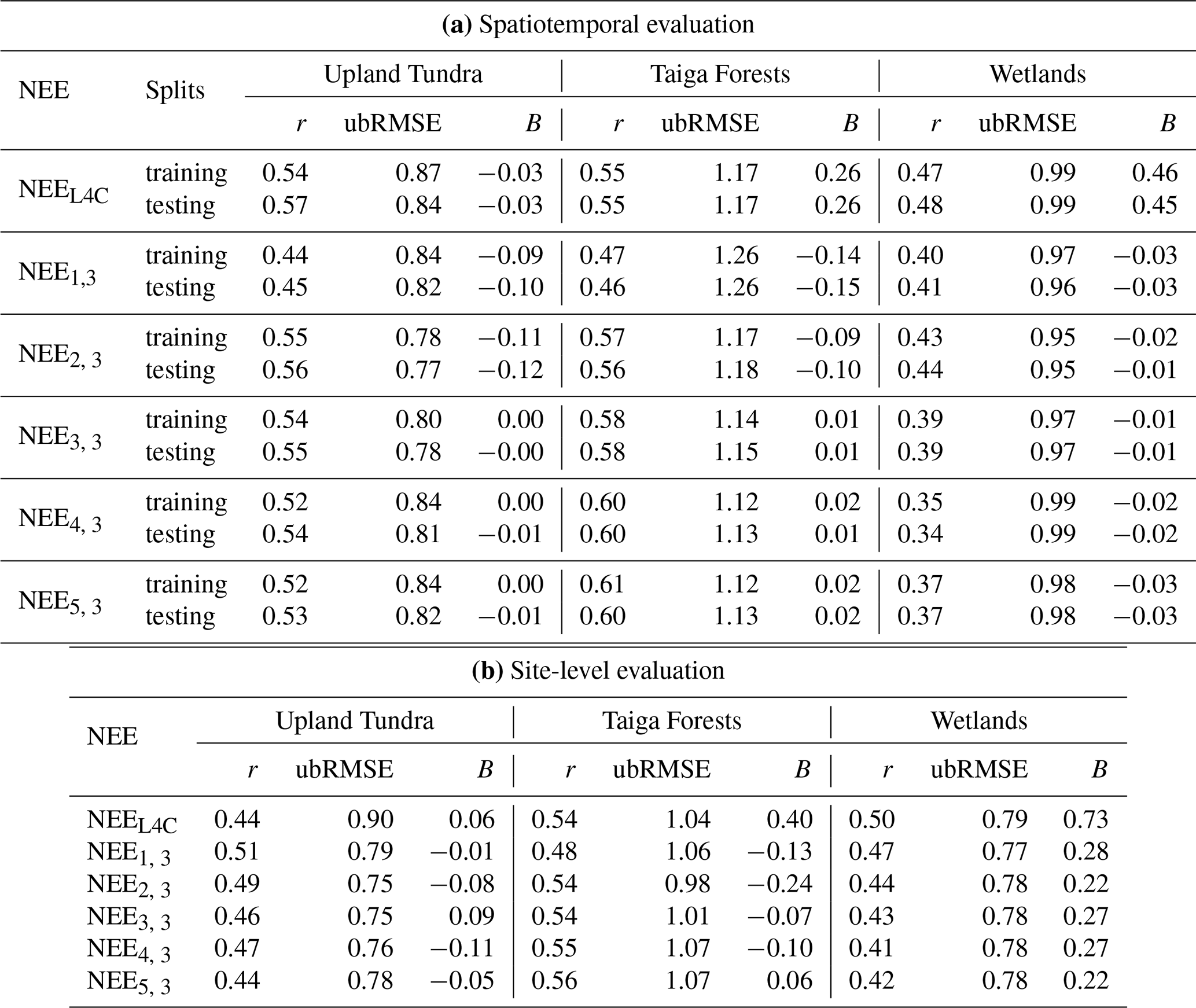
Table E4Same as Table 4, but for net ecosystem CO2 exchange (NEE). Modeled NEE is computed as the difference between modeled ecosystem respiration (ER) and gross primary production (GPP). NEEL4C denotes NEE from the original L4C model, while NEEi, 4 refers to outputs from the Arctic–Subarctic (AS) adapted ERi and GPP4 formulations.
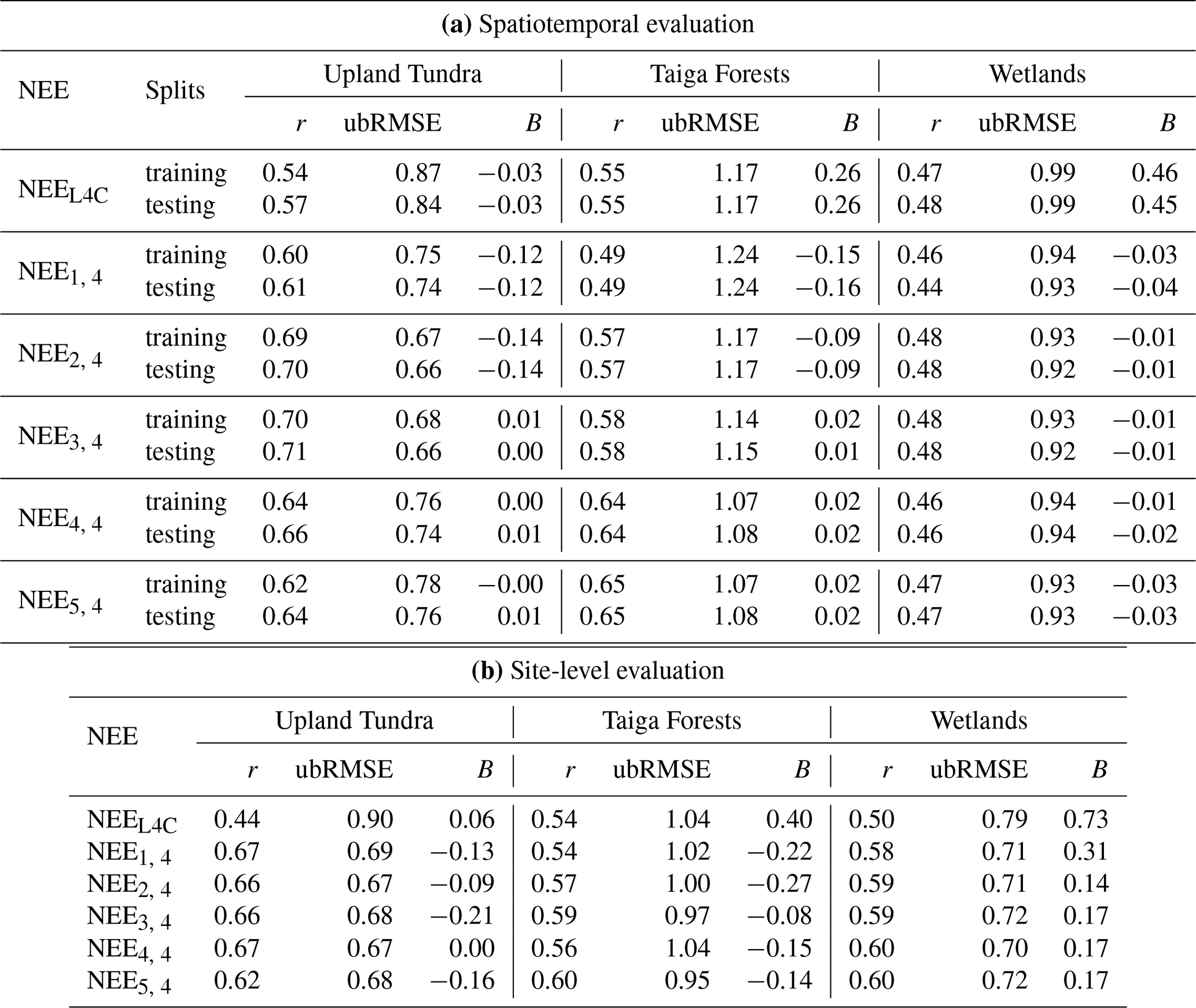
Table E5Same as Table 4, but for net ecosystem CO2 exchange (NEE). Modeled NEE is computed as the difference between modeled ecosystem respiration (ER) and gross primary production (GPP). NEEL4C denotes NEE from the original L4C model, while NEEi, 5 refers to outputs from the Arctic–Subarctic (AS) adapted ERi and GPP5 formulations.
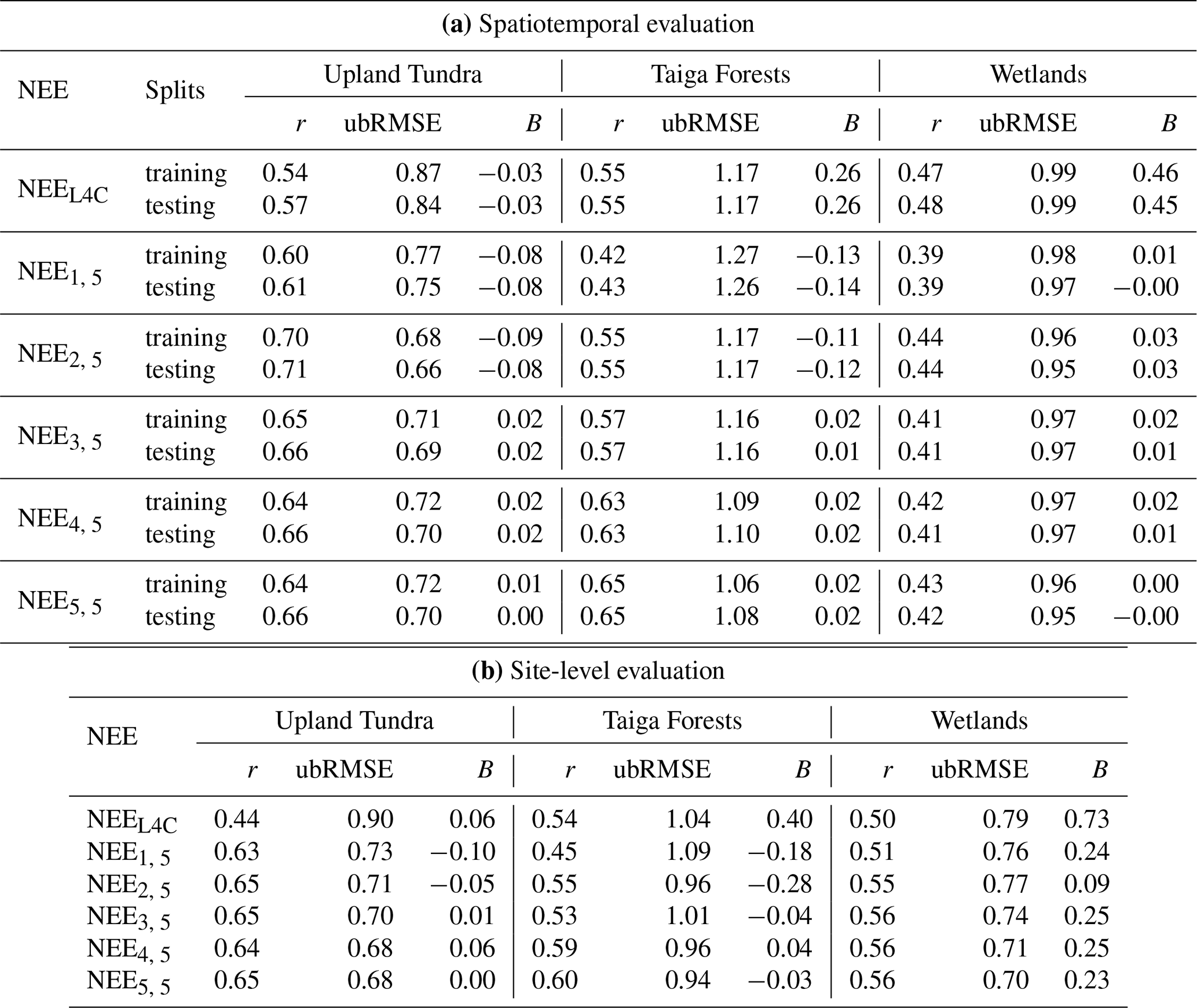
The SMAP SPL4CMDL Version 8 product can be downloaded from the National Snow and Ice Data Center (NSIDC) website at: https://doi.org/10.5067/U7SN8JDZL0UC (Kimball et al., 2025). The SMAP SPL4SMGP Version 8 product can be downloaded at: https://doi.org/10.5067/T5RUATAQREF8 (Reichle et al., 2025b). The MERRA-2 M2T1NXSLV Version 5.12.4 product is available at: https://goldsmr4.gesdisc.eosdis.nasa.gov/data/MERRA2/M2T1NXSLV.5.12.4/ (last access: 27 August 2025, Gelaro et al., 2017).
RM, ArM, and AR designed and conducted the study, and wrote the first draft of the manuscript. KAE and JSK provided scientific support throughout the study and contributed to the second version of the manuscript. OS, HA, SNW, AM provided some of the eddy covariance data. All authors contributed to the final version of the manuscript.
The contact author has declared that none of the authors has any competing interests.
Publisher's note: Copernicus Publications remains neutral with regard to jurisdictional claims made in the text, published maps, institutional affiliations, or any other geographical representation in this paper. The authors bear the ultimate responsibility for providing appropriate place names. Views expressed in the text are those of the authors and do not necessarily reflect the views of the publisher.
The research made use of eddy covariance data from the AmeriFlux network (https://ameriflux.lbl.gov, last access: August 21, 2025). Additional eddy covariance data were directly provided by the principal investigators O. Sonnentag and S. N. Williamson. We thank all the principal investigators and site teams of the eddy covariance tower sites (listed in Table 1) for their sustained efforts in site maintenance, data processing, and data sharing. All the authors thank the indigenous and northern communities for agreeing to the installation of eddy covariance towers on their territory. As a non-native English speaker, R. Madelon acknowledges the use of artificial intelligence tools to improve the writing quality of the manuscript. Finally, the authors acknowledge the constructive reviews from the referees, which have improved both the clarity of the manuscript and its content.
R. Madelon, A. Mialon and A. Roy acknowledge fundings from the Université of Toulouse 3 Paul Sabatier in France, and the Université du Québec à Trois-Rivières in Canada through the Universalis Causa, Samuel-de-Champlain, Programme d’Aide à L’Internationalisation de la Recherche (PAIR), Fonds Canadien de l’Innovation (FCI) and Conseil de Recherches en Sciences Naturelles et en Génie du Canada (CRSNG), and Fonds de recherche du Québec (FRQ) grants. J. S. Kimball and K. A. Endsley acknowledge fundings from NASA (grant no. NX14AI50G). G. De Lannoy acknowledges funding from KU Leuven C1 (C14/21/057). O. Sonnentag acknowledges financial support through the Canada Research Chair and NSERC Discovery Grants programs, ArcticNet, a Network of Centres of Excellence Canada, the Canada First Research Excellence Fund’s Global Water Futures program (Northern Water Futures), and the Polar Continental Shelf Program.
This paper was edited by Andrew Feldman and reviewed by Preet Lal and one anonymous referee.
Aubinet, M., Vesala, T., and Papale, D.: Eddy covariance: a practical guide to measurement and data analysis, Springer Science & Business Media, ISBN 978-94-007-2350-4, e-ISBN 978-94-007-2351-1, https://doi.org/10.1007/978-94-007-2351-1, 2012. a, b, c, d, e, f, g, h
Baldocchi, D., Falge, E., Gu, L., Olson, R., Hollinger, D., Running, S., Anthoni, P., Bernhofer, C., Davis, K., Evans, R., Fuentes, J., Goldstein, A., Katul, G., Law, B., Lee, X., Malhi, Y., Meyers, T., Munger, W., Oechel, W., Paw U, K., Pilegaard, K., Schmid, H., Valentini, R., Verma, S., Vesala, T., Wilson, K., and Wofsy, S.: FLUXNET: A New Tool to Study the Temporal and Spatial Variability of Ecosystem–Scale Carbon Dioxide, Water Vapor, and Energy Flux Densities, B. Am. Meteorol. Soc., 82, 2415–2434, https://doi.org/10.1175/1520-0477(2001)082<2415:FANTTS>2.3.CO;2, 2007. a
Bao, S., Wutzler, T., Koirala, S., Cuntz, M., Ibrom, A., Besnard, S., Walther, S., Šigut, L., Moreno, A., Weber, U., Wohlfahrt, G., Cleverly, J., Migliavacca, M., Woodgate, W., Merbold, L., Elmar, V., and Carvalhais, N.: Environment-sensitivity functions for gross primary productivity in light use efficiency models, Agr. Forest Meteorol., 312, 108708, https://doi.org/10.1016/j.agrformet.2021.108708, 2022. a
Bell, J., Palecki, M., Baker, C., Collins, W., Lawrimore, J., Leeper, R., Hall, M., Kochendorfer, J., Meyers, T., Wilson, T., and Diamond, H.: U.S. Climate Reference Network soil moisture and temperature observations., J. Hydrometeorol., 14, 977–988, 2013. a
Blume-Werry, G., Milbau, A., Teuber, L. M., Johansson, M., and Dorrepaal, E.: Dwelling in the deep–strongly increased root growth and rooting depth enhance plant interactions with thawing permafrost soil, New Phytol., 223, 1328–1339, 2019. a
Bowling, D. R., Logan, B. A., Hufkens, K., Aubrecht, D. M., Richardson, A. D., Burns, S. P., Anderegg, W. R. L., Blanken, P. D., and Eiriksson, D. P.: Limitations to winter and spring photosynthesis of a Rocky Mountain subalpine forest, Agr. Forest Meteorol., 252, 241–255, 2018. a
Bracho, R., Celis, G., Rodenhizer, H., See, C., and Schuur, E. A.: AmeriFlux BASE US-EML Eight Mile Lake Permafrost thaw gradient, Healy Alaska, Ver. 4-5, AmeriFlux AMP [data set], https://doi.org/10.17190/AMF/1418678, 2021. a
Brown, J., Ferrians, O., Heginbottom, J., and Melnikov, E.: Circum-Arctic Map of Permafrost and Ground-Ice Conditions, Version 2, National Snow and Ice Data Center [data set], https://doi.org/10.7265/skbg-kf16, 2002. a
Burba, G.: Eddy Covariance Method for Scientific, Industrial, Agricultural and Regulatory Applications: A Field Book on Measuring Ecosystem Gas Exchange and Areal Emission Rates, LI-COR Biosciences, Lincoln, NE, USA, 331 pp., ISBN 978-0-615-76827-4, 2013. a
Burba, G.: Eddy Covariance Method for Scientific, Regulatory, and Commercial Applications, LI-COR Biosciences, Lincoln, NE, USA, 702 pp., ISBN 978-0-578-97714-0. a, b
Chapin, F., Woodwell, G., Randerson, J., Rastetter, E., Lovett, G., Baldocchi, D., Clark, D., Harmon, M., Schimel, D., Valentini, R., Wirth, C., Aber, J., Cole, J., Goulden, M., Harden, J., Heimann, M., Howarth, R., Matson, P., McGuire, A., Melillo, J., Mooney, H., Neff, J., Houghton, R., Pace, M., Ryan, M., Running, S., Sala, O., Schlesinger, W., and Schulze, E.-D.: Reconciling Carbon-cycle Concepts, Terminology, and Methods., Ecosystems, 9, 1041–1050, 2006. a
Chen, N., Zhang, Y., Yuan, F., Song, C., Xu, M., Wang, Q., Hao, G., Bao, T., Zuo, Y., Liu, J., Song, Y., Sun, L., Guo, Y., Zhang, H., Ma, G., Du, Y., Xu, X., and Wang, X.: Warming-induced vapor pressure deficit suppression of vegetation growth diminished in northern peatlands, Nat. Commun., 14, 7885, https://doi.org/10.1038/s41467-023-42932-w, 2023. a
Churchill, A. C., Turetsky, M. R., McGuire, A. D., and Hollingsworth, T. N.: Response of plant community structure and primary productivity to experimental drought and flooding in an Alaskan fen, Can. J. Forest Res., 45, 185–193, 2015. a
Colliander, A., Jackson, T., Bindlish, R., Chan, S., Das, N., Kim, S., Cosh, M., Dunbar, R., Dang, L., Pashaian, L., Asanuma, J., Aida, K., Berg, A., Rowlandson, T., Bosch, D., Caldwell, T., Caylor, K., Goodrich, D., al Jassar, H., Lopez-Baeza, E., Martínez Fernández, J., González-Zamora, A., Livingston, S., McNairn, H., Pacheco, A., Moghaddam, M., Montzka, C., Notarnicola, C., Niedrist, G., Pellarin, T., Prueger, J., Pulliainen, J., Rautiainen, K., Ramos, J., Seyfried, M., Starks, P., Su, Z., Zeng, Y., van der Velde, R., Thibeault, M., Dorigo, W., Vreugdenhil, M., Walker, J. P., Wu, X., Monerris, A., O'Neill, P. E., Entekhabi, D., Njoku, E., and Yueha, S.: Validation of SMAP surface soil moisture products with core validation sites, Remote Sens. Environ., 191, 215–231, 2017. a
Crawford, R. M. M.: Tundra-taiga biology, Oxford University Press, ISBN 978-0-19-955940-4, 2013. a, b, c
Davis, T. W., Prentice, I. C., Evans, B. J., Wang, H., and Gilbert, X.: The Global ecosystem Production in Space and Time (GePiSaT) Model of the Terrestrial Biosphere, 2014 AGU Fall Meeting, abstract H53J-04, San Francisco, CA, USA, December 2014. a, b
Derksen, C., Xu, X., Scott Dunbar, R., Colliander, A., Kim, Y., Kimball, J. S., Black, T. A., Euskirchen, E., Langlois, A., Loranty, M. M., Marsh, P.cand Rautiainen, K., Roy, A., Royer, A., and Stephens, J.: Retrieving landscape freeze/thaw state from Soil Moisture Active Passive (SMAP) radar and radiometer measurements, Remote Sens. Environ., 194, 48–62, 2017. a
Dragoni, D., Schmid, H. P., Grimmond, C. S. B., and Loescher, H. W.: Uncertainty of annual net ecosystem productivity estimated using eddy covariance flux measurements, J. Geophys. Res.-Atmos., 112, https://doi.org/10.1029/2006JD008149, 2007. a
Elmendorf, S. C. and Hollister, R. D.: Limits on phenological response to high temperature in the Arctic, Scientific Reports, 13, 208, https://doi.org/10.1038/s41598-022-26955-9, 2023. a
Endsley, K., Kimball, J., and Reichle, R.: Soil respiration phenology improves modeled phase of terrestrial net ecosystem exchange in northern hemisphere, J. Adv. Model. Earth Sy., 14, e2021MS002804, https://doi.org/10.1029/2021MS002804, 2022. a, b, c, d, e, f
Ensminger, I., Sveshnikov, D., Campbell, D. A., Funk, C., Jansson, S., Lloyd, J., Shibistova, O., and Öquist, G.: Intermittent low temperatures constrain spring recovery of photosynthesis in boreal Scots pine forests, Glob. Change Biol., 10, 995–1008, 2004. a
Entekhabi, D., Njoku, E. G., O'Neill, P. E., Kellogg, K. H., Crow, W. T., Edelstein, W. N., Entin, J. K., Goodman, S. D., Jackson, T. J., Johnson, J., Kimball, J., Piepmeier, J. R., Koster, R. D., Martin, N., McDonald, K. C., Moghaddam, M., Moran, S., Reichle, R., Shi, J. C., Spencer, M. W., Thurman, S. W., Tsang, L., and Van Zyl, J.: The soil moisture active passive (SMAP) mission, P. IEEE, 98, 704–716, 2010. a
Entekhabi, D., Yueh, S., O’Neill, P. E., and Kellogg, K. H.: SMAP Handbook, Tech. rep., Jet Propulsion Laboratory, NASA, https://smap.jpl.nasa.gov/files/smap2/SMAP_Handbook_FINAL_1_JULY_2014_Web.pdf (last access: 29 June 2023), 2014. a
Eugster, W., McFadden, J. P., and Chapin, F. S.: A comparative approach to regional variation in surface fluxes using mobile eddy correlation towers, Bound.-Lay. Meteorol., 85, 293–307, 1997. a
Euskirchen, E.: AmeriFlux BASE US-BZB Bonanza Creek Thermokarst Bog, Ver. 4-5, AmeriFlux AMP [data set], https://doi.org/10.17190/AMF/1773401, 2022a. a
Euskirchen, E.: AmeriFlux BASE US-BZF Bonanza Creek Rich Fen, Ver. 4-5, AmeriFlux AMP [data set], https://doi.org/10.17190/AMF/1756433, 2022b. a
Euskirchen, E.: AmeriFlux BASE US-BZo Bonanza Creek Old Thermokarst Bog, Ver. 3-5, AmeriFlux AMP [data set], https://doi.org/10.17190/AMF/1846662, 2022c. a
Euskirchen, E.: AmeriFlux BASE US-BZS Bonanza Creek Black Spruce, Ver. 3-5, AmeriFlux AMP [data set], https://doi.org/10.17190/AMF/1756434, 2022d. a
Euskirchen, E., Shaver, G., and Bret-Harte, S.: AmeriFlux BASE US-ICh Imnavait Creek Watershed Heath Tundra, Ver. 4-5, AmeriFlux AMP [data set], https://doi.org/10.17190/AMF/1246133, 2022a. a
Euskirchen, E., Shaver, G., and Bret-Harte, S.: AmeriFlux BASE US-ICs Imnavait Creek Watershed Wet Sedge Tundra, Ver. 7-5, AmeriFlux AMP [data set], https://doi.org/10.17190/AMF/1246130, 2022b. a
Euskirchen, E., Shaver, G., and Bret-Harte, S.: AmeriFlux BASE US-ICt Imnavait Creek Watershed Tussock Tundra, Ver. 5-5, AmeriFlux AMP [data set], https://doi.org/10.17190/AMF/1246131, 2022c. a
Euskirchen, E. S., McGuire, A. D., Chapin III, F. S., Yi, S., and Thompson, C. C.: Changes in vegetation in northern Alaska under scenarios of climate change, 2003–2100: implications for climate feedbacks, Ecol. Appl., 19, 1022–1043, 2009. a
Falge, E., Baldocchi, D., Olson, R., Anthoni, P., Aubinet, M., Bernhofer, C., Burba, G., Ceulemans, R., Clement, R., Dolman, H., and Granier, A.: Gap filling strategies for defensible annual sums of net ecosystem exchange, Agr. Forest Meteorol., 107, 43–69, 2001. a, b
Finkelstein, P. L. and Sims, P. F.: Sampling error in eddy correlation flux measurements, J. Geophys. Res.-Atmos., 106, 3503–3509, 2001. a
Fisher, J. B., Hayes, D. J., Schwalm, C. R., Huntzinger, D. N., Stofferahn, E., Schaefer, K.and Luo, Y., Wullschleger, S. D., Goetz, S., Miller, C. E., Griffith, P., Chadburn, S., Chatterjee, A., Ciais, P., Douglas, T., Genet, H., Ito, A., Neigh, C., Poulter, B., Rogers, B., Sonnentag, O., Tian, H., Wang, W., Xue, Y., Yang, Z.-L., Zeng, N., , and Zhang, Z.: Missing pieces to modeling the Arctic-Boreal puzzle, Environ. Res. Lett., 13, 020202, https://doi.org/10.1088/1748-9326/aa9d9a, 2018. a, b, c, d
Forkel, M., Carvalhais, N., Rödenbeck, C., Keeling, R., Heimann, M., Thonicke, K., Zaehle, S., and Reichstein, M.: Enhanced seasonal CO2 exchange caused by amplified plant productivity in northern ecosystems, Science, 351, 696–699, 2016. a
Foster, K. T., Sun, W., Merder, J., Kurz, W. A., Sinha, E., Nesdoly, A., Metsaranta, J., Hararuk, O., Bond-Lamberty, B. P., Schwalm, C., Natali, S. M., Huntzinger, D. N., and Michalak, A. M.: Permafrost, Peatland and Agricultural Regions Key to Reconciling Top-Down and Bottom-Up Estimates of North American Carbon Uptake, 2024 AGU Fall Meeting, abstract A43T-08, Washington, DC, USA, December 2024. a
Fotouo Makouate, H. and Zude-Sasse, M.: Advances in Growing Degree Days Models for Flowering to Harvest: Optimizing Crop Management with Methods of Precision Horticulture – A Review, Horticulturae, 11, 1415, https://doi.org/10.3390/horticulturae11121415, 2025. a
Friedl, M. and Sulla-Menashe, D.: MCD12Q1 MODIS/Terra+Aqua Land Cover Type Yearly L3 Global 500m SIN Grid V006, NASA Land Processes Distributed Active Archive Center [data set], https://doi.org/10.5067/MODIS/MCD12Q1.006, 2019. a, b
Fu, Y. H., Piao, S., Zhao, H., Jeong, S.-J., Wang, X., Vitasse, Y., Ciais, P., and Janssens, I. A.: Unexpected role of winter precipitation in determining heat requirement for spring vegetation green-up at northern middle and high latitudes, Glob. Change Biol., 20, 3743–3755, 2014. a
Gelaro, R., McCarty, W., Suárez, M. J., Todling, R., Molod, A., Takacs, L., Randles, C. A., Darmenov, A., Bosilovich, M. G., Reichle, R., Wargan, K., Coy, L., Cullather, R., Draper, C., Akella, S., Buchard, V., Conaty, A., da Silva, A. M., Gu, W., Kim, G.-K., Koster, R., Lucchesi, R., Merkova, D., Nielsen, J. E., Partyka, G., Pawson, S., Putman, W., Rienecker, M., Schubert, S. D., Sienkiewicz, M., and Zhao, B.: The modern-era retrospective analysis for research and applications, version 2 (MERRA-2), J. Climate, 30, 5419–5454, 2017. a, b
Gilmanov, T. G., Verma, S. B., Sims, P. L., Meyers, T. P., Bradford, J. A., Burba, G. G., and Suyker, A. E.: Gross primary production and light response parameters of four Southern Plains ecosystems estimated using long-term CO2-flux tower measurements, Global Biogeochem. Cy., 17, https://doi.org/10.1029/2002GB002023, 2003. a
Gonsamo, A., Chen, J. M., and D’Odorico, P.: Deriving land surface phenology indicators from CO2 eddy covariance measurements, Ecol. Indic., 29, 203–207, 2013. a
Hagedorn, F., Imboden, J., Moiseev, P. A., Gao, D., Frossard, E., Schleppi, P., Christen, D., Gavazov, K., and Fetzer, J.: Distinct changes in carbon, nitrogen, and phosphorus cycling in the litter layer across two contrasting forest–tundra ecotones, Biogeosciences, 22, 2959–2977, https://doi.org/10.5194/bg-22-2959-2025, 2025. a
Hayes, D. J., McGuire, A. D., Kicklighter, D. W., Gurney, K. R., Burnside, T., and Melillo, J. M.: Is the northern high-latitude land-based CO2 sink weakening?, Global Biogeochem. Cy., 25, https://doi.org/10.1029/2010GB003813, 2011. a
He, H., Moore, T., Lafleur, P., Sonnentag, O., Humphreys, E., Wu, M., and Roulet, N.: Spring phenology in photosynthesis control and modeling for a temperate bog, Frontiers in Environmental Science, 13, 1548578, https://doi.org/10.3389/fenvs.2025.1548578, 2025. a
Heinzelmann, V., Marinissen, J., Aerts, R., Cornelissen, J. H. C., and Bokhorst, S.: Stronger Drought Response of CO2 Fluxes in Tundra Heath Compared to Sphagnum Peatland in the Sub-Arctic, Glob. Change Biol., 31, e70210, https://doi.org/10.1111/gcb.70210, 2025. a
Helbig, M., Chasmer, L. E., Desai, A. R., Kljun, N., Quinton, W. L., and Sonnentag, O.: Direct and indirect climate change effects on carbon dioxide fluxes in a thawing boreal forest–wetland landscape, Glob. Change Biol., 23, 3231–3248, 2017a. a, b, c, d
Helbig, M., Chasmer, L. E., Kljun, N., Quinton, W. L., Treat, C. C., and Sonnentag, O.: The positive net radiative greenhouse gas forcing of increasing methane emissions from a thawing boreal forest-wetland landscape, Glob. Change Biol., 23, 2413–2427, 2017b. a
Hu, F. and Bliss, L.: Tundra, Encyclopedia Britannica, https://www.britannica.com/science/tundra, last access: 11 June 2025. a
Huang, X., Xiao, J., and Ma, M.: Evaluating the performance of satellite-derived vegetation indices for estimating gross primary productivity using FLUXNET observations across the globe, Remote Sensing, 11, 1823, https://doi.org/10.3390/rs11151823, 2019. a
Hugelius, G., Strauss, J., Zubrzycki, S., Harden, J. W., Schuur, E. A. G., Ping, C.-L., Schirrmeister, L., Grosse, G., Michaelson, G. J., Koven, C. D., O'Donnell, J. A., Elberling, B., Mishra, U., Camill, P., Yu, Z., Palmtag, J., and Kuhry, P.: Estimated stocks of circumpolar permafrost carbon with quantified uncertainty ranges and identified data gaps, Biogeosciences, 11, 6573–6593, https://doi.org/10.5194/bg-11-6573-2014, 2014. a
Ise, T. and Moorcroft, P. R.: The global-scale temperature and moisture dependencies of soil organic carbon decomposition: an analysis using a mechanistic decomposition model, Biogeochemistry, 80, 217–231, 2006. a
Iwahana, G., Kobayashi, H., Ikawa, H., and Suzuki, R.: AmeriFlux BASE US-Prr Poker Flat Research Range Black Spruce Forest, Ver. 4-5, AmeriFlux AMP [data set], https://doi.org/10.17190/AMF/1246153, 2023. a
Jia, G. J., Epstein, H. E., and Walker, D. A.: Greening of arctic Alaska, 1981–2001, Geophys. Res. Lett., 30, https://doi.org/10.1029/2003GL018268, 2003. a
Jones, L., Kimball, J., Reichle, R., Madani, N., Glassy, J., Ardizzone, J., Colliander, A., Cleverly, J., Desai, A., Eamus, D., Euskirchen, E., Hutley, L., Macfarlane, C., and Scott, R.: The SMAP Level 4 Carbon Product for Monitoring Ecosystem Land–Atmosphere CO2 Exchange., IEEE T. Geosci. Remote, 55, 6517–6532, https://doi.org/10.1109/TGRS.2017.2729343, 2017. a, b, c, d, e, f
Juday, G.: Taiga, Plants, Animals, Climate, Location, & Facts, Encyclopedia Britannica, https://www.britannica.com/science/taiga, last access: 11 June 2025. a, b
Kerr, Y., Waldteufel, P., Richaume, P., Wigneron, J., Ferrazzoli, P., Mahmoodi, A., Al Bitar, A., Cabot, F., Gruhier, C., Juglea, S., Leroux, D., Mialon, A., and Delwart, S.: The SMOS Soil Moisture Retrieval Algorithm, IEEE T. Geosci. Remote, 50, 1384–1403, https://doi.org/10.1109/TGRS.2012.2184548, 2012. a
Kim, Y., Kim, S.-D., Enomoto, H., Kushida, K., Kondoh, M., and Uchida, M.: Latitudinal distribution of soil CO2 efflux and temperature along the Dalton Highway, Alaska, Polar Sci., 7, 162–173, 2013. a
Kimball, J. S., Jones, L. A., Zhang, K., Heinsch, F. A., McDonald, K. C., and Oechel, W. C.: A Satellite Approach to Estimate Land–Atmosphere CO2 Exchange for Boreal and Arctic Biomes Using MODIS and AMSR-E, IEEE T. Geosci. Remote, 47, 569–587, 2008. a, b
Kimball, J. S., Endsley, A., Jones, L. A., Kundig, T., and Reichle, R.: SMAP L4 Global Daily 9 km EASE-Grid Carbon Net Ecosystem Exchange, Version 8, NASA National Snow and Ice Data Center Distributed Active Archive Center [data set], https://doi.org/10.5067/U7SN8JDZL0UC, 2025. a, b, c, d, e, f
Kreuzwieser, J., Papadopoulou, E., and Rennenberg, H.: Interaction of flooding with carbon metabolism of forest trees, Plant Biol., 6, 299–306, 2004. a
Lasslop, G., Reichstein, M., Detto, M., Richardson, A. D., and Baldocchi, D. D.: Comment on Vickers et al.: Self-correlation between assimilation and respiration resulting from flux partitioning of eddy-covariance CO2 fluxes, Agr. Forest Meteorol., 150, 312–314, 2010a. a
Lasslop, G., Reichstein, M., Papale, D., Richardson, A. D., Arneth, A., Barr, A., Stoy, P., and Wohlfahrt, G.: Separation of net ecosystem exchange into assimilation and respiration using a light response curve approach: critical issues and global evaluation, Glob. Change Biol., 16, 187–208, 2010b. a, b, c, d, e, f
Leclerc, M. and Thurtell, G.: Footprint prediction of scalar fluxes using a Markovian analysis, Bound.-Lay. Meteorol., 52, 247–258, 1990. a
Lees, K., Quaife, T., Artz, R., Khomik, M., and Clark, J.: Potential for using remote sensing to estimate carbon fluxes across northern peatlands–A review, Sci. Total Environ., 615, 857–874, 2018. a
Lievens, H., Demuzere, M., Marshall, H., Reichle, R. H., Brucker, L., Brangers, I., de Rosnay, P., Dumont, M., Girotto, M., Immerzeel, W. W., Jonas, T., Kim, E., Koch, I., Marty, C., Saloranta, T., Schöber, J., and De Lannoy, G.: Snow depth variability in the Northern Hemisphere mountains observed from space, Nat. Commun., 10, 4629, https://doi.org/10.1038/s41467-019-12566-y, 2019. a
Lloyd, J. and Taylor, J. A.: On the Temperature Dependence of Soil Respiration, Funct. Ecol., 8, 315–323, https://doi.org/10.2307/2389824, 1994. a
López, J., Way, D. A., and Sadok, W.: Systemic effects of rising atmospheric vapor pressure deficit on plant physiology and productivity, Glob. Change Biol., 27, 1704–1720, 2021. a
López-Blanco, E., Exbrayat, J.-F., Lund, M., Christensen, T. R., Tamstorf, M. P., Slevin, D., Hugelius, G., Bloom, A. A., and Williams, M.: Evaluation of terrestrial pan-Arctic carbon cycling using a data-assimilation system, Earth Syst. Dynam., 10, 233–255, https://doi.org/10.5194/esd-10-233-2019, 2019. a
Lucchesi, R.: File Specification for GEOS FP, http://gmao.gsfc.nasa.gov/pubs/office_notes (last access: 5 May 2026), 2018. a
Luo, X., Zhao, R., Chu, H., Collalti, A., Fatichi, S., Keenan, T. F., Lu, X., Nguyen, N., Prentice, I. C., Sun, W., Yu, K., and Yu, L.: Global variation in vegetation carbon use efficiency inferred from eddy covariance observations, Nature Ecology & Evolution, 9, 1414–1425, 2025. a
Madelon, R., Kimball, J. S., Endsley, K. A., De Lannoy, G. J. M., Sonnentag, O., Alcock, H., Detto, M., Virkkala, A. M., Rogers, B. M., Watts, J. D., Mavrovic, A., Williamson, S. N., Humphreys, E., Colliander, A., Mialon, A., and Roy, A.: Assessing the SMAP Level-4 Carbon Product over the Arctic and Subarctic Zones, IEEE Journal of Selected Topics in Applied Earth Observations and Remote Sensing, https://doi.org/10.1109/JSTARS.2025.3555850, 2025. a, b, c, d, e
Maire, V., Martre, P., Kattge, J., Gastal, F., Esser, G., Fontaine, S., and Soussana, J.-F.: The coordination of leaf photosynthesis links C and N fluxes in C3 plant species, PloS One, 7, e38345, https://doi.org/10.1371/journal.pone.0038345, 2012. a
Maltby, E. and Immirzi, P.: Carbon dynamics in peatlands and other wetland soils: Regional and global perspectives, Chemosphere, 27, 999–1023, 1993. a
Martinez Molera, L.: Machine Learning Q&A: All About Model Validation, MathWorks Online Documentation, https://www.mathworks.com/campaigns/offers/next/all-about-model-validation.html (last access: 29 January 2026), 2025. a
MathWorks, Inc.: MATLAB R2023b, MathWorks, Natick, Massachusetts, USA, https://www.mathworks.com/products/matlab.html (last access: 29 January 2026), 2023. a
Mavrovic, A., Sonnentag, O., Lemmetyinen, J., Baltzer, J. L., Kinnard, C., and Roy, A.: Reviews and syntheses: Recent advances in microwave remote sensing in support of terrestrial carbon cycle science in Arctic–boreal regions, Biogeosciences, 20, 2941–2970, 2023a. a, b
Mavrovic, A., Sonnentag, O., Lemmetyinen, J., Voigt, C., Rutter, N., Mann, P., Sylvain, J.-D., and Roy, A.: Environmental controls of winter soil carbon dioxide fluxes in boreal and tundra environments, Biogeosciences, 20, 5087–5108, https://doi.org/10.5194/bg-20-5087-2023, 2023b. a, b
McCallum, I., Franklin, O., Moltchanova, E., Merbold, L., Schmullius, C., Shvidenko, A., Schepaschenko, D., and Fritz, S.: Improved light and temperature responses for light-use-efficiency-based GPP models, Biogeosciences, 10, 6577–6590, https://doi.org/10.5194/bg-10-6577-2013, 2013. a
McGuire, A. D., Christensen, T. R., Hayes, D., Heroult, A., Euskirchen, E., Kimball, J. S., Koven, C., Lafleur, P., Miller, P. A., Oechel, W., Peylin, P., Williams, M., and Yi, Y.: An assessment of the carbon balance of Arctic tundra: comparisons among observations, process models, and atmospheric inversions, Biogeosciences, 9, 3185–3204, https://doi.org/10.5194/bg-9-3185-2012, 2012. a
McPartland, M. Y., Falkowski, M. J., Reinhardt, J. R., Kane, E. S., Kolka, R., Turetsky, M. R., Douglas, T. A., Anderson, J., Edwards, J. D., Palik, B., and Montgomery, R. A.: Characterizing boreal peatland plant composition and species diversity with hyperspectral remote sensing, Remote Sensing, 11, 1685, https://doi.org/10.3390/rs11141685, 2019. a
Mialon, A., Rodríguez-Fernández, N. J., Santoro, M., Saatchi, S., Mermoz, S., Bousquet, E., and Kerr, Y. H.: Evaluation of the sensitivity of SMOS L-VOD to forest above-ground biomass at global scale, Remote Sensing, 12, 1450, https://doi.org/10.3390/rs12091450, 2020. a
Mirabel, A., Girardin, M. P., Metsaranta, J., Way, D., and Reich, P. B.: Increasing atmospheric dryness reduces boreal forest tree growth, Nat. Commun., 14, 6901, https://doi.org/10.1038/s41467-023-42466-1, 2023. a
Mishra, U., Hugelius, G., Shelef, E., Yang, Y., Strauss, J., Lupachev, A., Harden, J., Jastrow, J., Ping, C., Riley, W., and Schuur, E.: Spatial heterogeneity and environmental predictors of permafrost region soil organic carbon stocks, Sci. Adv., 7, eaaz5236, https://doi.org/10.1126/sciadv.aaz5236, 2021. a
Myneni, R. and Knyazikhin, Y.: VIIRS/NPP Leaf Area Index/FPAR 8-Day L4 Global 500m SIN Grid V001, NASA Land Processes Distributed Active Archive Center [data set], https://doi.org/10.5067/VIIRS/VNP15A2H.001, 2018. a
Myneni, R. B., Keeling, C., Tucker, C. J., Asrar, G., and Nemani, R. R.: Increased plant growth in the northern high latitudes from 1981 to 1991, Nature, 386, 698–702, 1997. a
Natali, S.: AmeriFlux BASE US-YK1 Yukon-Kuskokwim Delta, Izaviknek-Kingaglia uplands, Burned 2015, Ver. 1-5, AmeriFlux AMP [data set], https://doi.org/10.17190/AMF/2331384, 2024. a
Natali, S.: AmeriFlux BASE US-YK2 Yukon-Kuskokwim Delta, Izaviknek-Kingaglia uplands, Unburned, Ver. 2-5, AmeriFlux AMP [data set], https://doi.org/10.17190/AMF/2331385, 2025. a
Natali, S., Watts, J., Rogers, B., Potter, S., Ludwig, S., Selbmann, A.-K., Sullivan, P., Abbott, B., Arndt, K., Birch, L., Björkman, M., Bloom, A., Celis, G., Christensen, T., Christiansen, C., Commane, R., Cooper, E., Crill, P., Czimczik, C., Davydov, S., Du, J., Egan, J., Elberling, B., Euskirchen, E., Friborg, T., Genet, H., Göckede, M., Goodrich, J., Grogan, P., Helbig, M., Jafarov, E., Jastrow, J., Kalhori, A., Kim, Y., Kimball, J., Kutzbach, L., Lara, M., Larsen, K., Lee, B.-Y., Liu, Z., Loranty, M., Lund, M., Lupascu, M., Madani, N., Malhotra, A., Matamala, R., McFarland, J., McGuire, A., Michelsen, A., Minions, C., Oechel, W., Olefeldt, D., Parmentier, F.-J., Pirk, N., Poulter, B., Quinton, W., Rezanezhad, F., Risk, D., Sachs, T., Schaefer, K., Schmidt, N., Schuur, E., Semenchuk, P., Shaver, G., Sonnentag, O., Starr, G., Treat, C., Waldrop, M., Wang, Y., Welker, J., Wille, C., Xu, Zhang, Z., Zhuang, Q., and Zona, D.: Large loss of CO2 in winter observed across the northern permafrost region, Nat. Clim. Change, 9, 852–857, 2019. a, b, c
Natali, S. M., Schuur, E. A., and Rubin, R. L.: Increased plant productivity in Alaskan tundra as a result of experimental warming of soil and permafrost, J. Ecol., 100, 488–498, 2012. a
Nawaz, A. F., Gargiulo, S., Pichierri, A., and Casolo, V.: Exploring the Role of Non-Structural Carbohydrates (NSCs) Under Abiotic Stresses on Woody Plants: A Comprehensive Review, Plants, 14, 328, https://doi.org/10.3390/plants14030328, 2025. a
Oechel, W. C., Hastings, S. J., Vourlrtis, G., Jenkins, M., Riechers, G., and Grulke, N.: Recent change of Arctic tundra ecosystems from a net carbon dioxide sink to a source, Nature, 361, 520–523, 1993. a
Olefeldt, D., Euskirchen, E. S., Harden, J., Kane, E., McGuire, A. D., Waldrop, M. P., and Turetsky, M. R.: A decade of boreal rich fen greenhouse gas fluxes in response to natural and experimental water table variability, Glob. Change Biol., 23, 2428–2440, 2017. a
Pallandt, M. M. T. A., Kumar, J., Mauritz, M., Schuur, E. A. G., Virkkala, A.-M., Celis, G., Hoffman, F. M., and Göckede, M.: Representativeness assessment of the pan-Arctic eddy covariance site network and optimized future enhancements, Biogeosciences, 19, 559–583, https://doi.org/10.5194/bg-19-559-2022, 2022. a
Panwar, A., Migliavacca, M., Nelson, J. A., Cortés, J., Bastos, A., Forkel, M., and Winkler, A. J.: Methodological challenges and new perspectives of shifting vegetation phenology in eddy covariance data, Scientific Reports, 13, 13885, https://doi.org/10.1038/s41598-023-41048-x, 2023. a, b
Parazoo, N. C., Arneth, A., Pugh, T. A. M., Smith, B., Steiner, N., Luus, K., Commane, R., Benmergui, J., Stofferahn, E., Liu, J., Rödenbeck, C., Kawa, R., Euskirchen, E., Zona, D., Arndt, K., Oechel, W., and Miller, C.: Spring photosynthetic onset and net CO 2 uptake in Alaska triggered by landscape thawing, Glob. Change Biol., 24, 3416–3435, 2018. a
Peng, J., Tang, J., Xie, S., Wang, Y., Liao, J., Chen, C., Sun, C., Mao, J., Zhou, Q., and Niu, S.: Evidence for the acclimation of ecosystem photosynthesis to soil moisture, Nat. Commun., 15, 9795, https://doi.org/10.1038/s41467-024-54156-7 , 2024. a
Potapov, P., Hansen, M. C., Stehman, S. V., Loveland, T. R., and Pittman, K.: Combining MODIS and Landsat imagery to estimate and map boreal forest cover loss, Remote Sens. Environ., 112, 3708–3719, 2008. a
Prince, M., Roy, A., Royer, A., and Langlois, A.: Timing and spatial variability of fall soil freezing in boreal forest and its effect on SMAP L-band radiometer measurements, Remote Sens. Environ., 231, 111230, https://doi.org/10.1016/j.rse.2019.111230, 2019. a
Pu, J., Yan, K., Roy, S., Zhu, Z., Rautiainen, M., Knyazikhin, Y., and Myneni, R. B.: Sensor-independent LAI/FPAR CDR: reconstructing a global sensor-independent climate data record of MODIS and VIIRS LAI/FPAR from 2000 to 2022, Earth Syst. Sci. Data, 16, 15–34, https://doi.org/10.5194/essd-16-15-2024, 2024. a, b
Pulliainen, J., Aurela, M., Aalto, T., Böttcher, K., Cohen, J., Derksen, C., Heimann, M., Helbig, M., Kolari, P., Kontu, A., Krasnova, A., Launiainen, S., Lemmetyinena, J., Lindqvista, H., Lindroth, A., Lohila, A., Luojusa, K., Mammarella, I., Markkanen, T., Nevala, E., Noe, S., Peichl, M., Pumpanen, J., Rautiainen, K., Salminen, M., Sonnentag, O., Takala, M., Thum, T., Vesala, T., and Vestin, P.: Increase in gross primary production of boreal forests balanced out by increase in ecosystem respiration, Remote Sens. Environ., 313, 114376, https://doi.org/10.1016/j.rse.2024.114376, 2024. a, b
Péwé, T.: Permafrost, Encyclopedia Britannica, https://www.britannica.com/science/permafrost, last access: 11 June 2025. a
Ramage, J., Kuhn, M., Virkkala, A., Voigt, C., Marushchak, M. E., Bastos, A., Biasi, C., Canadell, J. G., Ciais, P., López-Blanco, E., Natali, S. M., Olefeldt, D., Potter, S., Poulter, B., Rogers, B. M., Schuur, E. A. G., Treat, C., Turetsky, M. R., Watts, J., and Hugelius, G.: The net GHG balance and budget of the permafrost region (2000–2020) from ecosystem flux upscaling, Global Biogeochem. Cy., 38, e2023GB007953, https://doi.org/10.1029/2023GB007953, 2024. a
Rantanen, M., Karpechko, A. Y., Lipponen, A., Nordling, K., Hyvärinen, O., Ruosteenoja, K., Vihma, T., and Laaksonen, A.: The Arctic has warmed nearly four times faster than the globe since 1979, Communications Earth & Environment, 3, 168, https://doi.org/10.1038/s43247-022-00498-3, 2022. a
Rautiainen, K., Parkkinen, T., Lemmetyinen, J., Schwank, M., Wiesmann, A., Ikonen, J., Derksen, C., Davydov, S., Davydova, A., Boike, J., Langer, M., Drusch, M., and Pulliainen, J.: SMOS prototype algorithm for detecting autumn soil freezing, Remote Sens. Environ., 180, 346–360, 2016. a
Reichle, R., De Lannoy, G., Koster, R., Crow, W., Kimball, J., Liu, Q., and Bechtold, M.: SMAP L4 Global 9 km EASE-Grid Surface and Root Zone Soil Moisture Land Model Constants, Version 8, NASA National Snow and Ice Data Center Distributed Active Archive Center [data set], https://doi.org/10.5067/PXQIBL2ALDZD, 2025a. a, b, c
Reichle, R., De Lannoy, G., Koster, R. D., Crow, W. T., Kimball, J. S., Liu, Q., and Bechtold, M.: SMAP L4 Global 3-hourly 9 km EASE-Grid Surface and Root Zone Soil Moisture Geophysical Data, SPL4SMGP, Version 8, NASA National Snow and Ice Data Center Distributed Active Archive Center [data set], https://doi.org/10.5067/T5RUATAQREF8, 2025b. a
Reichle, R. H., Liu, Q., Koster, R. D., Crow, W. T., De Lannoy, G. J., Kimball, J. S., Ardizzone, J. V., Bosch, D., Colliander, A., Cosh, M., Kolassa, J., Mahanama, S. P., Prueger, J., Starks, P., and Walker, J. P.: Version 4 of the SMAP level-4 soil moisture algorithm and data product, J. Adv. Model. Earth Sy., 11, 3106–3130, 2019. a
Reichle, R. H., Liu, Q., Ardizzone, J. V., Bechtold, M., Crow, W. T., De Lannoy, G., Kimball, J. S., and Koster, R. D.: Soil moisture active passive (smap) project assessment report for version 7 of the l4_sm data product, https://lirias.kuleuven.be/retrieve/35f491ca-9afe-4c30-b3e4-8abcd9fe37bb (last access: 21 April 2025), 2023. a
Reichstein, M., Falge, E., Baldocchi, D., Papale, D., Aubinet, M., Berbigier, P., Bernhofer, C., Buchmann, N., Gilmanov, T., and Granier, A.: On the separation of net ecosystem exchange into assimilation and ecosystem respiration: review and improved algorithm, Glob. Change Biol., 11, 1424–1439, 2005. a, b, c, d, e, f
Robinson, S. D. and Moore, T. R.: The influence of permafrost and fire upon carbon accumulation in high boreal peatlands, Northwest Territories, Canada, Arct. Antarct. Alp. Res., 32, 155–166, 2000. a
Rouse, W. R., Douglas, M. S. V., Hecky, R. E., Hershey, A. E., Kling, G. W., Lesack, L., Marsh, P., McDonald, M., Nicholson, B. J., Roulet, N. T., and SMOL, J. P.: Effects of climate change on the freshwaters of arctic and subarctic North America, Hydrol. Process., 11, 873–902, 1997. a, b
Runkle, B. R. K., Sachs, T., Wille, C., Pfeiffer, E.-M., and Kutzbach, L.: Bulk partitioning the growing season net ecosystem exchange of CO2 in Siberian tundra reveals the seasonality of its carbon sequestration strength, Biogeosciences, 10, 1337–1349, https://doi.org/10.5194/bg-10-1337-2013, 2013. a, b, c, d, e
Salmabadi, H., Pardo Lara, R., Berg, A., Mavrovic, A., Hanes, C., Montpetit, B., and Roy, A.: In situ monitoring of seasonally frozen ground using soil freezing characteristic curve in permittivity–temperature space, The Cryosphere, 20, 1635–1654, https://doi.org/10.5194/tc-20-1635-2026, 2026. a
Schaefer, K., Schwalm, C. R., Williams, C., Arain, M. A., Barr, A., Chen, J. M., Davis, K. J., Dimitrov, D., Hilton, T. W., Hollinger, D. Y., Humphreys, E., Poulter, B., Raczka, B. M., Richardson, A. D., Sahoo, A., Thornton, P., Vargas, R., Verbeeck, H., Anderson, R., Baker, I., Black, T. A., Bolstad, P., Chen, J., Curtis, P. S., Desai, A. R., Dietze, M., Dragoni, D., Gough, C., Grant, R. F., Gu, L., Jain, A., Kucharik, C., Law, B., Liu, S., Lokipitiya, E., Margolis, H. A., Matamala, R., McCaughey, J. H., Monson, R., Munger, J. W., Oechel, W., Peng, C., Price, D. T., Ricciuto, D., Riley, W. J., Roulet, N., Tian, H., Tonitto, C., Torn, M., Weng, E., and X., Z.: A model-data comparison of gross primary productivity: Results from the North American Carbon Program site synthesis, J. Geophys. Res.-Biogeo., 117, https://doi.org/10.1029/2012JG001960, 2012. a
Schaefer, K., Lantuit, H., Romanovsky, V. E., G., S. E. A., and Witt, R.: The impact of the permafrost carbon feedback on global climate, Environ. Res. Lett., 9, 085–003, https://doi.org/10.1088/1748-9326/9/8/085003, 2014. a
Schuepp, P., Leclerc, M., MacPherson, J., and Desjardins, R.: Footprint prediction of scalar fluxes from analytical solutions of the diffusion equation, Bound.-Lay. Meteorol., 50, 355–373, 1990. a
Schuur, E. A. G., Abbott, B. W., Bowden, W. B., Brovkin, V., Camill, P., Canadell, J. G., Chanton, J. P., Chapin, F. S., Christensen, T. R., Ciais, P., Crosby, B. T., Czimczik, C. I., Grosse, G., Harden, J., Hayes, D. J., Hugelius, G., Jastrow, J. D., Jones, J. B., Kleinen, T., Koven, C. D., Krinner, G., Kuhry, P., Lawrence, D. M., McGuire, A. D., Natali, S. M., O’Donnell, J. A., Ping, C. L., Riley, W. J., Rinke, A., Romanovsky, V. E., Sannel, A. B. K., Schädel, C., Schaefer, K., Sky, J., Subin, Z. M., Tarnocai, C., Turetsky, M. R., Waldrop, M. P., Walter Anthony, K. M., Wickland, K. P., Wilson, C. J., and Zimov, S. A.: Expert assessment of vulnerability of permafrost carbon to climate change, Climatic Change, 119, 359–374, 2013. a
Sierra, C. A., Ceballos-Núñez, V., Hartmann, H., Herrera-Ramírez, D., and Metzler, H.: Ideas and perspectives: Allocation of carbon from net primary production in models is inconsistent with observations of the age of respired carbon, Biogeosciences, 19, 3727–3738, https://doi.org/10.5194/bg-19-3727-2022, 2022. a
Sonnentag, O.: AmeriFlux BASE CA-SMC Smith Creek, Ver. 1-5, AmeriFlux AMP [data set], https://doi.org/10.17190/AMF/1767830, 2021. a
Sonnentag, O. and Marsh, P.: AmeriFlux BASE CA-HPC Havikpak Creek, Ver. 1-5, AmeriFlux AMP [data set], https://doi.org/10.17190/AMF/1773392, 2021a. a
Sonnentag, O. and Marsh, P.: AmeriFlux BASE CA-TVC Trail Valley Creek, Ver. 1-5, AmeriFlux AMP [data set], https://doi.org/10.17190/AMF/1767831, 2021b. a
Sonnentag, O. and Quinton, W. L.: AmeriFlux BASE CA-SCC Scotty Creek Landscape, Ver. 1-5, AmeriFlux AMP [data set], https://doi.org/10.17190/AMF/1480303, 2018. a
Sonnentag, O. and Quinton, W. L.: AmeriFlux BASE CA-SCB Scotty Creek Bog, Ver. 2-5, AmeriFlux AMP [data set], https://doi.org/10.17190/AMF/1498754, 2021. a
Tarnocai, C., Canadell, J., Schuur, E., Kuhry, P., Mazhitova, G., and Zimov, S.: Soil organic carbon pools in the northern circumpolar permafrost region, Global Biogeochem. Cy., 23, https://doi.org/10.1029/2008GB003327, 2009. a
Treat, C. C., Jones, M. C., Alder, J., and Frolking, S.: Hydrologic controls on peat permafrost and carbon processes: New insights from past and future modeling, Frontiers in Environmental Science, 10, 892925, https://doi.org/10.3389/fenvs.2022.892925, 2022. a
Turetsky, M. R., Kane, E. S., Harden, J. W., Ottmar, R. D., Manies, K. L., Hoy, E., and Kasischke, E. S.: Recent acceleration of biomass burning and carbon losses in Alaskan forests and peatlands, Nat. Geosci., 4, 27–31, 2011. a
Turetsky, M. R., Abbott, B. W., Jones, M. C., Anthony, K. W., Olefeldt, D., Schuur, E. A., Grosse, G., Kuhry, P., Hugelius, G., Koven, C., Lawrence, D. M., Carolyn, G., Sannel, A. B. K., and McGuire, A. D.: Carbon release through abrupt permafrost thaw, Nat. Geosci., 13, 138–143, 2020. a
Ueyama, M., Iwata, H., and Harazono, Y.: AmeriFlux BASE US-Uaf University of Alaska, Fairbanks, Ver. 11-5, AmeriFlux AMP [data set], https://doi.org/10.17190/AMF/1480322, 2023a. a
Ueyama, M., Iwata, H., and Harazono, Y.: AmeriFlux BASE US-Rpf Poker Flat Research Range: Succession from fire scar to deciduous forest, Ver. 9-5, AmeriFlux AMP [data set], https://doi.org/10.17190/AMF/1579540, 2023b. a
Valkenborg, B., De Lannoy, G. J. M., Gruber, A., Miralles, D. G., Köhler, P., Frankenberg, C., Desai, A. R., Humphreys, E., Klatt, J., Lohila, A., Nilsson, M. B., Tuittila, E.-S., and Bechtold, M.: Drought and Waterlogging Stress Regimes in Northern Peatlands Detected Through Satellite Retrieved Solar-Induced Chlorophyll Fluorescence, Geophys. Res. Lett., 50, e2023GL105205, https://doi.org/10.1029/2023GL105205, 2023. a
Virkkala, A., Aalto, J., Rogers, B. M., Tagesson, T., Treat, C. C., Natali, S. M., Watts, J. D., Potter, S., Lehtonen, A., Mauritz, M., Schuur, E. A. G., Kochendorfer, J., Zona, D., Oechel, W., Kobayashi, K., Humphreys, E., Goeckede, M., Iwata, H., Lafleur, P. M., Euskirchen, E. S., Bokhorst, S., Marushchak, M., Martikainen, P. J., Elberling, B., Voigt, C., Biasi, C., Sonnentag, O., Parmentier, F. W., Ueyama, M., Celis, G., St.Louis, V. L., Emmerton, C. A., Peichl, M., Chi, J., Järveoja, J., Nilsson, M. B., Oberbauer, S. F., Torn, M. S., Park, S., Dolman, H., Mammarella, I., Chae, N., Poyatos, R., López-Blanco, E., Christensen, T. R., Kwon, M. J., Sachs, T., Holl, D., and Luoto, M.: Statistical upscaling of ecosystem CO2 fluxes across the terrestrial tundra and boreal domain: Regional patterns and uncertainties, Glob. Change Biol., 27, 4040–4059, 2021. a
Virkkala, A-M., Rogers, B. M., Watts, J. D., Arndt, Kyle A., Potter, S., Wargowsky, I., Schuur, E. A. G., See, C. R., Mauritz, M., Boike, J., Bret-Harte, M. S., Burke, E. J., Burrell, A., Chae, N., Chatterjee, A., Chevallier, F., Christensen, T. R., Commane, R., Dolman, H., Edgar, C. W., Elberling, B., Emmerton, C. A., Euskirchen, E. S., Feng, L., Göckede, M., Grelle, A., Helbig, M., Holl, D., Järveoja, J., Karsanaev, S. V., Kobayashi, H., Kutzbach, L., Liu, J., Luijkx, I. T., López-Blanco, E., Lunneberg, K., Mammarella, I., Marushchak, M. E., Mastepanov, M., Matsuura, Y., Maximov, T. C., Merbold, L., Meyer, G., Nilsson, M. B., Niwa, Y., Oechel, W., Palmer, P. I., Park, S.-J., Parmentier, F-J. W., Peichl, M., Peters, W., Petrov, R., Quinton, W., Rödenbeck, C., Sachs, T., Schulze, C., Sonnentag, O., St. Louis, V. L., Tuittila, E-S., Ueyama, M, Varlagin, A., Zona, D., and Natali, S. M.: Wildfires offset the increasing but spatially heterogeneous Arctic–boreal CO2 uptake, Nat. Clim. Change, https://doi.org/10.1038/s41558-024-02234-5, 2025. a, b
Wang, F., Chen, J. M., Gonsamo, A., Zhou, B., Cao, F., and Yi, Q.: A two-leaf rectangular hyperbolic model for estimating GPP across vegetation types and climate conditions, J. Geophys. Res.-Biogeo., 119, 1385–1398, https://doi.org/10.1002/2013JG002596, 2014a. a
Wang, H., Prentice, I. C., and Davis, T. W.: Biophsyical constraints on gross primary production by the terrestrial biosphere, Biogeosciences, 11, 5987–6001, https://doi.org/10.5194/bg-11-5987-2014, 2014b. a
Wang, H., Prentice, I. C., Keenan, T. F., Davis, T. W., Wright, I. J., Cornwell, W. K., Evans, B. J., and Peng, C.: Towards a universal model for carbon dioxide uptake by plants, Nat. Plants, 3, 734–741, 2017. a
Wania, R., Ross, I., and Prentice, I. C.: Integrating peatlands and permafrost into a dynamic global vegetation model: 1. Evaluation and sensitivity of physical land surface processes, Global Biogeochem. Cy., 23, https://doi.org/10.1029/2008GB003412, 2009. a
Webb, E. E., Schuur, E. A., Natali, S. M., Oken, K. L., Bracho, R., Krapek, J. P., Risk, D., and Nickerson, N. R.: Increased wintertime CO2 loss as a result of sustained tundra warming, J. Geophys. Res.-Biogeo., 121, 249–265, 2016. a
Xiao, X., Jin, C., and Dong, J.: Gross primary production of terrestrial vegetation, in: Biophysical applications of satellite remote sensing, Springer, 127–148, https://doi.org/10.1007/978-3-642-25047-7_5, 2013. a
Xu, B., Park, T., Yan, K., Chen, C., Zeng, Y., Song, W., Yin, G., Li, J., Liu, Q., Knyazikhin, Y., and Myneni, R. B.: Analysis of global LAI/FPAR products from VIIRS and MODIS sensors for spatio-temporal consistency and uncertainty from 2012–2016, Forests, 9, 73, https://doi.org/10.3390/f9020073, 2018. a, b
Yi, Y., Kimball, J. S., Watts, J. D., Natali, S. M., Zona, D., Liu, J., Ueyama, M., Kobayashi, H., Oechel, W., and Miller, C. E.: Investigating the sensitivity of soil heterotrophic respiration to recent snow cover changes in Alaska using a satellite-based permafrost carbon model, Biogeosciences, 17, 5861–5882, https://doi.org/10.5194/bg-17-5861-2020, 2020. a
Zhang, M., Fu, L., Ma, D., Wang, X., and Liu, A.: Effects of Microtopography on Soil Microbial Community Structure and Abundance in Permafrost Peatlands, Microorganisms, 12, 867, https://doi.org/10.3390/microorganisms12050867, 2024. a
Zona, D., Gioli, B., Commane, R., Lindaas, J., Wofsy, S. C., Miller, C. E., Dinardo, S. J., Dengel, S., Sweeney, C., Karion, A., Chang, R. Y. W., Henderson, J. M., Murphy, P. C., Goodrich, J. P., Moreaux, V., Liljedahl, A., Watts, J. D., Kimball, J. S., Lipson, D. A., and Oechel, W. C.: Cold season emissions dominate the Arctic tundra methane budget, P. Natl. Acad. Sci. USA, 113, 40–45, 2016. a
Zona, D., Lafleur, P. M., Hufkens, K., Gioli, B., Bailey, B., Burba, G., Euskirchen, E. S., Watts, J. D., Arndt, K. A., Farina, M., Kimball, J. S., Heimann, M., Göckede, M., Pallandt, M., Christensen, T. R., Mastepanov, M., López-Blanco, E., Dolman, A. J., Commane, R., Miller, C. E., Hashemi, J., Kutzbach, L., Holl, D., Boike, J., Wille, C., Sachs, T., Kalhori, A., Humphreys, E. R., Sonnentag, O., Meyer, G., Gosselin, G. H., Marsh, P., and C., O. W.: Pan-Arctic soil moisture control on tundra carbon sequestration and plant productivity, Glob. Change Biol., 29, 1267–1281, 2023. a, b
- Abstract
- Introduction
- Eddy covariance measurements
- L4C model
- Method
- Results
- Discussion
- Conclusions
- Appendix A: EC tower measurements of NEE and derived GPP and ER
- Appendix B: Additional figures
- Appendix C: Additional tables for GPP evaluation
- Appendix D: Additional tables for ER evaluation
- Appendix E: Additional tables for NEE evaluation
- Code and data availability
- Author contributions
- Competing interests
- Disclaimer
- Acknowledgements
- Financial support
- Review statement
- References
- Abstract
- Introduction
- Eddy covariance measurements
- L4C model
- Method
- Results
- Discussion
- Conclusions
- Appendix A: EC tower measurements of NEE and derived GPP and ER
- Appendix B: Additional figures
- Appendix C: Additional tables for GPP evaluation
- Appendix D: Additional tables for ER evaluation
- Appendix E: Additional tables for NEE evaluation
- Code and data availability
- Author contributions
- Competing interests
- Disclaimer
- Acknowledgements
- Financial support
- Review statement
- References