Evaluating vegetation indices for monitoring drought and post-drought declines in European forest productivity

Drought is causing increasingly severe and widespread negative impacts on forest gross primary productivity (GPP), but modelling these impacts over large spatial scales with remote sensing data is challenging. It is especially problematic in forests that have lower spectral sensitivity to drought compared to other ecosystems and where the timing of vegetation index (VI) response may lag GPP. However, the length of time lags between drought start, GPP and VI response in forests have not been quantified or compared among VIs. We tested the ability of 12 MODIS variables (land surface temperature, leaf area index, fraction absorbed photosynthetic active radiation and nine VIs) to capture drought-induced reductions in GPP from ICOS and FLUXNET eddy covariance data at 18 forest sites across Europe. Our analysis quantified the time lags between the Standardized Precipitation Evapotranspiration Index, GPP and VI response to drought as well as legacy effects in the first year post-drought. We found that land surface temperature was the only MODIS variable that showed significant change between drought and non-drought reference periods at both deciduous broadleaf and evergreen coniferous forests. At deciduous sites, the Chlorophyll/Carotenoid Index, Normalized Difference Water Index and Normalized Difference Vegetation Index (NDVI) were also significantly reduced during drought while the Near Infrared Reflectance Index (NIRv) was significantly reduced at coniferous sites. There were substantial variations in the magnitude and timing of drought response among the VIs which we relate to drought-induced changes in tree physiology and their differences between the five tree genera represented at the study sites. VIs related to canopy structure (NDVI, Plant Phenology Index and NIRv) remained low in the first year following drought at both broadleaf and coniferous sites (although not statistically significant), while GPP often recovered to long-term mean values, implying possible post-drought decoupling between GPP and these VIs.

1 Introduction

European forests have been affected by several severe drought events over the last few decades. The 2018–2020 drought was more intense than any other event of the past 250 years (Rakovec et al., 2022). In the summers of 2003 and 2022, drought was so severe that some forests turned into net carbon sources (van der Woude et al., 2023; Ciais et al., 2005). The frequency and intensity of these types of extreme droughts are predicted to increase across the continent, even under moderate warming (Suarez-Gutierrez et al., 2023). Since reductions in forest carbon uptake due to drought exacerbate global warming, it is critical to accurately quantify forest carbon uptake over large spatial scales, both during and after drought when legacy effects may occur (Kannenberg et al., 2020). Satellite vegetation indices (VIs) are commonly used to model forest carbon uptake, i.e. gross primary productivity (GPP). However, GPP models based on VIs underestimate the decline in GPP due to drought, even when the model is process-based and additional meteorological data is used as input (Stocker et al., 2019). We need to better understand how the relationships between forest physiology and VIs change during drought to build accurate remote sensing models for monitoring future forest drought impacts.

One reason for the underestimation could be that the vegetation indices most commonly used to model GPP, such as the NDVI (Normalized Difference Vegetation Index; Tucker, 1979), EVI (Enhanced Vegetation Index; Huete et al., 2002) and FPAR (Fraction of Absorbed Photosynthetically Active Radiation; Myneni et al., 2021), are sensitive to vegetation greenness or canopy structure. Yet forests may experience reductions in GPP during drought that are not associated with changes in greenness or canopy structure (Sims et al., 2014). For example, Hoek van Dijke et al. (2023) found a significant decline in NDVI during drought for grasslands but not for forests. They showed that trees control stomatal conductance more tightly than grasses to avoid leaf wilting and shedding which reduced the drought signal in forest NDVI. Similarly, Zhang et al. (2016) showed that correlations between EVI anomalies and GPP anomalies were weaker and occurred at longer lag times at forest sites than grassland sites during drought. They argued that physiological rather than canopy changes were associated with GPP anomalies during drought in forests.

Satellite variables that capture physiological changes in trees due to drought may therefore be more appropriate for modelling the effect of drought on GPP. Land surface temperature (LST), for example, is partly regulated by stomatal conductance. Downregulation of stomatal conductance to limit water loss is the first drought defence mechanism employed by some tree species (Flexas and Medrano, 2002), which leads to an increase in canopy surface temperature (Hoek van Dijke et al., 2023). Vegetation water content indices such as the Normalized Difference Water Index (NDWI; Gao, 1996) respond to drought-related declines in leaf water content (Cheng, 2007; Seelig et al., 2008). Similarly, indices such as the PRI (Photochemical Reflectance Index; Gamon et al., 1992) or CCI (Chlorophyll/Carotenoid Index; Gamon et al., 2016), which capture changes in photosynthetic pigments within leaves due to stress, may be better able to capture the short-term physiological effects of drought on forest GPP than traditional VIs (Goerner et al., 2009; Gamon et al., 2016). These indices may be especially useful for detecting GPP anomalies during the early stages of drought or during less severe droughts, when physiological responses to drought are more important in controlling GPP than canopy greenness changes (Zhang et al., 2016; Müller et al., 2024; Montero et al., 2024).

Nevertheless, leaf discoloration and shedding do occur in forests as a drought defence mechanism to reduce leaf area and prevent hydraulic failure. During the European 2018 summer drought, early wilting (i.e. earlier than expected leaf discoloration or shedding) was widespread across the affected forest area and was visible as a pronounced decline in August NDVI relative to the long-term average (Schuldt et al., 2020). In some cases, the changes in leaf area may be more visible in the months to years after the drought ends than during the drought (Seidling, 2007). This is because drought conditions during bud formation may reduce the number of leaves and leaf area when the buds expand in the following year (Bréda et al., 2006). Drought stress may also trigger an increase in seed production in the following year, meaning that trees allocate less carbon to leaves, reducing leaf area (Bréda et al., 2006). As a result, vegetation indices that are sensitive to changes in canopy leaf area or structure may show changes in the year following drought (Brun et al., 2020). The question is then whether any long-term drought responses visible in VIs are also present in GPP, but this has not yet been comprehensively investigated. Forests experience more negative, drought-related GPP legacy effects than other ecosystems (Yu et al., 2025), which highlights the importance of resolving which VIs may be suitable for modelling post-drought GPP in forests and of quantifying delays in VI response to drought relative to GPP.

It is thus clear that different satellite variables may be better suited to capturing GPP drought response at different time scales: LST, NDWI, PRI and CCI at shorter timescales during drought onset whereas traditional vegetation indices like NDVI and EVI may better capture the longer-term, month to year-long legacy impacts of drought on GPP. Yet no previous studies have quantified the lag between drought start and the timing of GPP and VI response for a wide range of different indices in forest ecosystems. Furthermore, although previous research has compared the use of different satellite vegetation indices to capture drought impacts on GPP, they have either focused on comparing multiple different types of ecosystems (Yu et al., 2025; Stocker et al., 2019; Hoek van Dijke et al., 2023) or only used a very small subset of forest sites (Müller et al., 2024). There is limited work specifically focused on forest ecosystems and comparing different types of forest ecosystems (e.g. coniferous versus broadleaf). Although studies have focused on capturing the GPP drought response of specific tree species using satellite vegetation indices (e.g. Nestola et al., 2018), it is useful to investigate whether consistent differences in drought response occur between forest types because data on tree species does not exist at the regional and global scales used for GPP modelling.

We have tackled these knowledge gaps by comparing the timing and magnitude of drought-related responses of 12 satellite indices to that of GPP from 18 flux towers in forests across Europe. Specifically, we aimed to answer the following research questions: (i) is there a significant difference in each satellite index between drought and reference periods, (ii) is there a time lag between the start of drought, the timing of GPP drought response and the timing of the satellite index drought response, (iii) are any post-drought effects visible in GPP and/or the satellite indices and (iv) do the drought and post-drought responses in the VIs and GPP differ between coniferous and deciduous forest sites? We analysed the behaviour of the VIs that are used as the basis for many commonly used GPP models (e.g. MOD17 and FLUXSAT) rather than the models themselves. This allowed us to analyse to what extent drought impacts on European forests are measurable purely from satellite remote sensing.

2 Methods

2.1 Initial site selection

We used flux tower sites within Europe where the dominant vegetation type was deciduous broadleaf (hereafter “broadleaf”) or evergreen needleleaf (hereafter “coniferous”) forest that had at least 4 years of publicly available flux data. We only used sites where the MODIS pixel that contained the flux tower was covered by at least 75 % forest (based on the Copernicus Land Monitoring Service CLC+ Backbone 2021 landcover dataset; CLMS, 2024). Two sites were discarded because they showed signs of land cover change during the flux tower measurement period based on historical satellite imagery from Google Earth. Sites without a reference and a drought period (defined in Sect. 2.6) were also discarded. As a result, we used 8 broadleaf and 10 coniferous sites in the following analysis (Fig. 1).

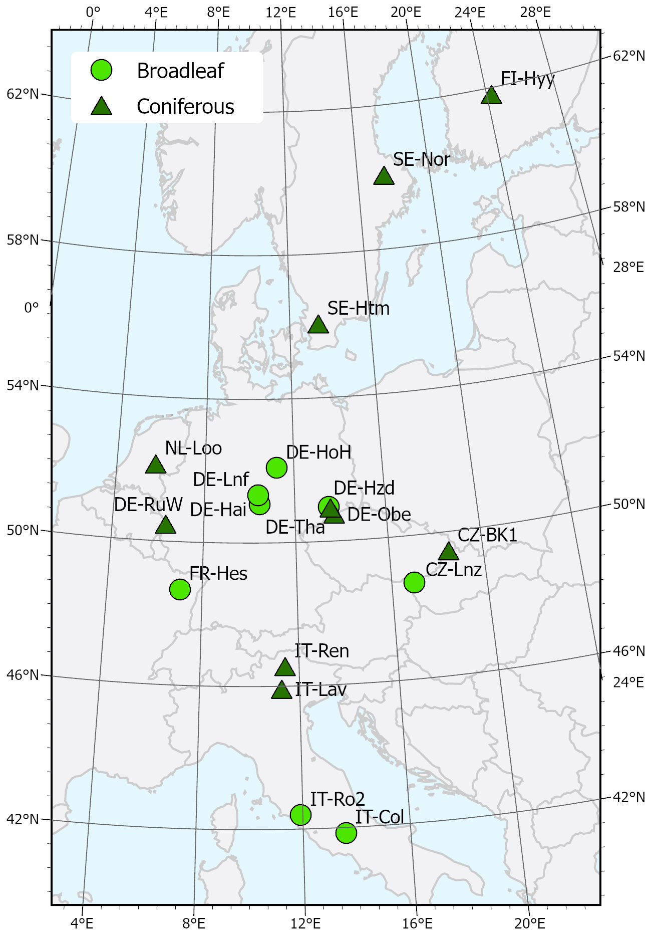
Figure 1 Map of the study sites. Basemap from EuroGeographics.

2.2 Satellite data

The MODIS satellite variables used are listed in Table 1 and are divided into four categories based on the main variable the VIs respond to: surface temperature, vegetation water content, leaf pigments and canopy structure. For simplicity, we refer to all satellite-derived variables (LST, FPAR, LAI and all VIs) as “VIs” even though LST, LAI and FPAR are not VIs in a strict sense. We opted to use MODIS instead of Sentinel-2 due to its much longer archive that allowed us to analyse more different drought periods and ensure that enough sites had drought, reference and post-drought periods that met our criteria. In addition, Cai et al. (2021) showed that forest GPP models were similarly accurate when based on MODIS or Sentinel-2 data.

We used quality-filtered and gapfilled LST data from the FluxnetEO database (v2) representing the area within 1 km of the flux tower (Aqua daytime overpass “average_cutout” dataset; Walther et al., 2022). Similar to the other VIs, we opted to use this product because it provided LST at nadir. We smoothed the LST data using a 15 d moving average to remove day-to-day variations and emphasize longer-term changes due to drought.

PPI and all other VIs were calculated using data downloaded from the NASA EarthData Distributed Active Archive Center or Google Earth Engine, respectively. The data were filtered to remove clouds and low quality data points using the provided quality control layers as described in Table 2. We opted to use the MCD43A4 product because it provides reflectances at nadir corrected for changes in viewing angle. We used the MODIS pixel that contained the flux tower although at some sites the flux tower was within a few meters of the pixel edge (see Table A1). The FPAR and LAI data were noisier than the other indices so to remove outliers in the raw data we applied a median absolute deviation (MAD) filter to these time series. All satellite data except LST were gapfilled and smoothed in TIMESAT 4 (Cai, 2025) using splines to create daily resolution time series. We used the following settings in TIMESAT for all bands: spline smoothing factor = 5000, number of envelope iterations = 1, adaptation factor = 0.

To check if the time series contained significant trends over time (e.g. due to forest growth increasing the seasonal amplitude of a VI over time), we fit linear regressions to the annual 90th percentile value of each VI for each site. If the slope of the regression was significantly different from 0, the time series was detrended.

2.3 Eddy covariance data

We used data in the FLUXNET Archive format from the FLUXNET database, the ICOS ETC L2 Archive and ICOS Warm Winter 2020 products which all follow comparable data processing chains (see Table 3, Pastorello, et al., 2020). The daily nighttime partitioned GPP (GPP_NT_VUT_REF) was used and filtered to exclude days which contained less than 50 % measured or good quality gapfill data according to NEE_VUT_REF_QC (i.e. the quality control flag for the net ecosystem exchange from which GPP_NT_VUT_REF is modelled). After a visual check of the GPP we removed data during periods where gapfilling had failed and produced multiple consecutive weeks with a single constant GPP or respiration value or near-identical weekly oscillations. We also used a MAD filter to remove outliers. To remove long-term trends in GPP we fit standard linear regressions to all data (daily resolution) in each time series. If the slope of the regression was significantly different from 0 (based on a Wald test), the GPP was detrended. The daily GPP timeseries was then smoothed using a 15 d moving average to remove high frequency noise and emphasize longer-term changes due to drought.

2.4 Drought index

We used the Standardized Precipitation Evapotranspiration Index (SPEI) to determine meteorological drought periods (Vicente-Serrano et al., 2010). The SPEI was calculated for each flux site from 1981–2022 at 0.1° spatial resolution and quasi-weekly temporal resolution (day 1, 9, 16, and 23 of each month), using the Multi-Source Weighted-Ensemble Precipitation dataset (Wang et al., 2026) and the University of Bristol's potential evapotranspiration dataset (Singer et al., 2020). A 3-month aggregation was chosen because vegetation responds most strongly to drought at shorter aggregations of the SPEI (Vicente-Serrano et al., 2013). The pseudo-weekly SPEI was linearly interpolated to a daily timestep to enable higher temporal resolution of drought start and end dates.

2.5 Z-score calculation

Z-scores for each VI and GPP time series were calculated by subtracting the mean of each day of year (DOY) across all years, then dividing by the standard deviation of each DOY across all years. The mean and standard deviation were calculated using only days when SPEI-3 was between −1.5 to 1.5 to ensure they represented average climate conditions. The yearly time series of DOY mean and standard deviation for each site was smoothed using a 30 d moving average prior to z-score calculation to ensure it represented a smooth seasonal cycle. Any GPP or VI z-score values $<-\mathrm{6}$ or >6 were discarded as outliers. The z-scores of GPP and the VIs were used in all further analysis.

Within each site, the z-scores of some VIs were highly correlated to each other, producing near identical times series (Fig. A1). EVI, EVI2 and NIRv as well as NMDI and NDWI all had correlations >0.8, therefore we excluded EVI, EVI2 and NMDI from any further analysis, keeping only NIRv and NDWI.

2.6 Selection of drought periods

We identified periods when meteorological drought occurred and had a negative impact on GPP based on the following criteria:

1. SPEI-3 < −1.5 for at least 21 consecutive days during the growing season

2. GPP z-score < −1 for at least 10 consecutive days during the drought

3. GPP data is available during ≥75 % of the drought period

The growing season was defined as the period when GPP exceeded 10 % of the yearly maximum GPP. Droughts in consecutive years were excluded. This produced a sample size of 31 droughts, 17 droughts from 10 coniferous sites and 14 droughts from 8 broadleaf sites (see Table 3) that were used in the following analyses. Some sites experienced multiple droughts. We used a different threshold for GPP compared to SPEI to define drought to ensure a large enough sample size remained for the analysis. We chose to focus on drought periods that have a noticeable negative impact on GPP as suggested by Reichstein et al. (2013) and use a similar definition as previous studies such as Yu et al. (2022). This was also important to help narrow the focus of this study since drought can also cause no impact or even a positive impact on GPP which would lead to different responses in the VIs. Focusing only on periods when GPP was negatively affected allowed us to examine the time lags between GPP and VI response to drought and thus help identify why some VIs weren't able to capture GPP declines due to drought.

Table 1 MODIS satellite variables used in the analysis. Note that due to the high correlation between some of the VI z-scores (Fig. A1, Sect. 2.5) only the results from LST, NDWI, CCI, PRI10, NDVI, LAI, FPAR, PPI and NIRv are presented here. Footnotes provide the dataset citations. n/a = not applicable.

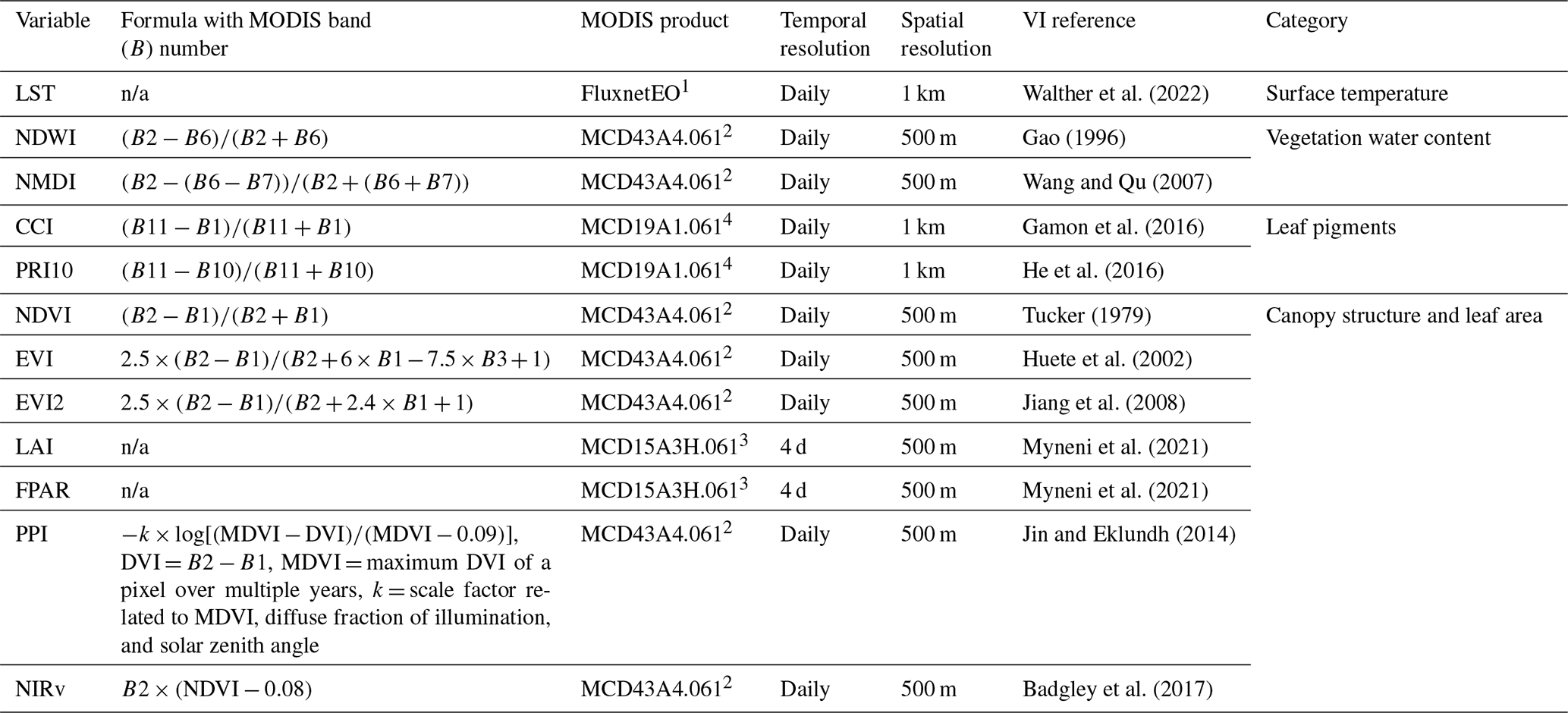
¹Walther et al. (2023). ²Schaaf and Wang (2021). ³Myneni et al. (2021). ⁴Lyapustin and Wang (2022).

Table 2 Quality filtering information for each satellite variable.

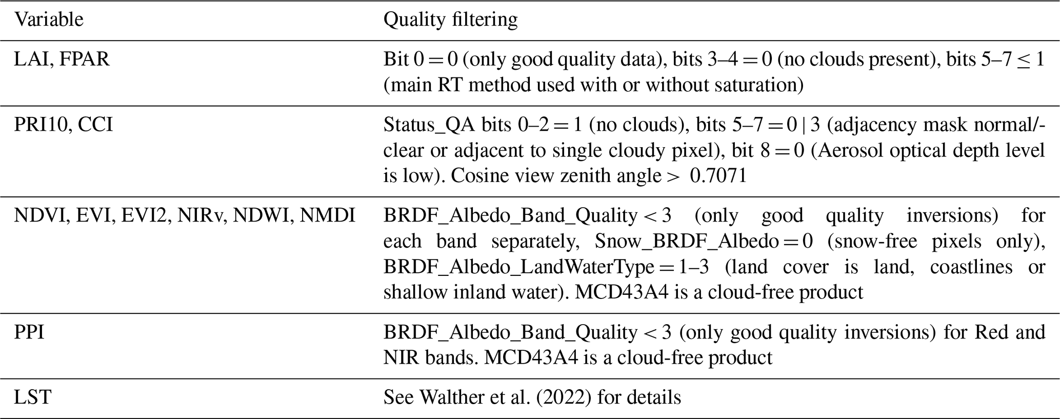
Table 3 Sites used in the analysis including drought period as defined by SPEI-3. Mean annual temperature (MAT) and mean annual precipitation (MAP) are calculated using ERA5-Land data for the climate normal period 1991–2020. LAI is from in-situ measurements from ICOS ETC L2 Archive ancillary data files (averages of LAI measured between June–August across all available years) or from literature describing the site. n/a = not applicable.

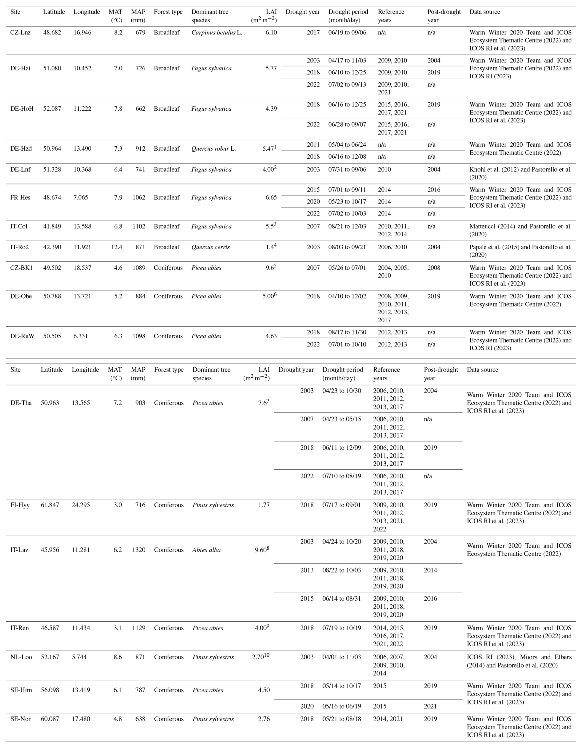
¹Bernhofer et al. (2025). ²Anthoni et al. (2004). ³Scartazza et al. (2013). ⁴Rey et al. (2002). ⁵Sedlák et al. (2010). ⁶Zimmermann et al. (2006). ⁷Grünwald and Bernhofer (2007). ⁸Marcolla et al. (2003). ⁹Montagnani et al. (2025). ¹⁰van der Molen et al. (2025).

2.7 Analysis of drought response time lags

We identified the dates for drought response start (Date_start), maximum drought impact (i.e. GPP or VI minimum, Date_min) and end of drought response (Date_end) separately for GPP and each VI z-score for each drought event. The criteria used to define these three dates are listed in Table 4.

Table 4 Criteria used to define Date_start, Date_min and Date_end for z-scores of GPP and each VI.

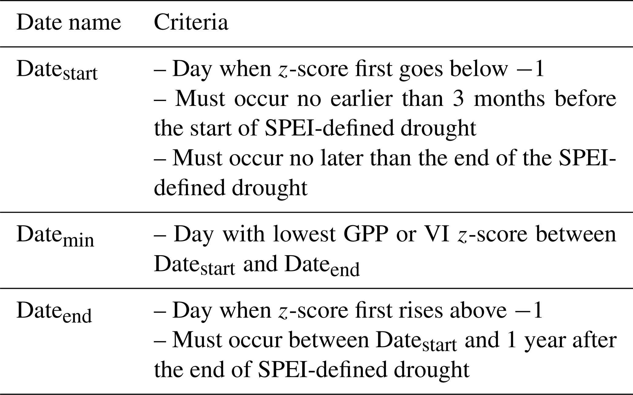
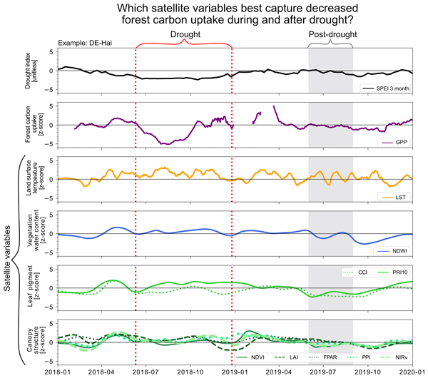
Examples of the Date_start, Date_min and Date_end are provided in Fig. 2. We note that since LST is expected to increase during drought, the criteria were inverted: LST Date_start corresponds to the date when LST z-score > 1, LST Date_min is the date of maximum LST z-score and LST Date_end is the date when LST z-score becomes <1.

We did not find a Date_start for all VIs in all droughts (i.e. some VI z-scores never dropped below −1 during the search period, see example in Fig. 2a) and therefore we did not identify Date_min or Date_off for these cases. Out of a total of 31 droughts, there were only 2 droughts for which we could identify Date_start, Date_min and Date_end for every VI and GPP. To be able to use a larger sample size in our analysis, we included all drought periods that a VI responded to (i.e. Date_start existed), even though this led to different subsets of droughts being used for each VI.

To analyse the drought response lag times, we calculated the average number of days between the Date_start, Date_min or Date_end for each VI and GPP. We also compared the VI and GPP response times with SPEI drought start and end dates.

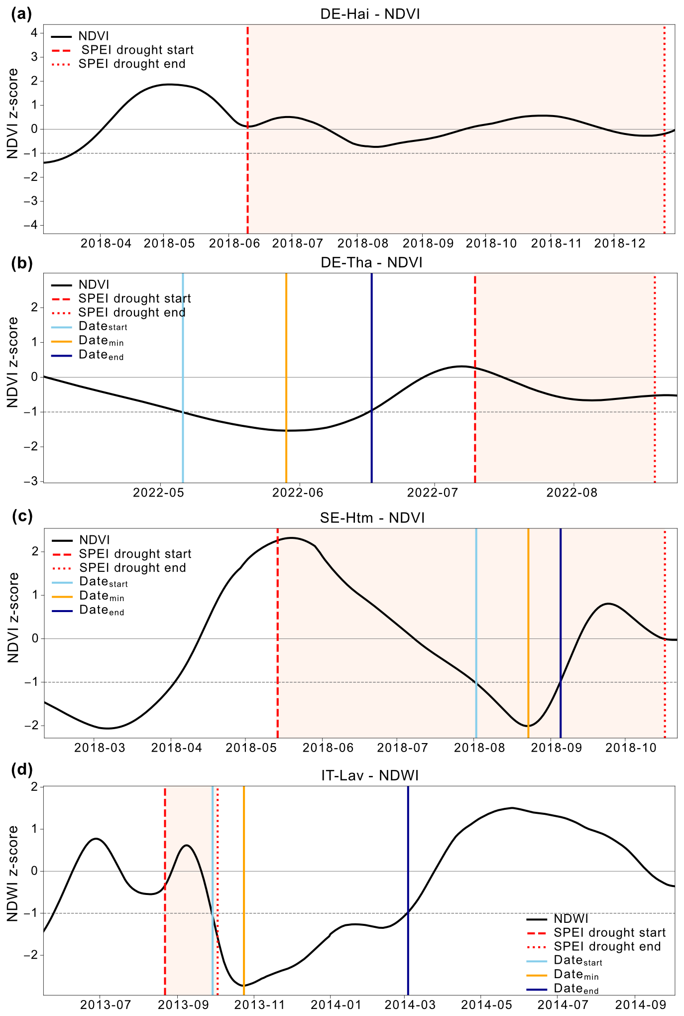
Figure 2 Examples of time lag analysis from different sites and drought periods. (a) No Date_start, Date_min or Date_end identified. (b) NDVI drought response period preceding SPEI drought period. (c) NDVI drought response period overlapping with SPEI drought period. (d) NDWI drought response period occurring mostly after SPEI drought period.

2.8 Comparison of VIs and GPP between drought and reference periods

To determine whether each VI responds to drought, we tested for significant differences in each VI between drought and non-drought reference periods. To do this, we used the droughts identified previously (see Table 3) for which at least one valid reference period existed. A reference period was defined using the following criteria:

1. Period starting and ending on the same date as the drought (based on SPEI) in a year when no drought occurred

2. GPP data was available for ≥75 % of the reference period

3. Cannot occur within two years after a drought

4. Mean GPP z-score during reference period must be greater than mean GPP z-score during drought period

After these filtering steps, there were 28 drought and reference periods at 10 coniferous sites and 6 broadleaf sites, with the sites covering a wide latitudinal gradient (see Table 3).

We calculated the average GPP and VI z-score during each drought and reference period, using the GPP drought response dates (i.e. between GPP Date_start and Date_end, but changing the year for the reference period). This average GPP or VI z-score per site and drought or reference period was used as the dependent variable in a linear mixed effects model (separate models were fit to each VI and GPP), using the following model form:

$$\begin{array}{}\text{(1)}& \begin{array}{rl}{Y}_{ij}& ={\mathit{\alpha }}_j+{\mathit{\beta }}_{\mathrm{1}}{\mathrm{stage}}_{ij}+{\mathit{\beta }}_{\mathrm{2}}{\mathrm{foresttype}}_{ij}\\ & +{\mathit{\beta }}_{\mathrm{3}}\left({\mathrm{stage}}_{ij}\times {\mathrm{foresttype}}_{ij}\right)+{\mathit{ϵ}}_{ij}\end{array}\end{array}$$

Where Y_ij is the mean z-score of GPP or a VI during a drought or reference period for observation i in site j, the fixed effects are stage (categorical variable for reference or drought period), foresttype (categorical variable for coniferous or broadleaf forest) and their interaction and ϵis the residual error. α_j denotes the random effect (intercept) of site, which accounts for the multiple drought periods per site. Models were fit using the nlme R package (Pinheiro et al., 2023). If needed, a variance structure (varIdent, described in Zuur et al., 2009) with stage and/or forest type as covariate was included to account for large differences in model residual variance between stages and/or forest types. In some cases, the random effects could not be determined and the model was refit without random effects using the gls (generalized least squares) function.

To determine whether there was a significant effect of stage, forest type or their interaction on GPP or each VI, ANOVAs followed by post-hoc pairwise Tukey tests (emmeans package, Lenth and Piaskowski, 2025) were conducted. Marginal R² ($R_{\mathrm{marg}}^{\mathrm{2}}$, the variance explained by the fixed effects only) and conditional R² ($R_{\mathrm{con}}^{\mathrm{2}}$, variance explained by the fixed and random effects) were used to describe model performance. $R_{\mathrm{marg}}^{\mathrm{2}}$ and $R_{\mathrm{con}}^{\mathrm{2}}$ were calculated using the performance package (Lüdecke et al., 2021) based on (Nakagawa and Schielzeth, 2013).

We also assessed whether there was an effect of drought severity on mean VI z-score during drought by calculating spearman's rank correlation coefficients for each VI versus minimum SPEI during drought (using drought dates based on GPP Date_start and Date_end). Correlations were calculated separately for broadleaf and coniferous sites, using the same drought periods as included in the mixed effects modelling analysis.

2.9 Assessing post-drought effects in GPP and VIs

We used a smaller subsample of drought events that had both a valid reference and post-drought year to investigate whether post-drought effects were visible in GPP and/or the VIs. A post-drought year was defined as the first year after a drought (with no drought occurring during that year). We only used sites where the drought period overlapped with the peak growing (June to August) season to ensure similar types of droughts and post-drought effects during the same time of year were compared between sites. There were 13 valid reference, drought and post-drought groups at the coniferous and 6 at the broadleaf sites, respectively (see Table 3). We tested whether there was a significant difference in mean GPP or VI z-score during the peak growing season between reference and post-drought years using a paired t-test or a Wilcoxon signed rank test if the data were not normally distributed. We used the Benjamini-Hochberg method to adjust the p-values for multiple testing (Benjamini and Hochberg, 1995). If multiple reference years were available we used the average over all reference years. We were not able to use mixed effects analysis due to the small sample size.

3 Results

3.1 Drought response lag times

We compared the timing of Date_start, Date_min and Date_end between GPP and each VI (Fig. 3a to f). For both forest types there were overlaps in drought response timing (seen as large standard deviations in Fig. 3a to f) among all the VIs and between the VIs and GPP. Nevertheless, there were differences in the response timing between broadleaf and coniferous sites. At the broadleaf sites, there was a more distinct pattern: NDWI and LST responded before GPP, followed by the leaf pigment indices and finally the canopy structure indices responded last, often after GPP (Fig. 3a, c and e). At the coniferous sites, the difference in timing of Date_start between GPP and the VIs was low, but for most VIs, Date_min and Date_end occurred over a month earlier than GPP (although with standard deviations ranging between 26 to 92 d; Fig. 3d and f).

It is important to note that not all VIs responded to drought (i.e. where no Date_start was identified, Fig. 3g and e). In particular, LAI and FPAR responded only to a third of droughts or less across all broadleaf and coniferous sites. LST on the other hand responded to every drought in both forest types. At the broadleaf sites, CCI had the second highest drought response rate (93 %) whereas at the coniferous sites it was PPI (71 %).

Figure 4a shows that GPP started responding negatively to drought (Date_start) at the same time as the SPEI drought start date at broadleaf sites. Most of the structure-related VIs, however, started responding to drought almost two months after the SPEI drought start date. At the coniferous sites (Fig. 4b), GPP response lagged the SPEI drought start date by 14 d on average and all the VIs except LST showed lagged responses to drought start compared to SPEI. The date of the most severe drought impact (Date_min) on GPP was very close to the date of the SPEI minimum for both forest types (Fig. 4c, d). In terms of drought end date, however, all the VIs and GPP stopped responding (Date_end reached) to drought before drought ended according to SPEI (Fig. 4e, f). Indeed, drought was longest when measured using SPEI compared to any of the VIs or GPP (based on time between Date_start and Date_end, Fig. 4g, h).

We note that the difference (in number of days) between a VI and GPP Date_start (or Date_min or Date_end) will be different in Fig. 4 compared to Fig. 3. This is because GPP responds to all drought periods (as per the study design) whereas all the other VIs except LST responded to a smaller number of droughts (Fig. 3g and h). Therefore, the average time differences shown for GPP in Fig. 4 are calculated for a larger sample size than was used when comparing responses between GPP and each VI in Fig. 3. Hence the difference in the timing between a VI and GPP should not be compared between Figs. 3 and 4.

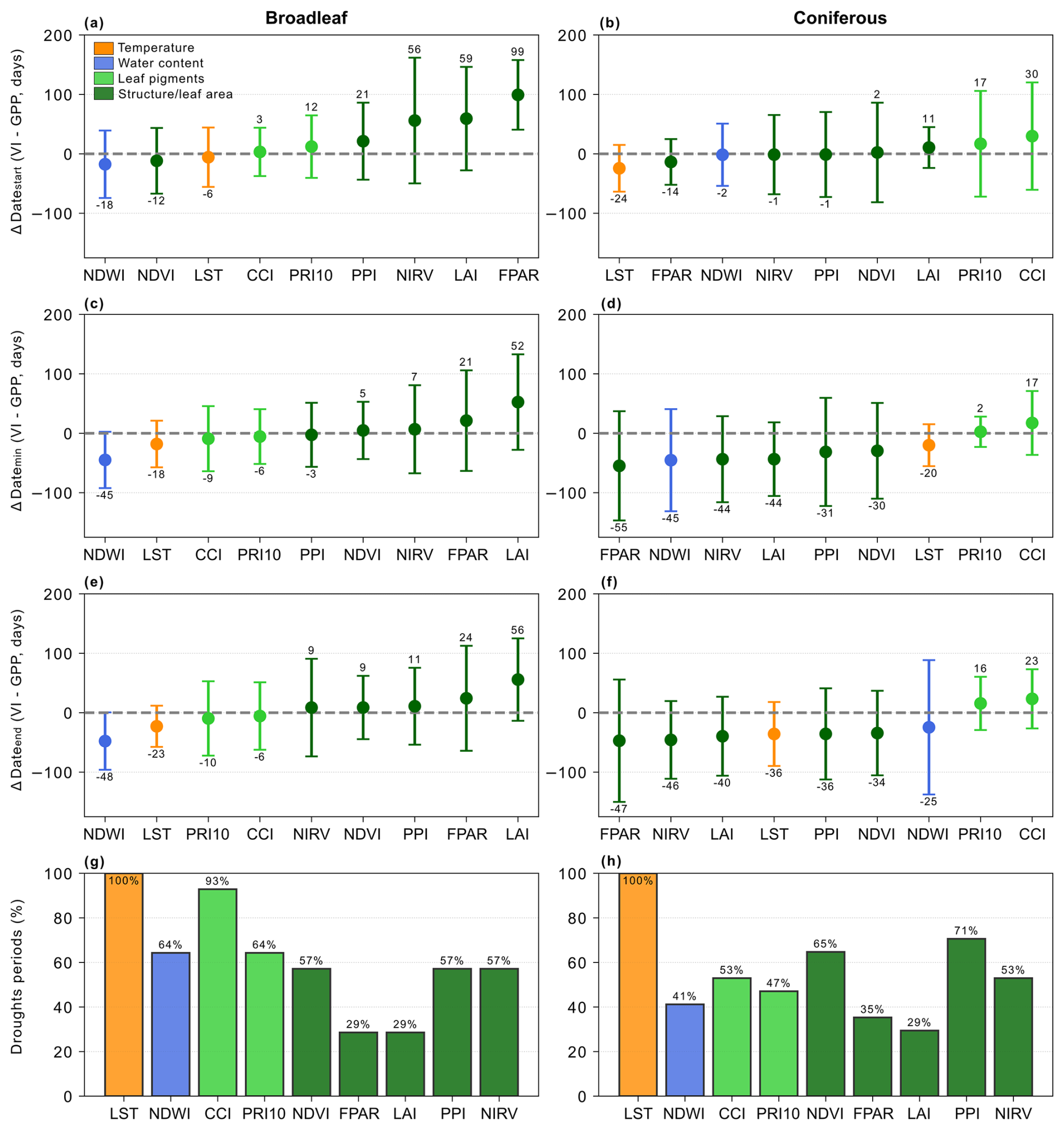
Figure 3 Mean ± standard deviation of difference between (a, b) Date_start, (c, d) Date_min and (e, f) Date_end of VIs and GPP at broadleaf (left) and coniferous (right) sites. Negative number means the VI date preceded the GPP date. Numbers above or below the error bars are the mean difference in days. (g, h) show the percentage of droughts where Date_start was found for each VI (i.e. VI responded to that drought). Bar colour refers to the VI category (orange = land surface temperature, blue = vegetation water content, light green = leaf pigments, dark green = canopy structure/leaf area). Note that VI order changes in each plot.

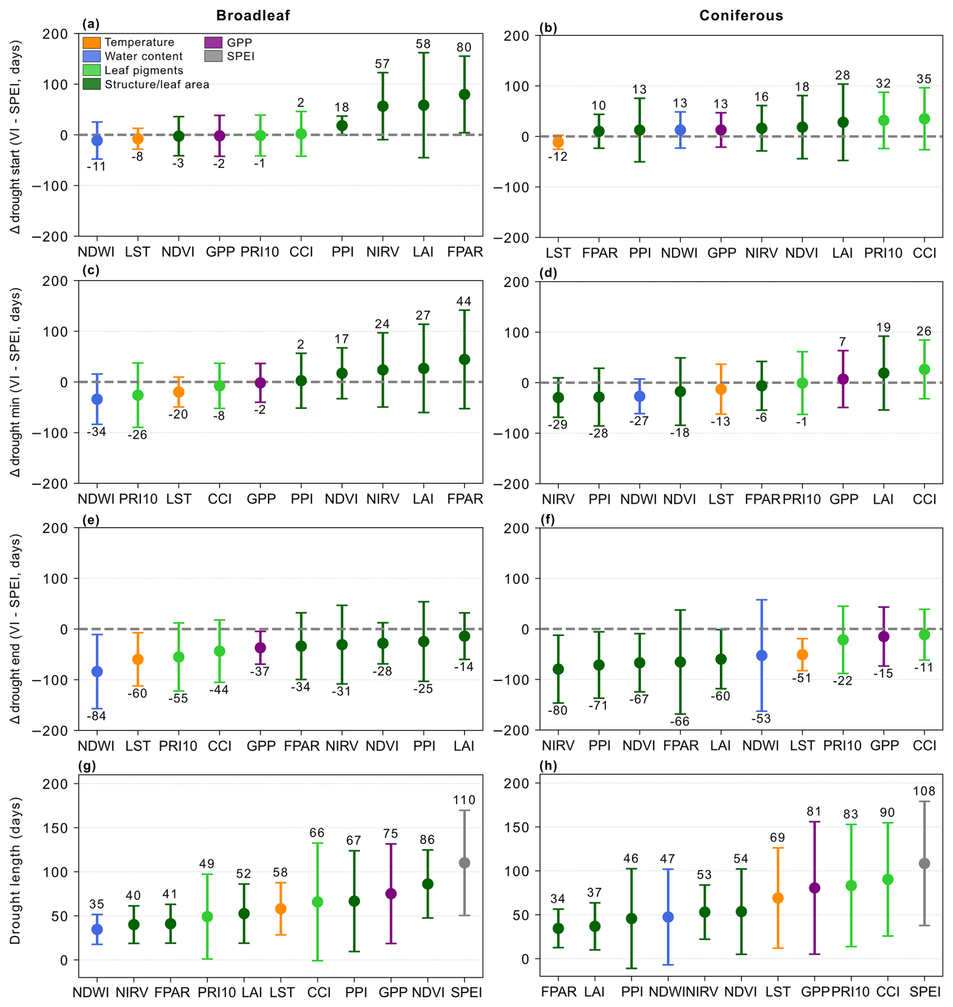
Figure 4 Mean ± standard deviation of difference between VI or GPP drought start, minimum and end dates and SPEI: (a, b) VI or GPP Date_start minus SPEI drought start date (c, d) VI or GPP Date_min minus date of SPEI minimum value during drought (e, f) VI or GPP Date_end minus the SPEI drought end date (g, h) drought length for each VI and GPP (between Date_start and Date_end) and SPEI. Left and right subplots are broadleaf and coniferous sites, respectively. Negative number means the VI or GPP date preceded the SPEI date. Numbers above or below the error bars are the mean. Bar colour refers to the VI category (orange = land surface temperature, blue = vegetation water content, light green = leaf pigments, dark green = canopy structure/leaf area, purple = GPP, grey = SPEI). Note that VI order changes in each plot.

3.2 Comparison of VIs and GPP between drought and reference periods

Mean GPP z-score declined significantly during drought compared to reference periods at both broadleaf and coniferous sites (Fig. 5a). The interaction effect between stage and forest type was also significant because GPP z-score declined more at broadleaf than coniferous sites during drought. Of all the VIs we tested (Fig. 5b–j), only LST changed significantly at both broadleaf and coniferous sites during drought. NDWI, CCI and NDVI were significantly lower during drought than reference periods but only at broadleaf sites (Fig. 5c, d, h), while NIRv was significantly lower but only at coniferous sites (Fig. 5j). FPAR and LAI increased marginally during drought compared to reference periods at both broadleaf and coniferous sites (Fig. 5f, g).

We tried including the random effect of site in all models (see Table 5), but for the NDWI and CCI models it was not possible: the random effect could not be estimated because it explained very little variance. In contrast, for the PRI10, NDVI and NIRv models, including the random effect led to much higher $R_{\mathrm{con}}^{\mathrm{2}}$ than $R_{\mathrm{marg}}^{\mathrm{2}}$, indicating that there were large differences in PRI10, NDVI and NIRv between sites (Table 5).

There were also clear differences in the drought response of different tree genera within each forest type (Fig. 6). It is worth noting that both the broadleaf and coniferous sites experienced similarly severe droughts. Minimum SPEI during drought (based on the GPP response period between GPP Date_start and Date_end) was on average (± standard deviation) −2.1 ± 0.2 and −2.0 ± 0.3 and the average SPEI during drought (same time period) was −1.8 ± 0.2 and −1.6 ±  0.5 at the broadleaf and coniferous sites, respectively. Correlations between mean VI z-score during drought and drought severity (minimum SPEI) were weak for most VIs except LST at coniferous sites (spearman's correlation coefficient = −0.3) and CCI, LAI and NIRv at broadleaf sites (0.47, 0.38 and 0.45, respectively; Fig. A2). We did not observe any thresholds in VI behaviour in response to drought severity (Fig. A2). The GPP drought response lasted longer on average at the coniferous sites (83 ± 75 d) than at the broadleaf sites (68 ± 35 d).

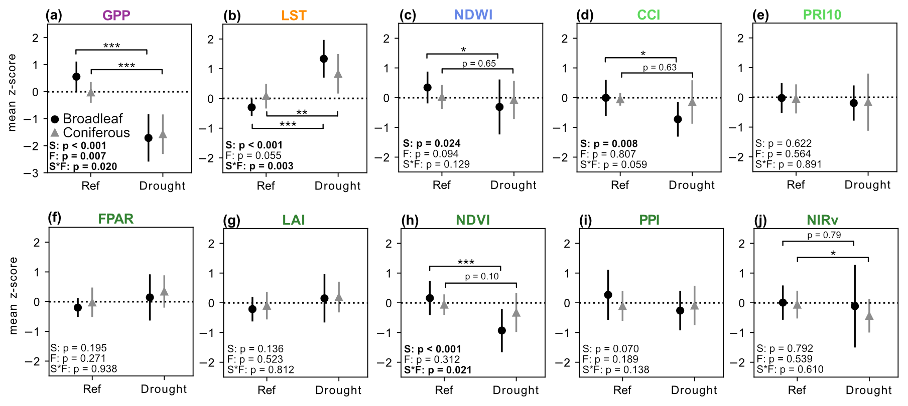
Figure 5 Mean ± standard deviation of mean GPP and VI z-score during reference and drought years using drought response dates defined by GPP Date_start and Date_end. Data from coniferous sites (grey triangle) and broadleaf sites (black circle). P-values from ANOVAs for the main effects of drought stage (S), forest type (F) and stage × type are provided in each subplot, in bold if p<0.05. P-values for the results of pairwise post-hoc Tukey comparisons between reference and drought period for each forest type are plotted only if one of the forest types had a significant result (* = p<0.05, ** = p<0.01, *** = p<0.001). Sample size: 11 drought and reference periods at 6 broadleaf sites and 17 drought and reference periods at 10 coniferous sites.

Table 5 Mixed effect model goodness-of-fit statistics, using all sites. “n/a” means that random effects could not be estimated, the model was fit without random effects. $R_{\mathrm{marg}}^{\mathrm{2}}$ is the marginal R₂ (variance explained by the fixed effects only) and $R_{\mathrm{con}}^{\mathrm{2}}$ is the conditional R² (variance explained by the fixed and random effects).

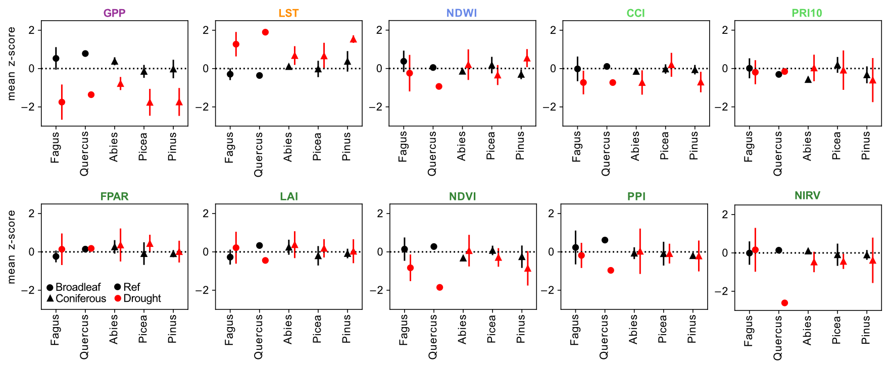
Figure 6 Mean ± standard deviation of mean GPP and VI z-score per dominant site tree genera during reference (black) and drought years (red) using drought response dates defined by GPP Date_start and Date_end. Data from coniferous sites (triangle) and broadleaf sites (circle). Quercus does not have a standard deviation because there was only one drought and reference period for that genus.

3.3 Post-drought effects in GPP and VIs

We found no significant differences in mean z-score between reference and post-drought periods for GPP or any of the VIs (Fig. 7). Nevertheless, for NDWI, PRI10, NDVI, PPI and NIRv (Fig. 7c, e, h, i, j), the mean z-score during the post-drought period was lower than during the drought and the reference periods. For these VIs, broadleaf sites tended to have lower post-drought mean z-scores than coniferous sites. In contrast for GPP, LST, CCI, FPAR and LAI (Fig. 7a, b, d, f, g), the post-drought mean z-scores were close to 0 and similar to the reference mean z-scores. It is worth noting that broadleaf GPP did not completely recover in the post-drought year but remained lower than the reference year GPP z-score.

Examples of the different post-drought response between GPP and the VIs are shown for DE-Hai (Fig. A3), DE-Lnf (Fig. A4) and SE-Htm (Fig. A5) for different drought events. At DE-Hai, GPP recovered close to 0 in the post-drought year, yet NDWI, NIRv, NDVI and PPI reached lower minimum values during the peak-growing season of the post-drought compared to the drought year. The same pattern was also visible at DE-Lnf, although GPP was also relatively low in the peak-growing season of the post-drought year (fluctuating around −1). At SE-Htm, post-drought GPP was higher than average (z-score > 0) yet the NDWI, CCI and the structural VIs were lower on average than in the drought year.

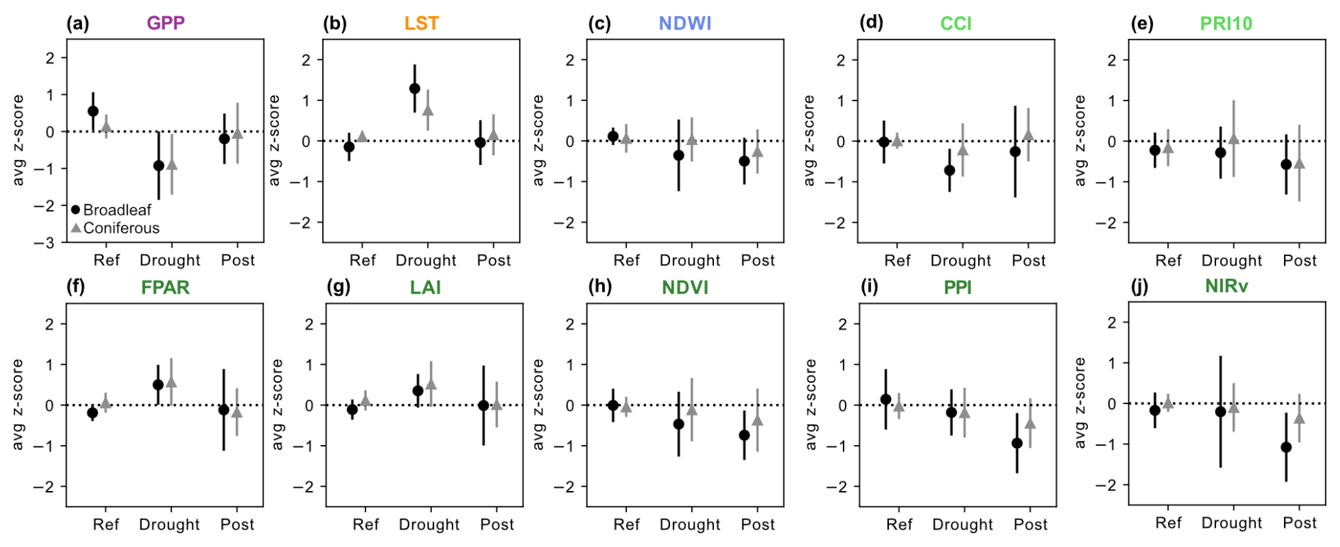
Figure 7 Mean ± standard deviation of mean z-score during peak growing season (June–August) of reference, drought and post-drought years for GPP and each VI at coniferous sites (grey triangle) and broadleaf sites (black circle). None of the pairwise t-tests or Wilcoxon signed rank tests between reference and post-drought mean z-score were significant. Pairwise tests were not performed using the drought z-scores but they are plotted for comparison.

4 Discussion

4.1 Drought response timing

Our analysis of the timing of drought response confirmed that using SPEI with a three month aggregation time was appropriate for identifying the period when GPP negatively responds to drought in European forests. This was partly due to the way drought was defined (based on both SPEI and GPP) but still highlights the close alignment of GPP with SPEI-3. In fact, at broadleaf sites, GPP stopped responding to drought on average more than a month before the drought finished as defined by SPEI, which suggests an even shorter SPEI aggregation period may work better for these sites. However, using a shorter aggregation period introduces more high-frequency variation into SPEI which may lead to difficulties identifying sustained and severe drought periods. Similarly, Jin et al. (2023) and (Vicente-Serrano et al., 2013) found that short SPEI timescales (<5 months) showed the highest correlation between SPEI and multiple VIs across Europe and globally. Using longer SPEI aggregations, which cause drought start and end dates to occur later than shorter SPEI aggregations, would therefore not be appropriate for capturing drought impacts on European forest GPP.

Despite exposure to droughts of similar severities, we found different patterns in the timing of drought response for VIs at broadleaf compared to coniferous sites, although there were large overlaps in the response timing among the VIs. Tree drought responses are sensitive to local site conditions and drought characteristics (Rita et al., 2020; Sturm et al., 2022). The large variability (i.e. large error bars in Fig. 3) in drought response timing for each VI as well as the mostly weak relationships between VIs and drought severity (Fig. A2) we observed were likely driven by the highly variable sites and drought conditions we compared (e.g. differences in site topography, aridity, mean annual temperature and precipitation, soil type, soil water storage, tree species, tree age as well as drought length, severity and timing).

Broadleaf sites tended to experience an immediate reduction in canopy water content (likely linked to falling leaf water potentials) and increased canopy surface temperature (likely linked to declining canopy conductance, reduced transpiration, and increased radiative heating) that started on average 1 to 3 weeks before GPP Date_start (Fig. 3a). These results are supported by plant physiology experiments showing that stomatal closure is the first drought response of C₃ plants that limits photosynthesis in the early phase of drought (Flexas and Medrano, 2002). Reductions in leaf chlorophyll to carotenoid ratios, which indicate the downregulation of photosynthesis due to stress, then occurred within 3 to 12 d after GPP Date_start (Fig. 3a). Several studies have shown that leaf shedding lags the start of drought (West et al., 2022; Zhang et al., 2016), and our study confirmed that this effect was visible between 2 weeks to almost 3 months after the drought start according to SPEI (for PPI, NIRv, LAI and FPAR) depending on the VI used (Fig. 3a). Interestingly, NDVI responded much earlier than the other structural VIs (discussed more below).

The lack of a pattern in VI drought response at the coniferous sites was likely due to the weaker response of VIs to drought at these sites (Fig. 3b). In addition, the coniferous sites spanned a much larger latitudinal range than the broadleaf sites, leading to higher between-site variability in drought response.

4.2 Surface temperature and canopy water content response to drought

We found that LST was the VI that had the strongest and most consistent response to drought of all the VIs we tested (Figs. 3g–h and 6). In addition, LST did not exhibit any post-drought legacy effects, similar to GPP, indicating that it could reliably capture the period when GPP is affected by drought (Fig. 7). Although the superior performance of LST over the VIs may partly be due to the additional quality filtering, nadir correction and gapfilling that was included in the FluxnetEO product, it is unlikely to be the main reason. We also note that the high response rate of LST to SPEI-defined drought is not unexpected as SPEI is calculated using temperature and solar radiation variables that likely co-vary with LST. Nevertheless, severe drought leads to high radiative heating of the upper tree canopy along with reductions in canopy conductance and hence reduced transpiration that results in higher leaf temperature then visible in LST images (Scherrer et al., 2011). Our results are supported by Hoek van Dijke et al. (2023) who found that LST increase during drought matched the timing of stomatal conductance decline due to drought at forest sites better than NDVI, EVI or NIRv. We showed that this response can be detected at both coniferous and broadleaf sites and was present during every drought period we tested. Our results therefore suggest that remote-sensing based models of GPP should use LST as an input to capture drought-related GPP decline in forests. In fact, site-level studies using thermal imagery in forests have found that GPP or NEE is more closely related to canopy surface temperature than to air temperature (Pau et al., 2018; Kim et al., 2016). Similarly, Montero et al. (2024) found that including LST in machine learning models improved GPP prediction during climate extremes, including drought.

We found that LST increased more during drought at broadleaf than coniferous sites, which could be explained by results from a site-level thermal camera study in a temperate forest in Switzerland (Leuzinger and Körner, 2007). The study showed that areas dominated by dense canopies of broadleaved species such as Fagus sylvatica (which is the dominant species at our broadleaf sites) had higher canopy temperatures than areas dominated by coniferous species. They attributed the differences to a combination of characteristics such as leaf density, width and canopy roughness that resulted in dense broadleaf canopies being less coupled to the atmosphere (higher leaf boundary resistance) than coniferous canopies.

NDWI was also more sensitive to drought at the broadleaf than the coniferous sites, but this may simply reflect species-specific drought survival strategies within each forest type (Figs. 5 and 6). For example, isohydric genera like Pinus close stomata earlier than anisohydric genera like Fagus when experiencing water stress and thus are able to maintain stable midday leaf water potentials (D'Odorico et al., 2025). This may explain how Pinus maintained such high NDWI values during drought but also had very high LST (since transpiration would have been reduced). In addition, coniferous species tend to lose less water when stomata are closed than broadleaf species (Wang et al., 2024). These factors may help keep leaves hydrated and maintain turgor pressure for longer during drought meaning that NDWI changes less for coniferous compared to broadleaf species during drought. Finally, NDWI is also sensitive to changes in leaf area, since changes in leaf area lead to changes in total water content within a NDWI pixel (Zarco-Tejada et al., 2003). Since broadleaf genera appeared to exhibit higher rates of leaf discoloration and wilting during drought than coniferous species (seen in their lower NDVI values, Figs. 5 and 6), this change would also be reflected in the NDWI data for the broadleaf sites. At our sites, NDWI z-scores had a correlation of 0.48 to NDVI z-scores, confirming the shared information between these two indices.

It is worth noting that some studies of the 2018 drought (e.g Wang et al., 2025) found that conifer dominated areas suffered more from drought than broadleaf dominated areas, including Sturm et al. (2022) who used NDWI to track drought impacts in Swiss forests. But the divergence between our findings and these studies can be explained at least partly by the species being studied. For example, Picea abies is one of the most dominant coniferous species in Switzerland and is known to be very vulnerable to drought. We also found that NDWI declined for Picea abies during drought but not for the other coniferous genera (Fig. 6). It is thus important to keep in mind that genera-specific changes drive the overall response of the coniferous and broadleaf categories for each of our VIs.

4.3 Leaf pigment response to drought

Our results confirm that CCI is well-suited to capturing drought-impacts on broadleaf GPP and performs better than PRI10 which was calculated in the same way but using a band 10 instead of band 1 as a reference band. These findings are supported by site-level studies showing that Fagus sylvatica relied more heavily on the xanthophyll cycle during drought compared to coniferous species (D'Odorico et al., 2025) and showed strong increases in measured leaf carotenoid content and decline in chlorophyll content during drought (Nestola et al., 2018) which are significant enough to be captured by coarse-scale MODIS data as shown here. At the coniferous sites, average CCI appears not to change during drought, which is surprising since CCI is known to closely track GPP phenology at coniferous sites (Gamon et al., 2016). But this must be due to the genera-specific behaviour of CCI at the coniferous sites: all coniferous genera at our sites except Picea abies showed noticeable declines in average CCI during drought (Fig. 6). Since the Picea abies sites experienced equal or more severe declines in GPP during drought compared to the other coniferous sites, differences in CCI behaviour cannot be attributed to differences in drought severity. Further research is needed to understand the differences in behaviour between coniferous genera spectral response to drought.

4.4 Canopy structure and leaf area response to drought

The canopy structure and leaf area VIs can be split into two groups based on their responses to drought. The first group is FPAR and LAI, which both increased (but not significantly) during drought at broadleaf and coniferous sites (Fig. 5). We believe that the ability of these two indices to capture drought-related declines in greenness and leaf area was low due to the fact that (i) their raw time series were much noisier than any of the other VIs we tested and (ii) they are modelled variables. Even under non-drought conditions, Jin and Eklundh (2014) showed that MODIS LAI had a much lower correlation to field measured LAI than NDVI, EVI or NDVI. Our results suggest that MODIS LAI and FPAR should not be used alone as indicators of drought-related GPP reductions in forests and must be combined with other VIs or meteorological constraints.

In the second group are NDVI, PPI and NIRv, that either declined or did not respond to drought (Fig. 5). NDVI stood out because it was the only VI that declined during drought at both broadleaf and coniferous sites, and the timing of NDVI decline closely matched that of GPP (Fig. 3a, b). If we start by comparing NDVI with PPI, NDVI is known to correlate with leaf chlorophyll content (Tucker, 1979) whereas PPI was specifically designed to be linearly related to green leaf area (Jin and Eklundh, 2014). At a Fagus sylvatica forest, Nestola et al. (2018) found no relationship between DVI (that PPI is based on) and measurements of leaf chlorophyll content, but a strong relationship between NDVI and chlorophyll content. Since the degradation of leaf chlorophyll precedes leaf shedding (Munné-Bosch and Alegre, 2004), NDVI should start responding before PPI and therefore closer in time to GPP. This assumption has some support from our time lag analysis that showed that NDVI Date_start occurred on average a month earlier than PPI Date_start at the broadleaf sites, although there were large overlaps in the error bars between the two indices.

Interestingly, NIRv showed a noisier (larger error bars) and more delayed response to drought than NDVI (Fig. 3a). This at least partly explained why NIRv did not show a significant difference during drought in the mixed modelling analysis since the analysis was based on the GPP response dates (and NIRv started responding to drought much later than GPP at the broadleaf sites). NIRv was designed to minimize the signal from non-vegetated areas in a pixel and the differences between NIRv and NDVI should be especially pronounced in sparsely vegetated areas (Badgley et al., 2017). However, most of our sites had high LAI (Table 3) so this cannot explain the different responses of the two VIs. Another factor could be that NIRv is relatively more confounded by changes in leaf angle distribution than NDVI and leaf angle is likely to have changed during drought (Kattenborn et al., 2024). Drought-related changes in leaf angle are likely to have been larger at the broadleaf than at the coniferous sites which could explain why NIRv decreased significantly during drought at the coniferous but not at the broadleaf sites (Fig. 5j). Nevertheless, the coarse resolution of the MODIS data we used should have lessened the confounding effect of changes in leaf angle distribution (Kattenborn et al., 2024). In any case, our finding of NDVI sensitivity to drought-related changes in forest greenness are confirmed by a multitude of studies (Brun et al., 2020; Wang et al., 2025; Schuldt et al., 2020).

4.5 Post-drought legacy effects

We observed that several VIs commonly used to model GPP (NDVI, PPI, NIRv) showed noticeable but not statistically significant post-drought legacy effects that were not reflected in GPP (Fig. 7). These results highlight that decoupling between GPP and VIs may occur post-drought.

How can GPP remain high while leaf area and canopy greenness decrease? Studies of thinning in both coniferous and broadleaf forests have shown that GPP decreases less than expected for the given decrease in LAI because of increased understory vegetation growth (Vesala et al., 2005) and increased access to light within the tree canopy that becomes less dense (Granier et al., 2008). In addition, conifers may shed older, less photosynthetically efficient needles (Seidling, 2007).

There are many studies showing that reductions in leaf area are a lagged response to drought that can occur in the post-drought year, which help explain the reductions in the VIs we observed in the post-drought year. Brun et al. (2020) for example found that trees that experienced early wilting during drought also had reduced NDVI in the following spring. For many tree species, drought leads to fewer leaves and lower leaf surface area within each bud formed which is visible in the following year when the buds open (Bréda et al., 2006). For coniferous species, needles may be shed in the autumn following drought and needles grown post-drought are both fewer in number (due to less budset) and shorter due to depleted carbon reserves within the tree (Seidling, 2007). In beech, drought stress can trigger higher than normal seed production in the following year, meaning less biomass is allocated to leaf production (Bréda et al., 2006).

The depression of greenness VIs can last up to 4 years post-drought (Müller et al., 2024; Wu et al., 2018), which would have serious consequences for our ability to model GPP post-drought if the GPP-VI decoupling we observed is persistent and widespread. More research is needed to understand whether the decoupling between GPP and VIs we have observed lasts longer than the first post-drought year and why it occurs at some sites but not others.

5 Conclusion

Optical remote sensing data have become key tools for modelling carbon exchange in forests and quantifying their resilience to drought. Our study highlighted that LST, CCI and NDVI are the VIs best able to track drought-related GPP declines in forests because the timing of their response most closely matches that of GPP. They also showed significant changes during drought compared to reference periods, at least for broadleaf sites. Other commonly used greenness indices such as PPI and NIRv lagged the start of drought impacts on GPP by up to 2 months at broadleaf sites. Modelling GPP during drought will likely be more accurate for broadleaf than coniferous sites since none of the VIs we tested (except for LST and NIRv) declined significantly during the drought year at coniferous sites, despite significant reductions in GPP. We also found noticeable but not statistically significant drought-legacy effects in all the greenness-related VIs that are commonly used to model GPP (NDVI, PPI and NIRv), that are not reflected in flux tower GPP at all sites. The decoupling between GPP and these VIs could lead to underestimation of GPP and the resilience of the forest carbon sink during the post-drought years at some sites. More research is needed to understand how widespread this decoupling effect is and over how many years it occurs. Future work should also test whether the relative performance of the VIs we tested remain consistent when using alternative MODIS or Sentinel products.

Appendix A

Table A1 Distance (m) of each flux tower from the nearest MODIS pixel edge for 500 m and 1 km resolution bands.

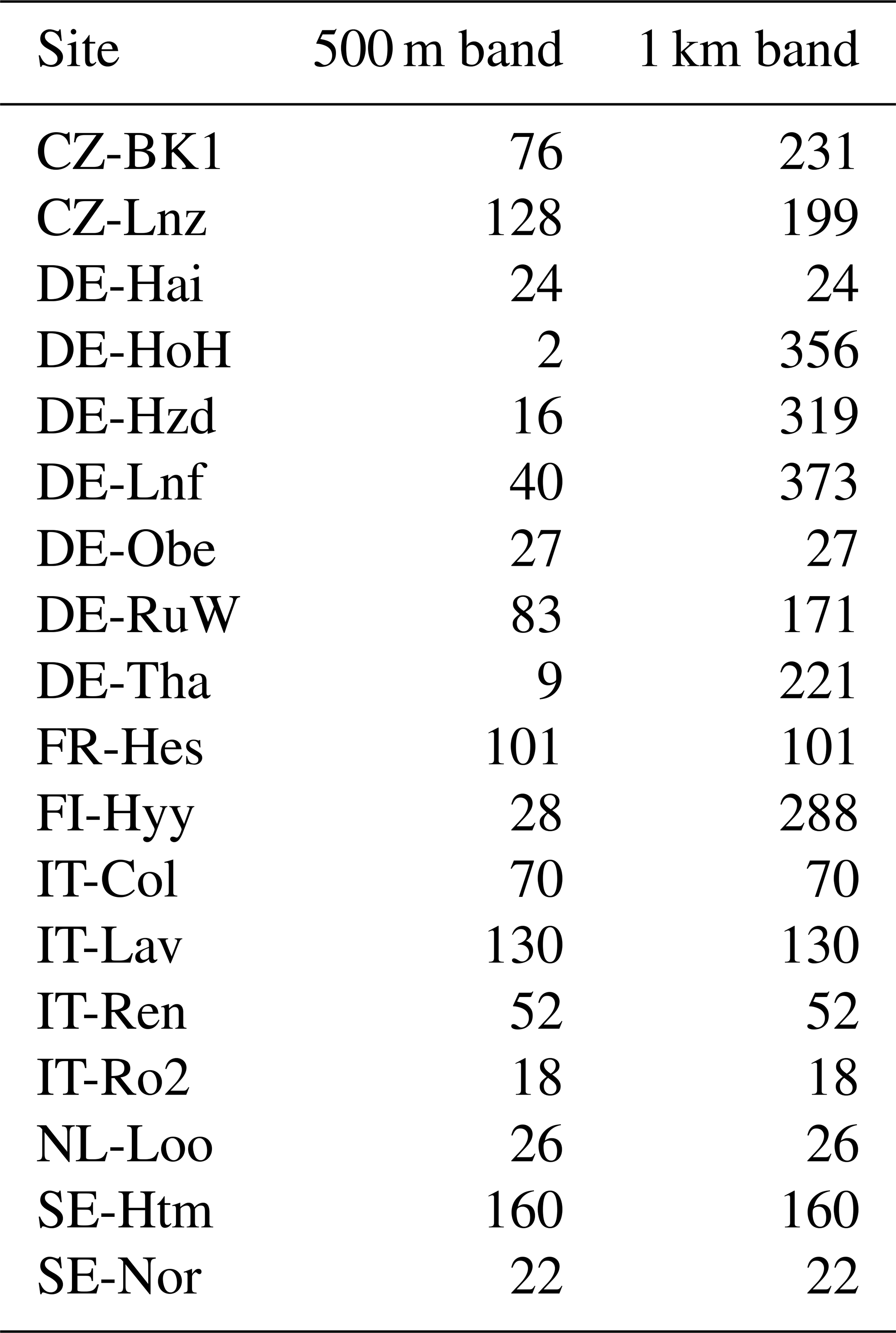
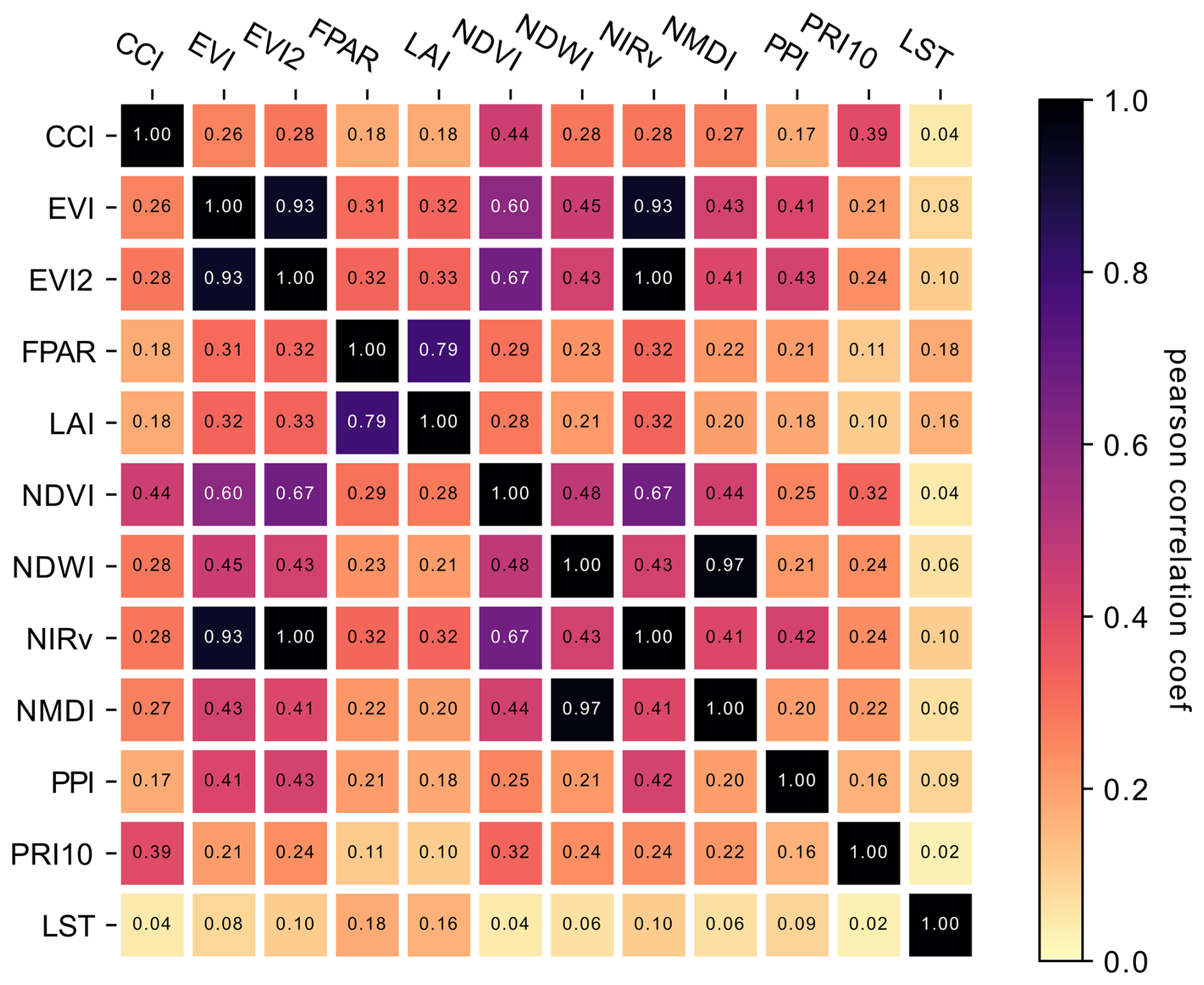
Figure A1 Average within site correlation between each combination of VI z-score time series.

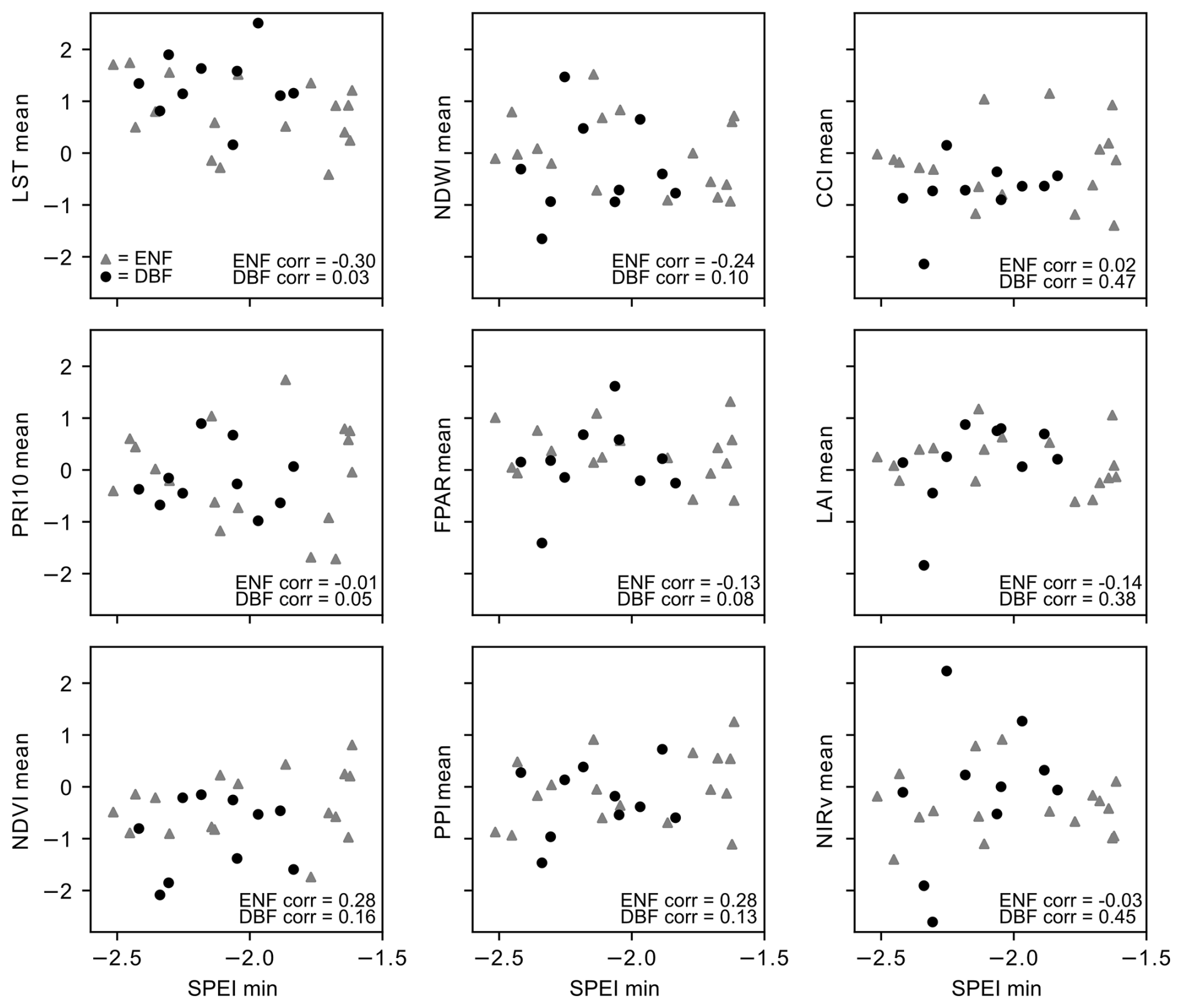
Figure A2 Mean VI z-score during drought versus minimum SPEI during drought for coniferous and broadleaf sites, with spearman's rank correlation coefficients for each forest type.

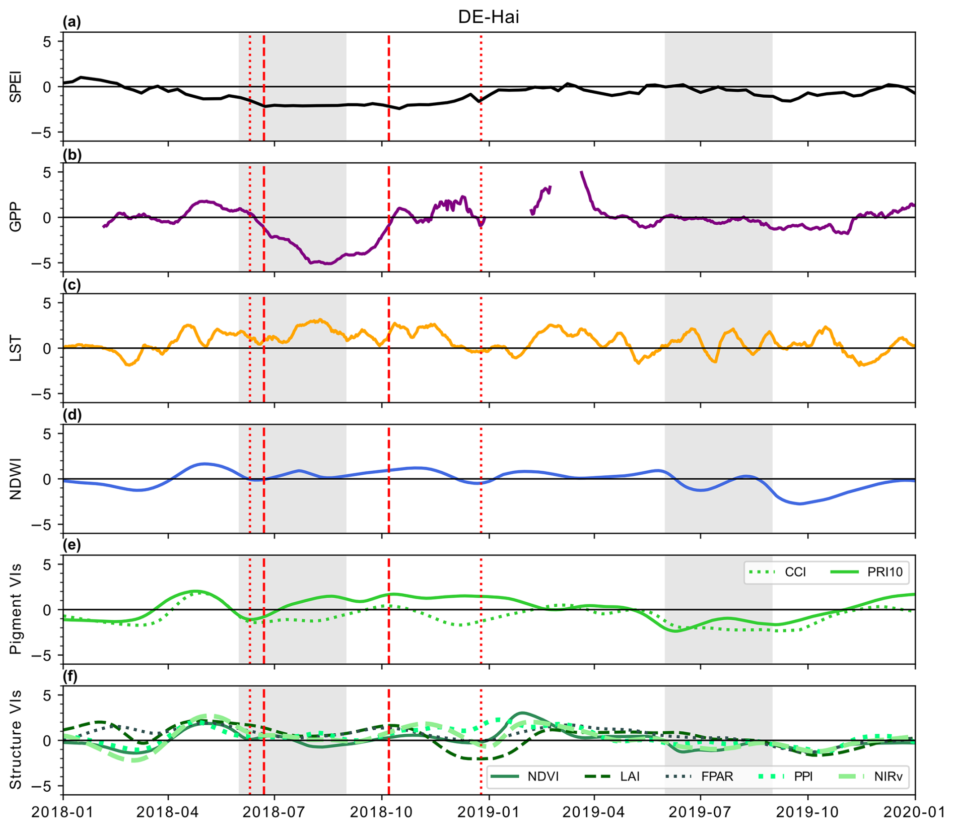
Figure A3 Time series of z-scores during drought and post-drought periods at DE-Hai. Red vertical dashed lines show GPP Date_start and GPP Date_end and vertical red dotted lines show drought start and end dates based on SPEI-3. The grey shaded period shows the peak growing season that is used for the post-drought analysis.

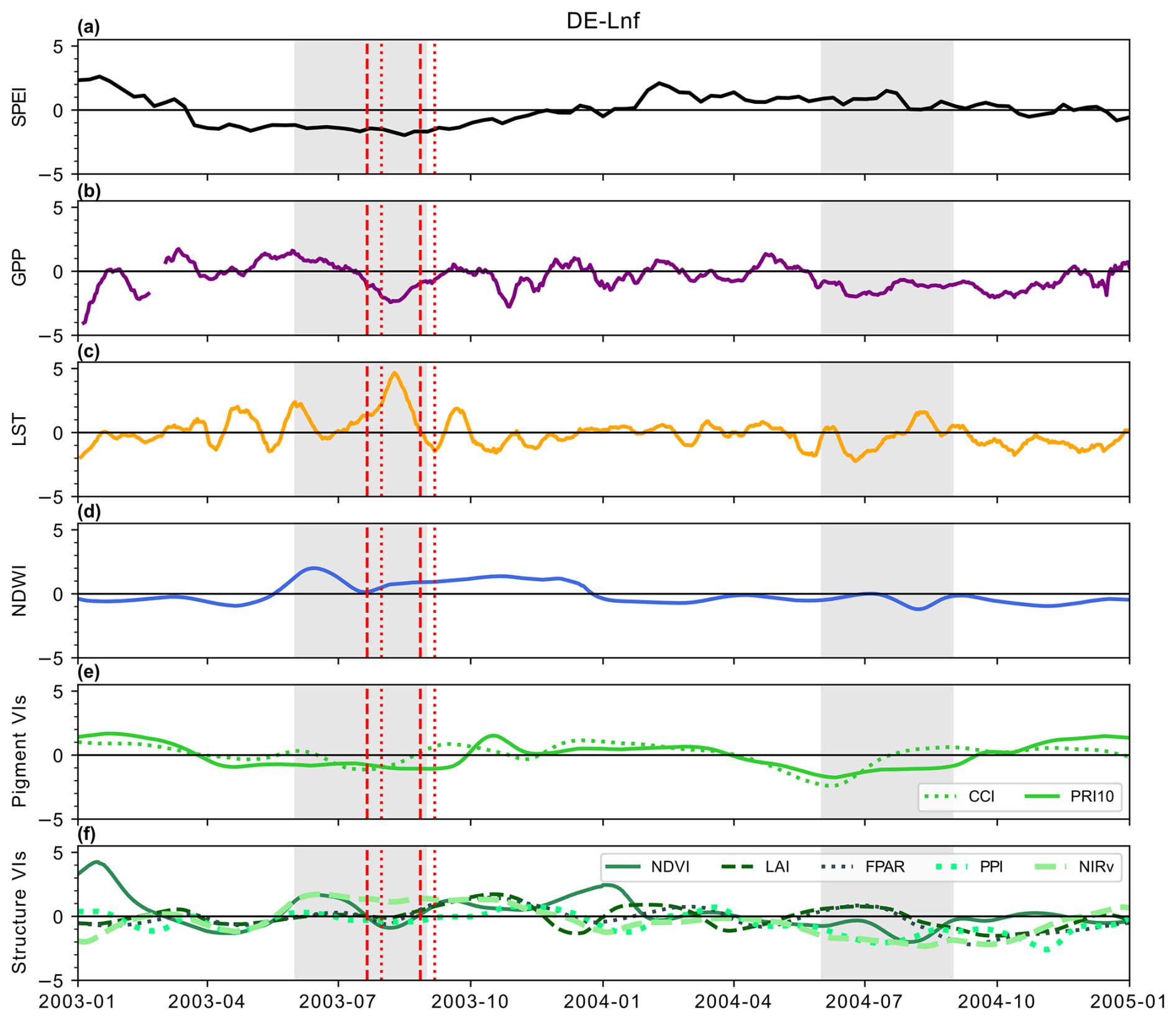
Figure A4 Time series of z-scores during drought and post-drought periods at DE-Lnf. Red vertical dashed lines show GPP Date_start and GPP Date_end and vertical red dotted lines show drought start and end dates based on SPEI-3. The grey shaded period shows the peak growing season that is used for the post-drought analysis.

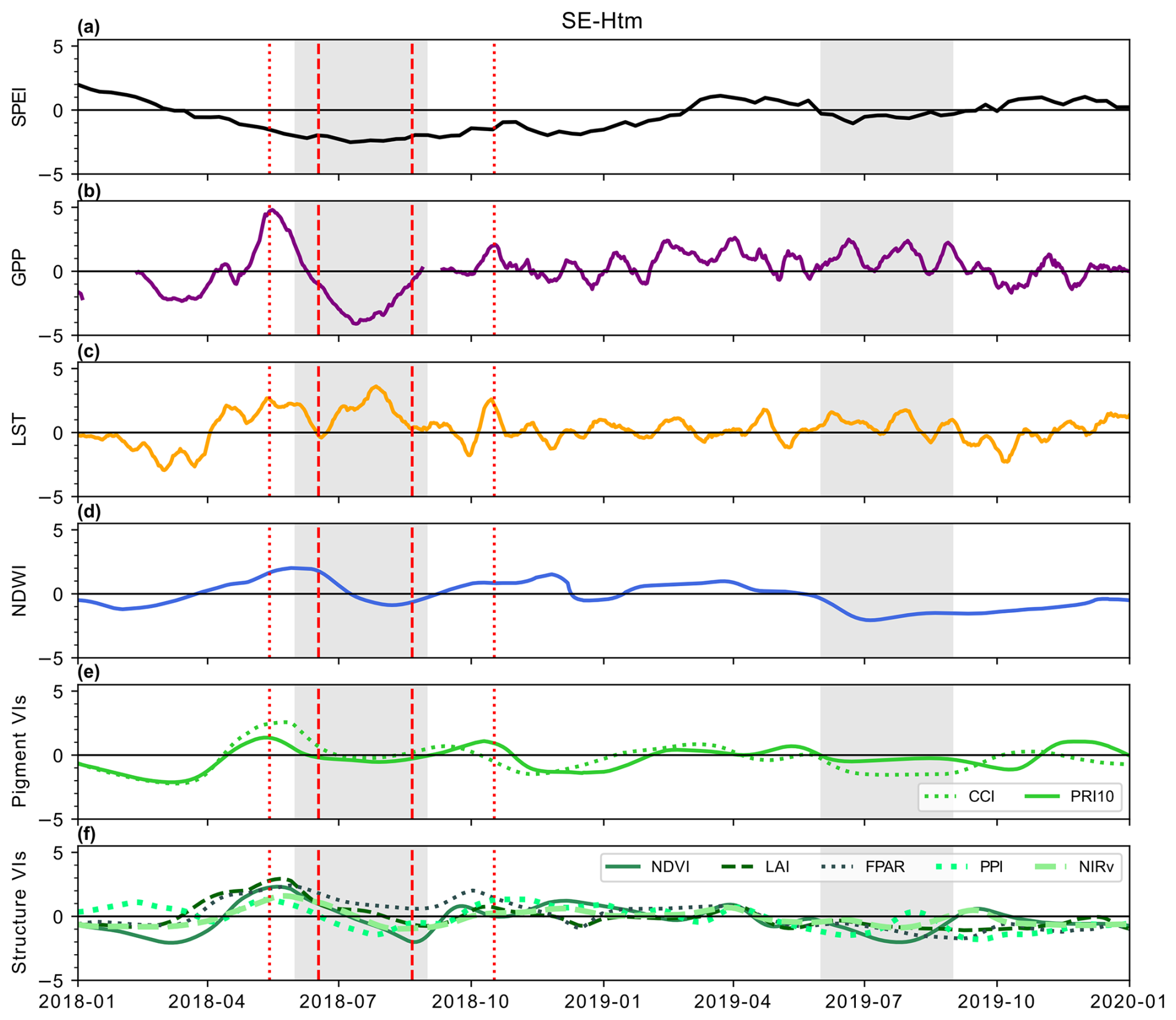
Figure A5 Time series of z-scores during drought and post-drought periods at SE-Htm. Red vertical dashed lines show GPP Date_start and GPP Date_end and vertical red dotted lines show drought start and end dates based on SPEI-3. The grey shaded period shows the peak growing season that is used for the post-drought analysis. The grey horizontal line marks −1 i.e. the threshold we used to define drought response.