Natural wetland methane emissions simulated by ICON-XPP

Natural wetlands emit roughly one third of the global methane emissions, yet their contribution remains highly uncertain. To reduce this uncertainty, we incorporated a fully coupled wetland-hydrology and wetland-methane module into the ICON-XPP Earth-system model and performed a suite of coupled model experiments with prescribed sea surface temperatures spanning 1855–2014. Wetland extent is diagnosed online with a TOPMODEL-based wetland scheme that exploits high-resolution topographic indices, while methane production follows a temperature-dependent anaerobic decomposition formulation calibrated to recent global budgets.

The baseline simulation yields a time-averaged natural wetland methane flux of 182 (154–205) Tg(CH₄) yr⁻¹ for the recent period 2000–2012, in line with the multi-model mean of the global methane budget. Sensitivity experiments reveal that:

1. CO₂ fertilisation is the dominant driver of the observed 12 % increase in emissions since the late 19th century; fixing terrestrial CO₂ at preindustrial levels reverses the trend, producing a net decline in methane flux.

2. Anthropogenic drainage of croplands curtails potential wetland area, especially in the northern extratropics, and offsets part of the CO₂-driven rise in emissions. Experiments that relax drainage or freeze historical land-use increase wetland area by 0.2–0.6 Mm² and raise emissions.

3. The storage of surface water strongly modulates regional precipitation recycling in a coupled model setup, thus significantly altering precipitation in comparison to uncoupled offline experiments.

Overall, the coupled model reproduces observed wetland extents and methane emissions, but suggests that current Earth-system models likely underestimate human-induced hydrological alterations, particularly drainage and water-management practices. Our results underscore the necessity of interactive land-atmosphere coupling and refined hydrological representations for robust projections of future wetland methane feedbacks.

1 Introduction

Methane is – after CO₂ – the second most important greenhouse gas on which humans have a significant direct impact (Zhang et al., 2017; Saunois et al., 2016, 2020, 2025). Since the mid 1980s, the atmospheric methane concentration has been rising by about 7 ppb yr⁻¹ (Lan et al., 2025), with an increasing trend since 2005. Due to its much higher global warming potential compared to CO₂, methane currently contributes almost one third of the anthropogenic climate change (Forster et al., 2021). In combination with the rather short atmospheric lifetime of methane (about 9 years, Saunois et al. (2025)) this could make methane emission reductions an important contribution to reaching the goals of the Paris agreement on a decadal time scale (UNEP, 2021).

Methane is emitted to the atmosphere from a number of marine and terrestrial sources, of which some are anthropogenic, some natural and some natural but influenced by human activities. Emissions from natural wetlands are the largest of the latter type, as they contribute about one third of the total emissions (Saunois et al., 2016, 2020, 2025). Despite estimate uncertainties, it is commonly agreed, that anthropogenic sources have grown larger than the natural ones (Saunois et al., 2025), at least in recent years.

Modeling of wetland methane emissions includes many poorly quantified parameters and processes, which need to be either estimated from observations or modeled interactively. Since methane production takes place under anaerobic conditions, it is closely coupled to the hydrology of the soils, which is used to determine areas where soil conditions are anaerobic. The performance of the current generation of hydrology models is, however, less than perfect (Krysanova et al., 2020; Melton et al., 2013). Furthermore, with few exceptions (e.g., Veldkamp et al., 2018) land surface models used in global Earth System Models ignore active human water management, including such human activities as dam construction, drainage, irrigation and changes in land use that might severely impact the hydrology on local to regional scales (de Vrese et al., 2018; Xu et al., 2024; Chen et al., 2025). Historically, however, such measures have led to the drainage of large wetland areas (Davidson, 2014; Gardner and Finlayson, 2018; Fluet-Chouinard et al., 2023), mainly since the year 1900.

In the high latitudes the presence of (thawing) permafrost further adds uncertainties in wetland estimates (Hagemann et al., 2016; Andresen et al., 2020). The state of the permafrost highly impacts the hydrology of the soils (de Vrese et al., 2023, 2024). Due to small evapotranspiration and the sub-surface runoff partly being blocked by frozen soils, a significant part of global wetlands is located in permafrost areas. Many permafrost-related processes take place at scales far smaller than the resolution of global models (e.g., Rehder et al., 2023) and depend on subsurface developments, which are presently poorly understood and only possible to observe on local scale (Patel et al., 2024). Upscaling these processes to pan-Arctic or even to typical global model grid point scale to obtain robust estimates of soil moisture and wetland area is even more challenging.

Observational estimates of wetland area comes with their own issues and challenges. Zhang et al. (2017) reported a range in the global, annual mean wetland area from five commonly used different observational products from 5.3 to 10.2 Mm² ($\mathrm{1}{\mathrm{Mm}}^{\mathrm{2}}={\mathrm{10}}^{\mathrm{12}}{\mathrm{m}}^{\mathrm{2}}={\mathrm{10}}^{\mathrm{6}}{\mathrm{km}}^{\mathrm{2}}$). Also, large disagreement on the global patterns and annual cycle was reported due to differences in methods, observed periods and original purpose of the data set.

Soil methane production requires available soil organic matter (SOM), anaerobic conditions and sufficiently high temperatures. All of these parameters are estimated by various model components, all of which come with their own uncertainties. Over decades, atmospheric and land models have gained good skills in simulating temperatures and carbon content, whereas the oxygen state of the soils have until recently only received little attention.

Here we present the results of a new implementation of wetland methane emissions based on interactively calculated wetlands in the ICON-XPP (ICON eXtended Predictions and Projections) Earth System Model and the sensitivity to different model assumptions about hydrological management and biogeochemical influences. This will hopefully contribute to a better understanding of the controls on the modeled natural methane emissions, and thus aims to identify and understand uncertainties in the current estimates of wetland methane emissions.

2 Model and development

This study utilizes the ICON Earth System Model, using the ICON-XPP atmosphere model (Müller et al., 2025) and the land surface model JSBACH4 (Schneck et al., 2022). To enable the model to estimate wetland areas and methane emissions, a number of extensions and modifications to the model code have been implemented. These are described in the following subsections.

2.1 Wetlands

In global land-surface modelling the term “wetland” is commonly used in the sense of a hydrological diagnostic, as opposed to an ecosystem characterization: a grid cell (or sub-grid fraction) is labelled a wetland when the simulated water table reaches or exceeds the soil surface, which creates anaerobic conditions that allow methanogenesis. This definition does not imply any change in vegetation type: often, the vegetation cover is prescribed from boundary condition data sets, in our case the from the Land-Use Harmonization 2 (LUH2) land use dataset (Hurtt et al., 2020). This then remains unchanged, regardless of the water-table status. Consequently, a cell that is classified as a wetland in our model may still be labelled “cropland” in the land use map and retain the same crop vegetation. The term “wetland” therefore refers only to the soil-water state that controls methane production, not to the ecological concept of a wetland ecosystem.

We estimated the wetland area fraction using a diagnostic TOPMODEL approach (Beven and Kirkby, 1979), where the compound topographic index (CTI), which describes the relation between the (hydrological) upstream area and the local slope for any point, is used to relate the grid-mean water table to the water-table distribution on the sub-grid-scale topography. The wetland fraction is then assumed to be the fraction of the grid cell where the water table is at or above the soil surface.

The CTI index was obtained from the data set presented in Marthews et al. (2015). However, in order to avoid unrealistically low CTI values that would generate spurious wetlands, we enforce a minimum CTI value of 5.

The calculation of the wetland area does not directly feed back to the soil hydrology. Instead, is assumed that the part of the soils, which are diagnosed as inundated using this approach, are anaerobic. Thereby the wetland extent has an influence on the carbon cycle, which again influences the hydrology (see Sect. 2.2).

We extended the scheme presented in detail in Kleinen et al. (2020) with two improvements:

• The simple piecewise linear estimate of the ice fraction of soil water used in Kleinen et al. (2020) has been replaced by calculations internally in JSBACH's soil hydrology (Ekici et al., 2014; Hagemann and Stacke, 2015). Thus, the freezing and melting of soil water now also influences both the hydraulic conductivity, the energy calculations of the soil and the soil carbon handling.

• In flat areas with shallow soils (e.g., the Sahara), TOPMODEL tends to produce spurious wetlands as a consequence of individual precipitation events, since the shallow soils are rapidly “filled up”. To exclude such artificial wetlands while preserving TOPMODEL's capability to react to changing climatic conditions, an additional dynamic condition to exclude wetlands from very dry areas was introduced: We require that

  $$\begin{array}{}\text{(1)}& {\displaystyle \frac{\stackrel{\mathrm{‾}}{\text{PR}}}{\stackrel{\mathrm{‾}}{\text{AET}}}}>\mathrm{0.3}\end{array}$$

  where PR is precipitation, AET is the equilibrium evapotranspiration, defined by Eq. (2) and an overbar indicates a temporal mean over a “long” period (in this study defined as a running average with an e-folding time of 1 year). This criterion excludes the driest areas while still letting the wetlands develop freely in the rest of the world.

The equilibrium evaporation AET is, following Prentice et al. (1993), defined as:

$$\begin{array}{}\text{(2)}& \text{AET}={\displaystyle \frac{\mathrm{1}}{\mathit{\lambda }}}{\displaystyle \frac{s}{s+\mathit{\gamma }}}\text{NetRad}\end{array}$$

with the rate of change of the saturated vapor pressure: $s=\mathrm{2.503}\times {\mathrm{10}}^{\mathrm{6}}\frac{e^{\mathrm{17.269}\frac{t}{t_{\mathrm{ref}}}}}{t_{\mathrm{ref}}^{\mathrm{2}}}$, the psychrometer constant: $\mathit{\gamma }=\mathrm{65.05}+\mathrm{0.064}t$, the latent heat of evaporation: $\mathit{\lambda }=\mathrm{2.495}\times {\mathrm{10}}^{\mathrm{6}}-\mathrm{2380}t$, $t_{\mathrm{ref}}=t+\mathrm{273.3}$, t is the 2 m air temperature in °C and the NetRad is the net radiative balance in W m⁻².

The diagnostic wetland fraction is evaluated at every model time step (7.5 min). The atmospheric component (ICON-XPP) runs on a triangular C-grid with an R2B4 configuration, i.e., the spacing between grid-cell centers is of the order of 160 km. The CTI field that drives the TOPMODEL calculation is obtained from the global dataset of Marthews et al. (2015) at 15 arcsec (≈500 m) resolution. Thus, the hydrological diagnostic benefits from a high-resolution topographic input, but the underlying climate and land-surface fields are resolved only on the coarse 160 km grid. Consequently, fine-scale features, such as polygonal tundra or palsa complexes in the permafrost region (which have characteristic lengths of a few hundred metres to a few kilometres), are not explicitly represented.

2.2 Wetland methane emissions

The wetland methane production model implementation is adopted from Kleinen et al. (2020), which is based on the approach by Riley et al. (2011). In this model, the decomposition of soil organic matter (SOM) is assumed to occur under anaerobic conditions in the diagnosed grid cell wetland fraction (Sect. 2.1). Due to the anaerobic conditions, decomposition products are not just CO₂, as under aerobic conditions, but both CO₂ and CH₄. The model then transports CO₂, CH₄ and O₂ vertically through the soil column by considering diffusion, ebullition, and plant-mediated transport through aerenchyma, also determining the oxidation of CH₄ in soil layers where sufficient O₂ is present.

In laboratory incubations under strictly anaerobic conditions, SOM mineralisation yields a 50 % CO₂ : 50 % CH₄ split (Conrad, 1999). However, in actual wetland soils this ratio is usually much greater than 1:1, and can vary significantly among different kinds of wetlands (Bridgham et al., 2013). In our model, we therefore assume a significantly lower fraction of CH₄ production, which we furthermore assume to be temperature-dependent in a Q₁₀ formulation. We calibrated this to give a 24 % CH₄ fraction at 295 K and a Q₁₀=1.2 (Riley et al., 2011). This formulation does not distinguish between acetoclastic and hydrogenotrophic methanogenesis, which is the standard approach in most global methane models. Distinguishing acetoclastic from hydrogenotrophic methanogenesis would require explicit representation of substrate availability (acetate vs. ${\mathrm{H}}_{\mathrm{2}}/{\mathrm{CO}}_{\mathrm{2}}$) and is not currently implemented. A recent intercomparison (Xu et al., 2016) reported that 37 out of 40 global wetland-methane models do not separate the two pathways, highlighting that this simplification is common practice, albeit a known source of uncertainty.

Following Wania et al. (2010), we furthermore assume a time- and space-independent reduction of SOM decomposition rate, so that wetland SOM is decomposed with 35 % of the aerobic decomposition rate.

The produced methane, along with CO₂ and O₂, is transported vertically through the soil column via diffusion, ebullition and plant aerenchyma, with process descriptions and parameters adopted from Riley et al. (2011). Depending on the availability of O₂, which can be supplied either via diffusion or via plant aerenchyma, CH₄ may be oxidized partly or completely, also parameterized using a Q₁₀ formulation with a Q₁₀ value of 1.9.

Finally, uncertainty ranges for parameters used in the wetland emission model are sufficiently large that the total emissions (but not the spatial distribution) can be calibrated over a range of wetland area estimates. Thus, we used the CO₂:CH₄ ratio in methane production to calibrate our model to yield global total emissions similar to the Saunois et al. (2016) estimate.

2.3 Anthropogenic drainage of croplands

Historically, many agricultural regions have been drained to remove excess water from fields (Valipour et al., 2020). In the model, this practice is represented by suppressing the diagnostic wetland fraction on all grid cell fractions that are classified as cropland in the LUH2 land use map. Importantly, this drainage flag only suppresses the wetland diagnostics (i.e., the calculation that would label the cell as anaerobic and allow methane production). It does not modify the underlying soil-hydrology equations (soil moisture, infiltration, runoff) nor the carbon-cycle fluxes beneath the crops. The vegetation type therefore remains the prescribed crop (or pasture) throughout the simulation, no transition to natural wetland vegetation (e.g., emergent macrophytes) occurs. Furthermore, the inclusion of drained crops has the advantage, that methane emissions from rice fields (Saunois et al., 2020) are unequivocally attributed as an anthropogenic source and thus fall out of the scope of this study.

2.4 Surface water retention (SWR)

The standard JSBACH model uses the ARNO-scheme (Hagemann and Gates, 2003; Hagemann and Stacke, 2015) to separate rain and melting snow into surface runoff and infiltration into the soil, based on the slope distribution of the grid cell. This scheme ignores that water might pile up in small-scale topographic depressions forming ponds or puddles, from where the water is available for evapo(transpi)ration or later infiltration into the soils. Thus, it may suppress important water and energy feedbacks between surface and atmosphere. It is assumed, that in addition to the micro-topographical effects, this water retention takes place where local soil surface hydraulic conductivity is low. Therefore, the conductivity of these areas is assumed to be equivalent to that of clay, which is the natural soil type with the lowest conductivity. To account for these effects, we implemented the SWR scheme described in detail in Stacke and Hagemann (2012), de Vrese et al. (2021).

It is assumed that the local SWR is a temporary, though possibly repeated, phenomenon compared to the wetlands arising due to saturated soils (Sect. 2.1). The areas inundated by SWR is therefore not counted as wetlands. Due to the lower infiltration in areas with SWR, the soil is comparatively dry, and we assume that these soils stay oxic and therefore do not contribute to the wetland methane production.

3 Setup, experiments and boundary conditions

The experiments were performed with ICON-XPP (Müller et al., 2025) with the extensions discussed in Sect. 2. ICON uses a triangular grid and was in this study run at the R2B4 resolution, which has a cell size of about 25 000 km², roughly corresponding to a resolution of 160 km in a grid with square cells. The atmospheric model used 90 vertical layers, where the upper layer has a pressure of about 1 Pa, and the land model contained 5 soil layers with increasing thickness down to a total soil depth of at most ≈9.5 m, though generally the soil is much shallower.

The model was run using the concentration driven AMIP (Atmospheric Model Intercomparison Project) configuration – that is: the model describes a land surface coupled to an atmosphere, while ocean sea surface temperature, sea ice and greenhouse gas concentrations are prescribed (sea surface temperature and ice using data described in Taylor et al., 2000). Due to the prescription of the greenhouse gases – mainly CO₂ and methane – there is no direct feedback from the terrestrial carbon cycle on to the atmosphere. Thus, this study does not deliver any estimates of atmospheric concentration or lifetime of the methane.

The model was spun up from an initial state without carbon for 160 years, then the slow humus soil pools of the YASSO soil carbon model (Goll et al., 2015; Tuomi et al., 2009) of JSBACH were equilibrated, and the model was spun up for another 50 years. The spinup was done using the vegetation distribution from the LUH2 data set (Hurtt et al., 2020) and greenhouse gas concentrations (GHGs) for the year 1855. During the spinup, the SWR scheme was switched on and crop areas drained as described above.

Table 1 List of conducted experiments. The “Drainage” column indicates whether the diagnostic wetland fraction is suppressed on cropland cells (Yes = drainage active, No = drainage disabled). The CO₂ column only applies to the CO₂ applied to the terrestrial carbon cycle model, while for the radiation calculations, transient CO₂ concentration is always applied. Soil-hydrology and carbon-cycle processes are identical in all experiments.

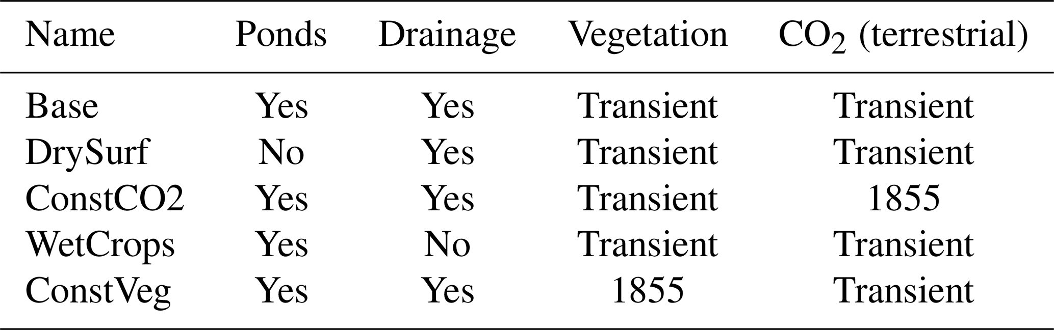
From this spinup, five experiments (Table 1) were branched off, each running from 1855 to 2014, to obtain a best estimate of the natural wetland methane emissions and to explore the influence of different model assumptions:

Base

Fully coupled experiment with SWR active, cropland drainage applied, and transient land-use (LUH2) and CO₂ concentrations.

DrySurf

Same as Base, but surface-water-retention (SWR) disabled.

ConstCO2

Same as Base, but the CO₂ concentration in the terrestrial carbon cycle model is fixed at the 1855 value (while the atmospheric CO₂ used for radiative forcing remains transient).

WetCrops

Same as Base, but cropland drainage is disabled; the prescribed LUH2 crop fraction can become wetland (the vegetation type remains the LUH2 crop, i.e., no shift to wetland plant functional types).

ConstVeg

Same as Base, but the vegetation map is frozen at the 1855 LUH2 distribution; land-use changes (including cropland expansion) are therefore ignored, while the hydrology (precipitation, runoff, SWR) remains fully interactive.

The experiments are stopped in 2014 due to a lack of newer boundary condition data for the atmospheric model. Parts of the analysis therefore concentrate on the period 2000–2012, which was the main focus of Saunois et al. (2016, 2017).

In this study only the data from the terrestrial areas are analyzed, and thus the term “global” hereafter only refers to the terrestrial surface. Furthermore, often the results are discussed separately for a number of regions (Fig. S1 in the Supplement). The most often used regions are the northern extratropics (NXT), defined as the area north of 30° N, and the tropics, which (unless otherwise explicitly stated) – following Saunois et al. (2017) – covers the rest of the world. The latter definition is justified since the southern extratropics only contribute an insignificant fraction of the global wetland area and wetland methane emissions.

The LUH2 data set prescribes 5.8 Mm² of crops in 1855 (3.6 Mm² located in the NXT area). Globally the crop area increase almost linearly to 15.1 Mm² in 2014. However, the NXT contribution stabilizes at about 7.9 Mm² around 1960 and decreases after around 1990 to about 7.1 Mm² in 2014. The increase in crop area is wide-spread in non-mountainous areas of all continents, the exceptions being the north eastern US and Western Europe, where crop areas decrease in the last part of the experiment period. The crop distribution and its changes are important for a proper interpretation of the results from several of the experiments.

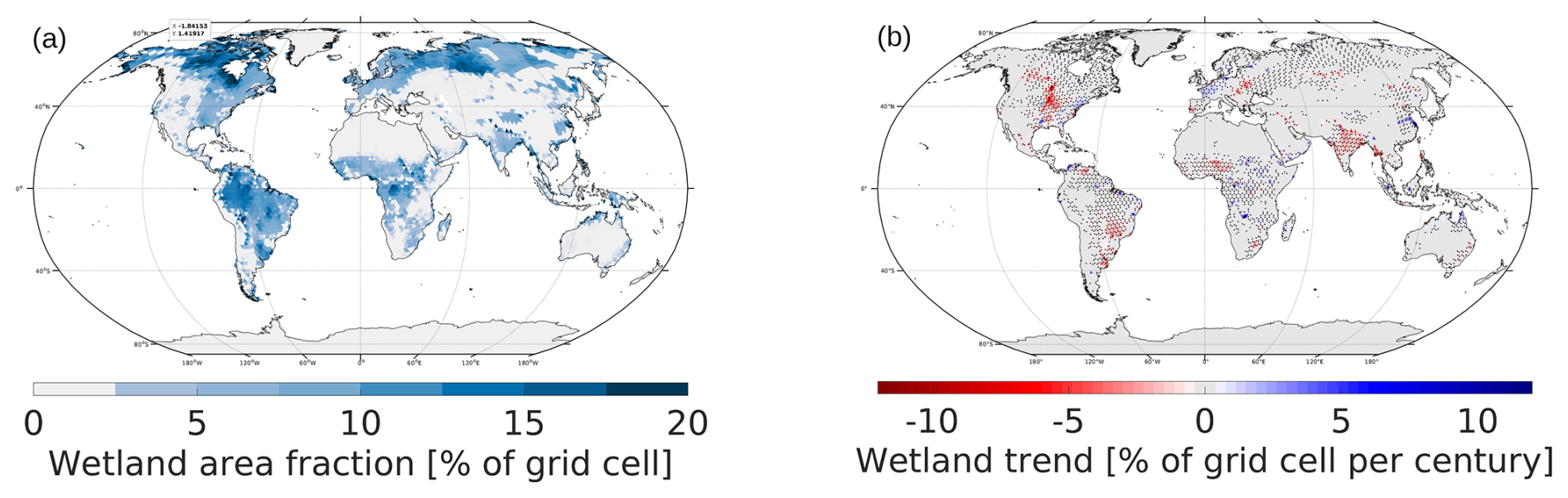
Figure 1 “Base” average distribution of (a) wetland area (% of grid cell area) in Northern Hemisphere summer (JJA) and (b) 1855–2014 wetland area trend of annual means (% of grid cell per century). Black dots mark cells with trends significant at the 95 % level according to Matlab's fitlm function.

4 Results

4.1 “Base” experiment including SWR

The average June–August (JJA) wetland distribution (Fig. 1a) shows the main wetland areas in the tropical rain forests of South America and Africa, as well as in the Hudson Bay area and central northern Siberia. Smaller, but still important, areas are found in India, eastern North America and larger parts of northern Siberia. In addition, some wetlands are found in central western Europe, south-eastern US, Indonesia and eastern China. Roughly, the majority of the Northern Hemisphere summer wetland area is concentrated in two latitudinal bands: the boreal zone (55–70° N), contributing 34 % of the global area, and the tropics (20° S–15° N) with 38 %. The global JJA wetland area is ≈5.2 Mm², with a slight decrease over time (2 % per century). This trend over the entire experiment period, however, hides the fact that the wetlands are only diminishing during the first part of the experiment, while they are growing again at a rate of 7 % per century after 1980. This increase is mainly driven by changes in the NXT area, though the trend also turns the tropics from negative to positive over the course of the experiment. In fact, the wetland area in the NXT region is slightly larger in the later part of the experiment than in the long-term average, and is thus opposing the global decreasing trend (Fig. 4a), leading to an increase in the NXT fraction of the global wetland areas from <30 % in the 1940s to 33 % in the last decade of the experiment (2005–2014). At the start of the experiment, this fraction was about 31.6 %.

The geographical trend distribution (Fig. 1b), shows areas of both increasing and decreasing wetlands: Decreasing wetlands are found in the east-central US, eastern Europe, southern Brazil and India/Bangladesh, while increasing wetlands are found in eastern US and western Europe. In general there is a close relation between the development of cropland (and thus drainage, Fig. S3) fraction and the development of the wetlands.

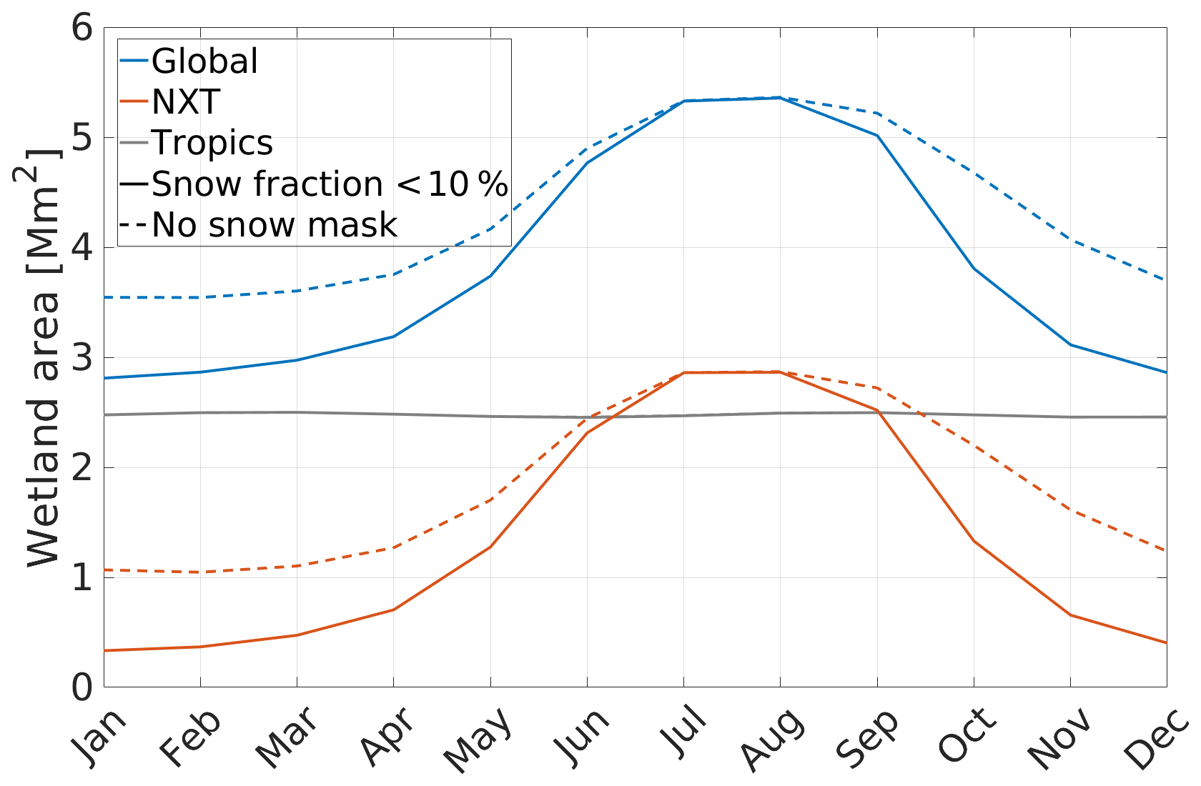
Figure 2 Wetland area annual cycle for the “Base” experiment. Solid lines only include cells with less than 10 % snow whereas dashed lines includes all cells. Blue lines are global values, reddish include only the NXT area (north of 30° N) and the gray line is the “`tropics” (everything south of 30° N). For the tropical area, snow masking does not make any difference.

The average simulated wetland area on non-snow-covered areas in “Base” is ≈3.8 Mm² with a pronounced annual cycle (Fig. 2), ranging from ≈2.8 to ≈5.4 Mm². The year to year variation on the other hand is small (1σ=0.06 Mm²). The annual cycle stems only from the NXT areas, with a maximum in the Northern Hemisphere (NH) summer, June to September, where the northern extratropics are snow free. Though the NXT wetland area in the non-NH-summer increase by up to almost 1 Mm² (November) if no snow masking is applied, the shape of the annual cycle remains. In the annual average, snow is covering ≈0.5 Mm² of wetlands. The lack of an annual cycle in the tropics is to some degree a result of a cancellation of the annual cycles on the difference continents being out of phase (Fig. S2). The rather weak South American wetland annual cycle peaks in April–July and has its minimum in October–January, quite opposite to the somewhat more pronounced annual cycle in Africa, which is the other main tropical wetland region. South East Asia and tropical North America contribute only with very small wetland areas, leaving their influence on the annual cycle diminutive.

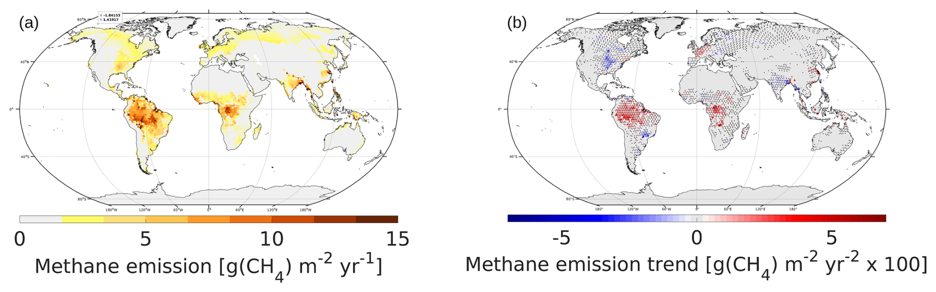
Figure 3 Global distribution of (a) wetland methane emissions in the “`Base” experiment, 1855–2014 average and (b) trend of wetland methane emissions in the “Base” experiment. Black dots mark cells with trends significant at the 95 % level according to Matlab's fitlm function.

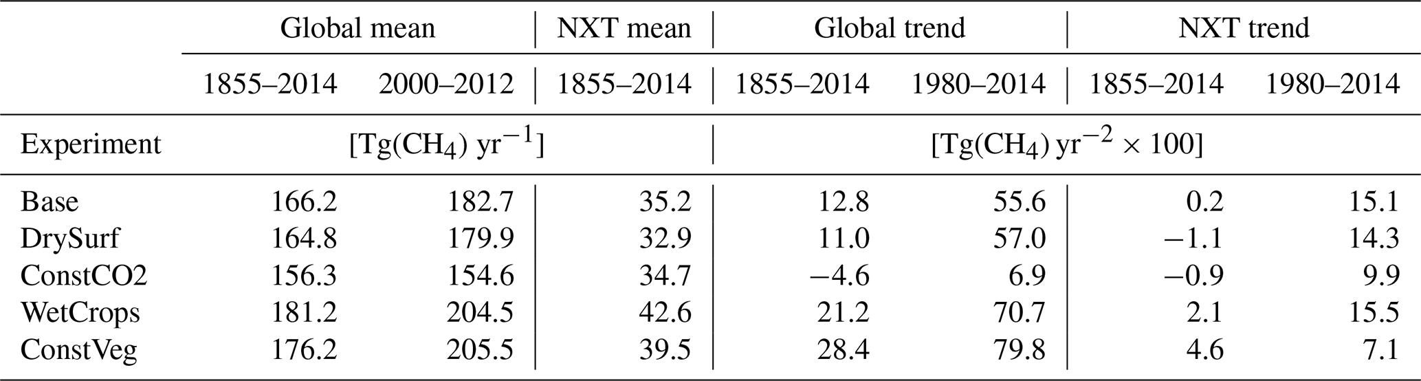
Global wetland methane emissions averaged over the entire experiment period amount to 166.2 Tg(CH₄) yr⁻¹, of which 35.2 Tg(CH₄) yr⁻¹, or about 21 %, are emitted in the NXT area. The rest stems almost exclusively from the tropical rain forest areas in South America, Africa and Indonesia, together with India (Table 3 and Fig. 3a). The relation between the boreal and tropical wetland latitudinal bands is thus quite different with respect to methane emissions: The boreal band contributes only 8 % while the tropical band emits 67 % of global wetland methane. Nzotungicimpaye et al. (2021) report a similar distribution of wetland methane emissions between the boreal and tropical regions using a more microbiologically detailed methane model.

For the period 2000–2012 the global average wetland methane emission is 182.7 Tg(CH₄) yr⁻¹, in close agreement with the multi-model mean presented in Saunois et al. (2016), who report 185 Tg(CH₄) yr⁻¹ for 2003–2012, with a 1σ standard deviation of 21 Tg(CH₄) yr⁻¹.

However, our emissions are more scattered, most pronounced in the Eurasian boreal areas. Higher methane emissions are found in western Europe and southeastern US and lower emissions are found in South East Asia, eastern Africa and the Hudson Bay area. These differences in patterns are quite similar to the multi-model mean of wetland fractions presented in Hardouin et al. (2024).

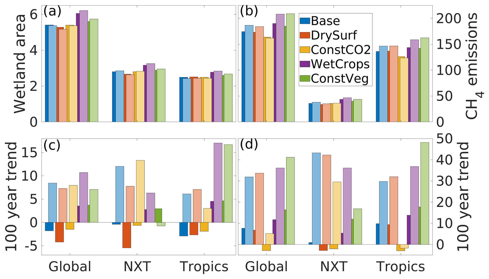
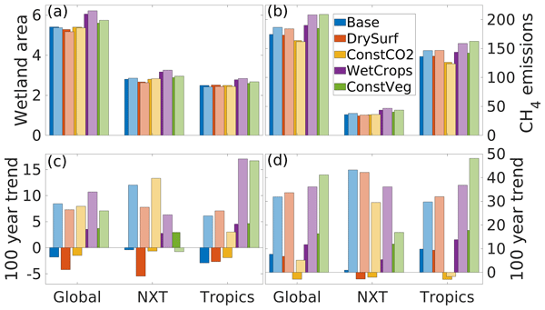
Figure 4 Top panels: NH summer (JJA) Wetland area (in [Mm²]) for areas with ≤10 % snow (a) and annual wetland methane emissions (b, [Tg(CH₄) yr⁻¹]). Bottom panels: 100 year trend ([% of 1855–2014 average]) of (c) annual wetland area and (d) annual wetland methane emissions. Dark (colors exactly matching the legend) partly covered bars represent the entire experiment period (1855–2014), while brighter overlaid bars represent the 1980–2014 period. Colors indicate the different experiments.

The emissions are increasing over time with a trend over the entire experiment of about 20 Tg(CH₄) yr⁻¹ (8 % per century). After around 1980, the trend is about four times as large compared to the entire experiment (Table 3, Fig. 4d). The global increase is mainly driven by increases in the large production areas in South America and Africa as well as Western Europe (Fig. 3b). Decreasing emissions are found in the Central US.

To obtain the standard deviation of the time series, we detrended it by separately subtracting the linear regressions in the time periods 1855–1980 and 1981–2014. The results show very little effect of the exact point of partitioning the regression periods and are virtually identical between the two periods. The standard deviation of the annual average emissions thus obtained is $\approx \mathrm{3.4}\mathrm{Tg}\left({\mathrm{CH}}_{\mathrm{4}}\right){\mathrm{yr}}^{-\mathrm{1}}$.

The emission fraction (the fraction of produced methane that is not oxidised in the soil and thus reaches the atmosphere) is 44.5 % and constant over the experiment period. The emission fraction is geographically very unevenly distributed in complex patterns, where the fractions range from near 0 to almost 80 %. In general, the major methane emitting areas have moderate emission fractions of 30 %–40 %, while hardly any methane escapes from dry areas.

4.2 No surface water retention (“DrySurf”)

Disabling SWR lowers the average wetland area by about 0.1 Mm² (Fig. 4a), with the entire reduction taking place in the NXT area. This mainly happens in the period July–October, and the reduction is almost twice the annual mean. Geographically more specific, the reduction is confined to a narrowing stripe reaching from northeastern Europe into central Siberia and the Mackenzie River basin (Fig. 5a).

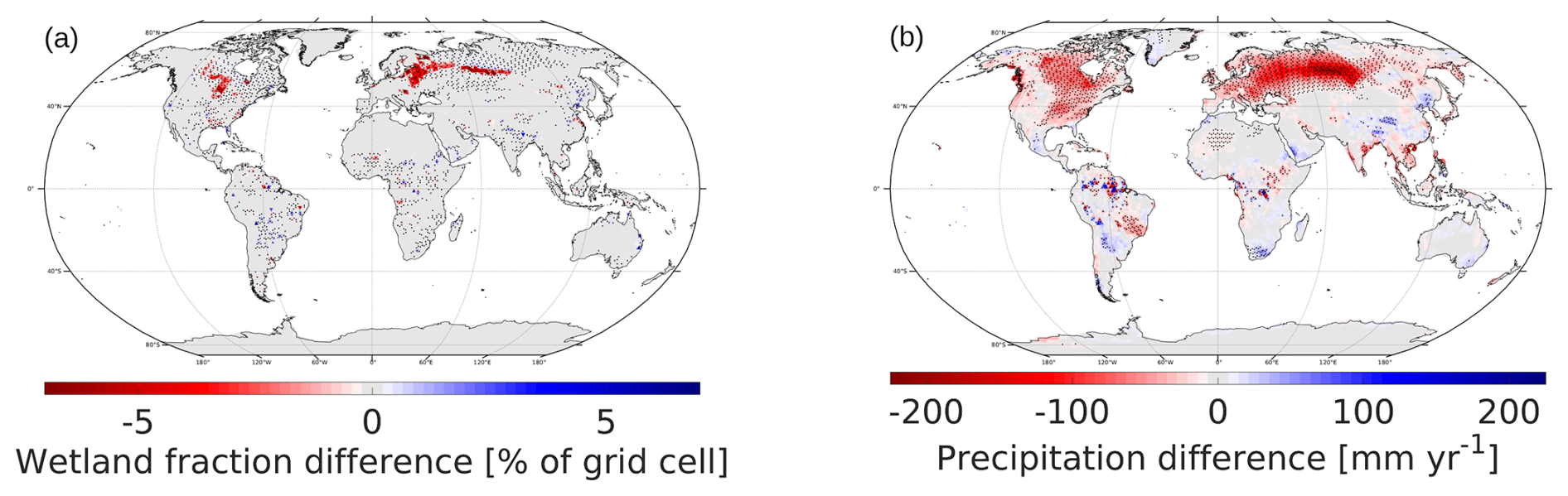
Figure 5 Mean difference in wetland area (a) and annual precipitation (b) between “DrySurf” and “Base” . Black dots mark cells significantly different at the 95 % level between the experiments according to Matlab's ttest function.

The areas of reduced wetlands are within large regions where the precipitation is much lower in “DrySurf” than in “Base” (Fig. 5b). In parts of central Siberia the precipitation reduction is larger than 30 %. Most of the areas with large and consistent precipitation differences are in the areas of the NH jet stream. This indicates a significant shift in the magnitude of moisture recycling through the atmosphere, which is supported by a large decrease of evapotranspiration in “DrySurf” compared to “Base” (not shown).

In “DrySurf” the NXT wetland area decreases by about 7 % per century and thus 5 times faster than in “Base” (Fig. 4c), whereas the tropical wetlands change a bit less in “DrySurf” than in “Base”. The geographical patterns of changing trends between “Base” and “DrySurf” coincide almost exactly with those of the absolute wetland area difference. The average wetland methane emissions (Fig. 4c) from “DrySurf” behave rather similarly to the wetland area: Slightly lower emissions ($\approx \mathrm{2.2}\mathrm{Tg}\left({\mathrm{CH}}_{\mathrm{4}}\right){\mathrm{yr}}^{-\mathrm{1}}$) from the NXT than in “Base” are partly compensated by an even smaller increase ($\approx \mathrm{0.8}\mathrm{Tg}\left({\mathrm{CH}}_{\mathrm{4}}\right){\mathrm{yr}}^{-\mathrm{1}}$) from the Tropics.

In the NXT, the decreasing wetland area trend dominates over the generally increasing trend in methane emissions when looking at the entire experiment: A trend of −3 % per century opposes the tropical trend of +8 % per century. The result is that the global trend is slightly below that of “Base”. Since 1980 this picture is reversed: NXT emissions increase by 42 % per century compared to 30 % in the tropics.

4.3 Neglecting CO₂ fertilisation (“ConstCO2”)

In AMIP experiments with prescribed CO₂, there is no direct feedback from the terrestrial carbon cycle to the atmosphere. Thus, it could be expected that the wetlands in “ConstCO2” would be identical to those in “Base”. This seems to be confirmed by the average wetland area (Fig. 4a), where the two experiments are indeed very close. The trends over the 1855–2014 period, however, are somewhat different, with slightly smaller trends all over the world. In the recent period, the NXT region and the tropics behave very differently: In the tropics the wetland area stagnates with hardly any trend, while the positive NXT trend in “ConstCO2” exceeds that of “Base”. These changes arise as a feedback through changed water-use efficiency of the plants at different CO₂ levels, changing the transpiration. Thus, both water and energy fluxes to the atmosphere are changed, which then trigger different atmospheric responses. Although the global numbers of evapotranspiration are very similar in the two experiments, both the differences in the evapotranspiration itself and its trend show complex regional patterns (Fig. S5).

Keeping the CO₂ concentration constant at pre-industrial levels for the carbon model has a huge impact on the trend of the methane emissions (Fig. 4d). The increasing methane emissions in “Base” are turned into a decrease in the “ConstCO2” and the trend is thus in the opposite direction compared to all other conducted experiments. Only the NXT area has a positive trend in the latter part of the experiment, and this is still smaller than in all other experiments except “ConstVeg” (discussed below). The global carbon litter is – opposite to any other experiment – decreasing after around the year 1900 (Fig. S6). There is still a slight increase in the decomposition of the soil carbon, but only about 5 % of that in the other experiments. That less carbon respires is due to a warmer climate increasing the respiration rate. The reversed trend in the methane emissions in “ConstCO2” reveals, that the trend found in the other experiments is largely due to an enhanced carbon cycle caused by CO₂ fertilisation. Furthermore, different effects on the wetland methane emissions from rising temperatures seems to be canceling each other out, at least on the large scale.

4.4 Increasing potential wetland area: “WetCrops” and “ConstVeg”

Both experiments increase the potential wetland area, but they do so in different ways:

• WetCrops: the drainage flag is disabled, so any cropland cell whose water table reaches the surface is diagnosed as a wetland (hydrologically). The vegetation remains the prescribed crop; no ecological conversion to wetland plants occurs.

• ConstVeg: the LUH2 land use map is frozen at its 1855 state, preventing the expansion of cropland (and the associated drainage) over time. Because the vegetation is fixed, the only driver of wetland change is the hydrological response to climate (precipitation, temperature, SWR). Thus, even with a static vegetation field, the diagnostic wetland fraction can grow or shrink, leading to corresponding changes in methane emissions.

In “ConstVeg” the mean JJA wetland area is 0.2 Mm² larger than in “Base” (Fig. 4a). The increase is entirely due to hydrological inundation of cells that are, for example, forest or grassland in the 1855 land use map. Consequently, the global methane flux rises to 176.2 Tg(CH₄) yr⁻¹ (Table 3), even though the vegetation does not change.

The effect on wetland area of disabling the drainage flag on cropland areas and keeping the vegetation distribution constant at the level of the early industrialization is conceptually the same: The area on which wetlands can exist is increased. In the case of disabled drainage, all crop areas are made available for wetlands, and in the case of constant vegetation distribution, the crop areas are kept smaller, as discussed in Sect. 3. This theoretical behaviour is confirmed by Fig. 4, where average “WetCrops” wetlands exceeds those of “Base” by ≈0.6 Mm² while “ConstVeg” adds ≈0.2 Mm² to the “`Base” wetland area. This increase is essentially equally distributed between NXT and tropics. These two experiments are the only ones having a positive trend in the global wetland area throughout the experiments, somewhat lower in “WetCrops” than in “ConstVeg” and mostly from the tropical area. In the 1980–2014 period, the trends in “WetCrops” are much larger than those of “ConstVeg” in all regions. In the NXT region, the wetlands are even decreasing in “ConstVeg” since they do not profit from the abandonment of croplands in Western Europe and North America. In general, the major difference to “Base” is that “WetCrops” and “ConstVeg” do not participate in the downward wetland area trend, where crops are increasing over the experiment period.

The average methane emissions are also increased compared to “Base”. However, the emissions from “ConstVeg” (176.2 Tg(CH₄) yr⁻¹) are closer to “WetCrops” (181.2 Tg(CH₄) yr⁻¹) than to those of “Base” (166.2 Tg(CH₄) yr⁻¹). The explanation can be found in the methane emission trends, where “ConstVeg” is having the largest trend of all conducted experiments. The reason for the higher trend is that “WetCrops” only changes the wetland area, while no direct changes to the carbon cycle are made in comparison to “Base”. “ConstVeg” changes the vegetation distribution in a way that leaves more space for the most productive vegetation type: the forests. Therefore, more carbon is available for methane production in “ConstVeg” compared to “WetCrops”.

5 Discussion

5.1 Impact of including surface water retention

The significant differences between the “Base” and “DrySurf” experiments highlight the sensitivity of the estimates of wetland extent and thus wetland methane emissions to changes in the soil hydrology. Including SWR dramatically increases the evapotranspiration and thus atmospheric water recycling in some regions. This also has major effects on the fluxes of latent and sensible heat and thus on regional temperature. These feedbacks emphasize the importance of also considering coupled (in this case land-atmosphere) simulations, since such additional water recycling (or lack thereof) is not accounted for in offline, land only, setups. As a result, offline sensitivity studies to changes in, e.g., soil hydrology characterizations may come to wrong conclusions. In similar offline experiments (not shown), forced with the Global Soil Wetness Project Phase 3 (GSWP3) data set (Dirmeyer et al., 2006), the dominating effect of enabling SWR was to decrease the water infiltration into the soil, thus leading to slightly reduced wetland areas and thus lower wetland methane emissions, completely hiding the changes in moisture recycling dominating the coupled experiments.

However, since model estimates of wetland area do not differ by a very large amount between the “Base” and “DrySurf” experiments, and the increase in precipitation tends to occur in regions, where the difference in precipitation between model and observations (Dirmeyer et al., 2006) is relatively small, there is no clear conclusion, whether inclusion of the SWR parameterisation, as in the “Base” experiment, leads to an improvement in model results in terms of wetland areas and wetland methane emissions.

Compared to the TOPMODEL wetlands, the SWR scheme is another way of allowing super-surface water to form, which can be interpreted as wetlands. Both SWR and TOPMODEL-style wetlands arise in areas with high water availability and since both approaches are based on statistical methods, it is impossible to completely separate the two ways of obtaining surface water bodies.

The correlation between the SWR and TOPMODEL-wetland areas in the entire “Base” experiment is ≈0.3 without trend. The assumption that soils below SWR areas are oxic may thus be too simplistic. Since SWR almost exclusively influences North America north-east of the Mackenzie River, north eastern Europe and north western Siberia (Fig. S7), a (partial) lifting of this assumption would enhance the Arctic and Sub-Arctic wetland methane emissions compared to the tropical ones. By assuming that there is no overlap between the SWR and TOPMODEL wetland areas and that annual methane emissions are linearly dependent on the annual mean area with a wet surface, a rough estimate of the effect of the assumption, that the SWR areas do not contribute to methane production, can be obtained. In this case global wetland methane emissions would increase by 42 Tg(CH₄) yr⁻¹ or ≈25 %. This includes an additional 27 Tg(CH₄) yr⁻¹ of emissions from the NXT area, increasing the NXT fraction of the global emissions from 21 % to 30 %. Since the assumptions for this estimate are rather unrealistic, these numbers are, however, regarded as the upper extreme of the consequences of excluding the SWR areas from the methane production.

Table 2 GSWP3 and model precipitation [mm yr⁻¹]. Annual means from year 1901 to 2014. “Tropical”: latitudes between 30° S and 30° N, “SA”: Tropical South America (latitudes 30° S to 12° N), “AF”: Africa south of 30° N, “EA”: East Asia (latitudes 15° S to 20° N, east of 90° E).

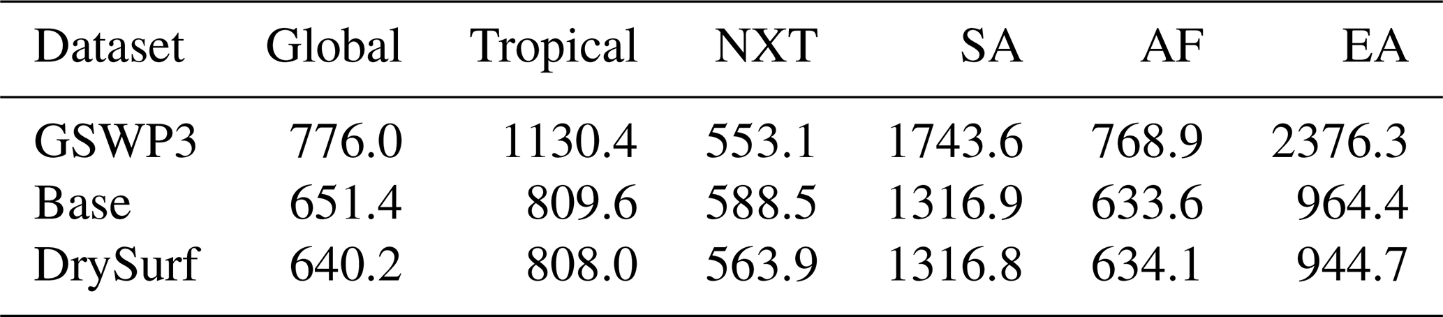
Table 3 Global and northern extratropics (NXT) wetland methane emissions for the entire experiments, the period 2000–2012 (global only, compare to Saunois et al. (2016)) and wetland methane emissions trends for the entire experiments and the last 30 years of the experiments. Trends are given in Tg(CH₄) per year per century.

5.2 AMIP setup versus offline land simulations

Using an AMIP setup introduces an atmospheric variability, which is different from the observed one. Therefore, comparisons of model results to observations and observation-based model results are only possible in a statistical sense over longer periods. In addition, in AMIP setups the atmospheric model may introduce less well-known biases compared to observational data sets. For this study, the most important known atmospheric bias is an underestimation of the tropical precipitation by about 29 % compared to GSWP3 (Table 2). The tropical bias is unevenly distributed between the continents, and is by far strongest over Indonesia and South East Asia, which explains our comparatively low wetland areas and thus methane emissions from this region. The bias distribution agrees with findings of Müller et al. (2025) and seems thus to be a general property of the ICON-XPP atmospheric model. Common wetland products based on observations (GIEMS-2 (Prigent et al., 2020), WAD2M (Zhang et al., 2021)) find a significant seasonal cycle in the tropical wetland area more or less in phase with the northern boreal wetland areas. That in this study essentially no seasonal cycle is found can be attributed to the severe underestimation of south Asian and Indonesian rainfall and thus diminished wetlands in these regions. Therefore, the weak cycle in the Amazonian region can out-weigh the out-of-phase cycles in Asia and Africa, producing a net-zero cycle for the tropics.

5.3 Anthropogenic land use changes including drainage of croplands

The use of land use maps compared to land use transitions (which are currently not implemented in JSBACH4) is known to underestimate the influence of anthropogenic land use changes on the carbon cycle (Wilkenskjeld et al., 2014; Stocker et al., 2014). Specifically the release of soil carbon is underestimated. Therefore, especially in the tropics, where shifting cultivation is a common agricultural practice, the carbon pools may be overestimated. This could also lead to an overestimate of the methane emissions from these regions. Since farmers generally try to avoid wet areas (Valipour et al., 2020), we, however, assume the effect on the methane emissions to be small.

Assuming that all cropland areas in the model are drained is a strong simplification, especially due to the large-scale dynamics and development of agricultural practices. Former cropland areas may be abandoned and become either pastures or completely be given back to nature. This, of course, would not mean that drainage systems are removed, and thus the area drained is likely underestimated by the approach of this study. Also, managed forests, which in JSBACH are regarded as natural vegetation, pastures, and areas of urban expansion may be drained to enhance tree growth, making the land more suitable as grassland or to make the ground supportive for technospheric constructions (Fluet-Chouinard et al., 2023). Again these effects will lead to an underestimate of drained area. On the other hand, not all croplands are drained, either because they are dry enough by nature or because of limited local resources to establish adequate drainage systems. As an example, Valipour et al. (2020) states that in present-day India, only about 10 % of croplands are drained. This will lead to an overestimate of the drained area, but likely not change the simulated wetlands much, since the extra drained area will largely be too dry to regularly become wetlands, anyway. Though Valipour et al. (2020) reports a history of several thousand years of anthropogenic drainage, Fluet-Chouinard et al. (2023) argue that the main wetland area loss due to drainage takes place after 1900 and is still ongoing at a more or less constant rate. Thus, our assumption of drained crops may be most representative for the later part of the simulation period. With the exception of the NXT region in the “ConstVeg” experiment, wetland areas are increasing after 1980 in all of our experiments for both NXT and the tropics. One reason may be different developments in the precipitation and precipitation patterns. GSWP3 and the ICON-XPP atmosphere agree that in the 1980–2014 period, the global (land) precipitation is on average enhanced ($\approx \mathrm{0.48},\mathrm{0.43}$ and 0.32 mm yr⁻² for GSWP3, “Base” and “DrySurf”, respectively). However, the global patterns of increasing precipitation in ICON-XPP correlates better with our simulated wetlands (somewhat better in “Base” than in “DrySurf”), which may thus be enlarged. Nevertheless, it is unlikely that this better pattern correlation alone can explain the trends in wetland area going in different directions in our simulations and observations. It is more likely that we, despite the drainage assumption, largely underestimate the influence of human water management (dams, reservoirs and drainage, also of non-croplands). In total we expect our simulated drained area to be underestimated (and the wetland areas therefore overestimated) in regions with intense and long-lasting anthropogenic influence.

5.4 Wetland area estimates

Data-based estimates of global methane emitting areas are scarce, though a few map-based estimates of wetland extent and remote-sensing estimates of surface inundation are available. Lehner and Döll (2004) estimated the global annual maximum extent of lakes and wetlands based on maps, and show a global extent of methane-relevant wetlands of between 4.5 and 7 Mm², depending on which categories of wetlands are considered relevant for methane. Prigent et al. (2012) developed a remote-sensing-based data set of surface inundation, estimating an annual mean extent of 2.5 Mm², after removal of rice-growing areas based on Monfreda et al. (2008), and a JJA extent of 4.1 Mm². This estimate includes the areas of lakes, reservoirs, and rivers, though, which are not considered methane-emitting areas in our model. Excluding those areas, Zhang et al. (2021) estimate a wetland extent of 4.4 Mm² in the annual mean, with a JJA extent of 5.2 Mm². Finally, Bernard et al. (2025) estimate an annual mean extent of 3.5 Mm² for inundated and saturated wetlands and peatlands, with an annual maximum extent of 7.7 Mm².

Our model estimate yields between 5.3 Mm² in the “DrySurf” experiment and 6 Mm² in “WetCrops”, both for the JJA extent and the 1980–2014 period (Fig. 4), thus determining wetland extents generally in line with data-based estimates. However, a large uncertainty in the estimates of wetlands, and especially methane-emitting areas, has to be acknowledged. The TOPMODEL-based approach we are using determines the extent of (super-) saturated soils, and considers those as methane-emitting. This may, however, underestimate the extent, as some categories, for example peatlands, cannot be considered well in this approach.

Furthermore, the ICON-XPP model shows a precipitation bias over the tropics, specifically in South East Asia, likely leading to too low an estimate of wetland extent for this region in our experiments. Also, JSBACH is not equipped with a detailed river flow model capable of simulating temporary flooding of river flood plains as a consequence of heavy precipitation or snow melt events. Since such wetlands tend to be short-term phenomena, it is questionable, however, whether the soils have time to become anaerobic and thus they would likely not contribute significantly to the wetland methane emissions.

Excluding short-term wetlands in dry areas by applying the dynamic criterion in Eq. (1), instead of a static mask, allows the model to capture the influence of major climatic shifts. This exclusion, the other hand, might also cause spurious trends in wetland area and thus in wetland methane emissions by changing the wetland-allowance mask, either temporarily or as part of a long-term trend. By selecting the required ratio as low as 0.3 (Eq. 1), the bounds of where wetlands are permitted are located far away from where major wetlands are predicted. Thus, the wetland methane emissions and their trends are likely not influenced by the details of this masking.

5.5 Wetland methane emissions

In the “ConstCO2” experiment the trend in wetland methane emissions is much smaller than in “BestGuess”. Over the entire experiment period it is even negative, following the downward trend in wetland area. This suggests that the main driver of the trend found in all other experiments is an accelerated carbon cycle stemming from CO₂ fertilisation. This contradicts the findings of both McNorton et al. (2016) and the WETCHIMP model ensemble (Melton et al., 2013), who attribute their trend to a temperature-driven increase of wetland area and microbial methane production rates.

For the period 2000–2012 the trend in global wetland methane emissions is about 0.4 Tg(CH₄) yr⁻², of which 75 % stem from the tropics. This is higher than the numbers presented in Saunois et al. (2017), who report a multi-model mean of 0.2 Tg(CH₄) yr⁻², and about 10 % of a trend of 2.2 Tg(CH₄) yr⁻² from top-down inversions attributed to non-anthropogenic sources. Since the productivity in JSBACH is known to be comparatively sensitive to changes in the atmospheric concentration of CO₂, which is the driver of our trend in methane emissions, it appears likely that our predicted wetland emission trend is at the high end.

The basic TOPMODEL assumption defining wetlands as areas with super-saturated soils (i.e., the water level is at least reaching the surface) and using the wetland fraction as a measure of the soil oxygen content are simplifications, which can only serve as a first guess. For instance soils, where the root zone of macrophytes is saturated, may be anoxic. Thus, though the soil column as a whole is not saturated, such areas could be a source of methane, mainly since produced methane may bypass the upper (oxic) soil layers through aerenchyma. On the other hand, soils take time to become anoxic after being inundated. Depending on the state of the soil at inundation, this may take hours to weeks (Patel et al., 2024), and the anaerobic area could thus potentially be overestimated by assuming all wetland soils to be anoxic. Further, wetland areas may have very different and highly heterogeneous methane production and emission rates, as shown for Arctic ponds by Rehder et al. (2023).

Of course, the tropical precipitation bias reducing our tropical wetland area tends to decrease the importance of the tropical wetland methane emissions. There are, however, also effects which draw in the other direction: In this study, we accounted only for the conversion of contemporary organic matter to methane, while in reality an additional source may be added from the huge amount of ancient organic carbon stored in the thawing permafrost (Hugelius et al., 2014), as well as from degrading peatlands (Hugelius et al., 2020), since we include no explicit peatland model such as HIMMELI (Raivonen et al., 2017). Ekici et al. (2019) found that incorporating micro-scale ground subsidence following permafrost thaw will increase the wetland fraction and thus methane emissions. Both these effects would enhance the importance of the Arctic regions in the global methane budget. Even though our wetlands are in general smaller, the modeled NXT fraction agrees with the more detailed wetland methane model of Nzotungicimpaye et al. (2021).

5.6 Offline versus online simulations

Offline (stand-alone) land-surface simulations are valuable for isolating the response of wetland hydrology to prescribed climate, but they cannot capture feedbacks such as (i) moisture recycling that modifies precipitation patterns, and (ii) vegetation-mediated changes in surface energy fluxes. Conversely, online coupled simulations may inherit atmospheric biases (e.g., the tropical precipitation deficit in ICON-XPP) that propagate into the wetland response. Therefore, both experimental designs are complementary: offline experiments help to diagnose process sensitivities, while online experiments are required to assess the full climate-wetland feedback loop.

6 Conclusions

Sub-models for coupled wetland dynamics and wetland methane emissions have been built into the ICON-XPP Earth System Model. The resulting wetland distributions, when accounting for precipitation biases from the atmospheric model, align very well with observations. Additionally, the estimates of wetland methane emissions agree well with published values. Sensitivity studies were done to quantify effects of certain model assumptions and anthropogenic influences on methane emissions from natural wetlands.

Agricultural development encompassing both the changes in farmed area and cultivation practices, is the dominant anthropogenic factor controlling the natural wetland methane emissions by controlling the potential wetland area. Until around 1980, this resulted in a global decrease in wetland area, counteracting the general trend of increasing wetland methane emissions. In contrast to the simulations presented here, observations suggest that global wetland area is still decreasing as a consequence of human actions, indicating that anthropogenic influences on the global soil hydrology are underestimated in the current generation of Earth System Models.

The second-most significant human-influenced factor affecting wetland area and their methane emissions is the increase in atmospheric CO₂ concentrations. This rise accelerates the carbon cycle through CO₂ fertilisation. This, however, does not significantly impact the wetland area. The temperature effect of rising atmospheric CO₂ concentration does not substantially affect wetland area and methane emissions.

Changes in the model description of the surface hydrology, including the implementation of surface water retention, have the potential to significantly alter land-atmosphere water and energy fluxes on the regional scale and thus need to be evaluated using coupled setups.