Using deep learning to assimilate sun-induced fluorescence satellite observations in the ISBA land surface model

Accurate representations of the surface and vegetation are critical for simulating the terrestrial CO₂ cycle in response to climate and meteorological conditions. To meet this challenge, an increasing number of satellite missions are being launched which can monitor vegetation conditions and biomass. One is the Copernicus Sentinel-5P mission, which carries the TROPOMI instrument and retrieves Sun-Induced Chlorophyll Fluorescence (SIF). As an indicator of plant photosynthetic activity, SIF can provide critical information for evaluating and parameterising gross carbon flux dynamics in surface models. This study aims to assimilate TROPOMI SIF data into the ISBA (Interactions between Soil, Biosphere and Atmosphere) land surface model developed by Meteo-France, with the objective of directly correcting the representation of Leaf Area Index (LAI) and Gross Primary Production (GPP). To achieve this, we have developed a dedicated observation operator that links the modelled LAI to the TROPOMI SIF daily product. This neural network (NN) operator was developed using deep learning and was trained using observations over Europe. This operator achieved good accuracy, was implemented in a land data assimilation system (LDAS), and was used to assimilate TROPOMI SIF in ISBA using a sequential simplified extended Kalman filter. Specific experiments were conducted to study the assimilation process over the Ebro basin in Spain. This area is known for its irrigated croplands, which are not well represented by ISBA. Some experiments assimilate TROPOMI SIF, some assimilate a Copernicus Land Monitoring Service (CLMS) LAI 10 d product, and some assimilate both. This provided us with a useful point of reference for improving the vegetation simulation. Following SIF assimilation, LAI representation improved across the domain, highlighting heavily irrigated croplands. The gross primary production (GPP) derived from the analysis is closing the gap between the simulated and observed values, though a marked difference remains. When compared with other assimilation experiments, assimilating SIF alone provides a similar benefit to standard assimilation of a CLMS LAI product on LAI and GPP. The best improvements to the LAI and GPP results come from co-assimilating TROPOMI SIF with the CLMS LAI product, which combines the advantages of high-frequency SIF observations and robust 10 d LAI assimilation.

1 Introduction

Monitoring the carbon cycle in near real time at city, regional and national scales helps decision-makers track the effectiveness of environmental policies in the context of climate change mitigation and emission reduction efforts (Horowitz, 2016). One of the main efforts at the European level was to develop and maintain a new operational monitoring and verification support capacity (CO₂MVS) for the carbon cycle. It has been demonstrated that the natural carbon flux of the land surface is the most uncertain component of the carbon budget (Agustí-Panareda et al., 2022; Friedlingstein et al., 2025). Near real-time monitoring requires a joint analysis of the water and carbon cycles. Incorporating new observations of soil moisture and vegetation variables, such as Leaf Area Index (LAI), into land surface models can enhance the precision of these systems (Sabater et al., 2008; Albergel et al., 2020). One promising type of observation is the remote sensing of sun-induced chlorophyll fluorescence (SIF) in vegetation  (Bolhar-Nordenkampf et al., 1989; Moya et al., 2004). Solar radiation flux is absorbed by chlorophyll, enabling photosynthesis and fuelling biological fluorescence in the near-infrared and far-red regions of the spectrum (Berry, 2018). SIF has distinctive spectral maxima that can be extracted from Top of Atmosphere (TOA) radiance measurements taken in space (Köhler et al., 2015; Joiner et al., 2016). Recently, SIF was retrieved on the large swath of the Copernicus Sentinel-5 Precursor instrument: TROPOMI (Köhler et al., 2018; Guanter et al., 2021). It provides a daily estimate of SIF in the near-infrared spectrum. SIF observations have been shown to correlate strongly with LAI, gross primary production (GPP) and other vegetation monitoring variables (Leroux et al., 2018; Butterfield et al., 2023). It has also been used to optimise the parameterisation of vegetation simulation models by Bacour et al. (2019).

In order to improve operational monitoring of vegetation, Garrigues et al. (2026) assimilated the reprocessed 8 d SIF retrieval from raw TROPOMI data into the IFS land surface model developed at ECMWF on a global scale. In this study, we propose to constrain simulations from the ISBA (Interactions between Soil, Biomass and Atmosphere) land surface model, which is developed at Météo-France and available via the SURFEX (SURFace EXTernalisée) platform (Masson et al., 2013; Decharme et al., 2013), by assimilating the raw daily TROPOMI SIF retrievals instead of the 8 d TROPOMI SIF product used by Garrigues et al. (2026). Unlike Garrigues et al. (2026), the ISBA land surface model simulates LAI. As the SIF is not explicitly simulated by ISBA, a new observation operator is required to map the model variables into observation space. A process-based SIF observation operator is complex, requiring computational resources to accurately solve the radiative processes and calibration to reduce associated uncertainties. This makes it difficult to implement such an observation operator in an operational system. An alternative machine learning-based operator for SIF could be more suitable. TROPOMI SIF provides daily global retrievals, which will serve as our database for developing and training a neural network observation operator. Corchia et al. (2023) have successfully achieved the assimilation of new observations in the ISBA land surface model using a neural network observation operator for ASCAT (ESA Advanced Scatterometer) backscattering observations. We adapted this methodology and applied it to the assimilation of TROPOMI SIF.

This article describes the design of the regional deep learning observation operator for SIF measurements and its use in a sequential assimilation process to constrain simulations produced by the ISBA land and vegetation surface model within the SURFEX platform. The benefits of assimilating TROPOMI SIF data will be evaluated in the Ebro basin. This specific region was chosen because the land surface model does not represent the heavily irrigated croplands resulting from field management. TROPOMI SIF assimilation can correct this. The next section presents the datasets used to train the observation operator and evaluate it later on. The land data assimilation and the deep learning operator are then described in the Methods section. Section 4 is dedicated to the results, beginning with an evaluation of the observation operator and the various assimilation strategies for TROPOMI SIF alongside different observation errors. Section 5 discusses the complementarity of LAI and TROPOMI SIF observations in a co-assimilation framework, and outlines limitations in GPP representation when assimilating only TROPOMI SIF. The final section draws conclusions.

2 Datasets

2.1 Domain

All the datasets for the training of the observation operator are extracted on a large regional domain. The database domain covers Europe, extending from 26° W to 46° E and from 28 to 72° N. The grid is uniform and regular with a resolution of 0.1°. This domain is the same domain as that used by Hamer et al. (2026). Grid cells of vegetation are selected within this domain using the ECOCLIMAP-II land cover classification (Faroux et al., 2013), which is available in SURFEX. Figure 1a illustrates the most common vegetation type found within each grid cell. In ISBA, urban areas are considered as bare rock. As such, urban areas are also displayed as bare rock in Fig. 1. In terms of low vegetation, Europe is dominated by C3-grassland and C3-crops, with forests of mixed deciduous and coniferous trees in higher latitudes. The zoom in Fig. 1b is on the Ebro and Rio Segre basins in Spain. This region is well known for its heavily irrigated crop fields, which are usually difficult to model accurately.

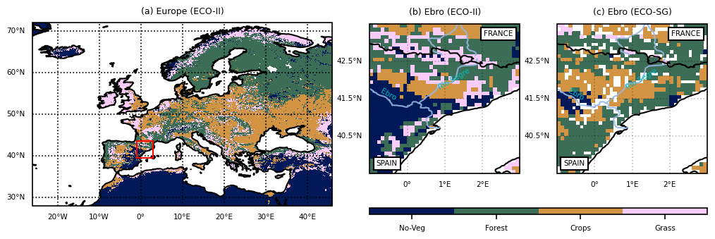
Figure 1 Dominant Plant Functional Type according to land use maps. (a) Domain Europe with ECOCLIMAP-II [26° W to 46° E, 28 to 72° N], the delimited area in red represents the Ebro basin subdomain. (b) The Ebro basin subdomain [1° W to 3° E, 39.5 to 43.5° N] with ECOCLIMAP II. (c) The Ebro basin subdomain with ECOCLIMAP-SG. Four surface types are shown: grass (C3 grassland, C4 grassland), crops (C3 croplands, C4 croplands, flooded crops), forest (deciduous broadleaf forest, coniferous needleleaf forest, evergreen broadleaf forest), No-veg (bare soil, rocks, snow and ice, peat and wetlands).

2.2 SIF database

TROPOMI SIF is a high-level product obtained from the atmospheric reflectivity data collected by the Sentinel-5P SWIR instrument as part of the TROPOSIF project (Guanter et al., 2021). The distributed data ranges from May 2018 to December 2021 for the project, but the same process is now operational on the online data portal that distributes the product. Here, we used the data from the TROPOSIF project. Sentinel-5P operates on a heliosynchronous orbit and, with a swath of 2600 km, passes over a given region at least once a day (Veefkind et al., 2012). The nadir measurement crosses the equator at 13:30 local solar time, achieving a resolution of 7 km ×3.5 km. The retrieval process involves statistically modelling TOA radiances over vegetation while excluding the signal induced by the underlying bare surface. The MODIS2018 database (Friedl and Sulla-Menashe, 2015) is used to identify areas of vegetation that are relevant for SIF retrieval. Using prior knowledge of the SIF spectrum, the algorithm extracts the SIF-related part of the TOA radiance signal (Guanter et al., 2015). This process ensures that the distribution of TROPOMI SIF observations is centred on zero over grid cells where there is only bare soil (i.e. where MODIS classifies the land as having no vegetation). This means that non-physical negative values for TROPOMI SIF can occur. TROPOMI SIF instantaneous estimates are computed according to a spectral window between 743 and 753 nm. The estimates are robust to cloud contamination. Alongside these instantaneous estimates, the Level-2 TROPOMI SIF product provides a corrected value according to day length and solar angle at a given latitude (Köhler et al., 2018). We will be using the raw SIF retrieval from this corrected Level-2 TROPOMI SIF.

In this study, since our model domain is defined on a 0.1° resolution regular grid, the raw SIF retrievals were aggregated onto our model grid. Only all positive instantaneous measurements for a given day covering a grid cell in the domain are aggregated to provide a value for that grid cell.

2.3 LAI and GPP observations

To complete the training and evaluation of vegetation monitoring, we considered two additional types of vegetation observation: LAI and GPP. The LAI satellite products used here are provided by the Copernicus Land Monitoring Service (CLMS). LAI-GEOV1 (Baret et al., 2013) is an observation-driven product with a resolution of 1 km, based on measurements from the SPOT-VGT satellite (from 1999 to 2014) and the PROBA-V satellite (from 2014 to June 2020). It provides an estimation of LAI at a global scale every 10 d denoted thereafter as LAI-V1. To align with our daily TROPOMI SIF product, the LAI maps undergo linear time interpolation. Due to instrument issues or excessive cloud cover during observations, random local missing values are displayed on each global map. Time interpolation is only performed between two consecutive LAI observations of the same grid cell separated by 10 d. If an LAI observation is missing, the gap is not filled. As in previous studies (Albergel et al., 2010; Barbu et al., 2011; Corchia et al., 2023, among others), LAI observations are aggregated to the spatial resolution of the model grid points using an arithmetic average, provided that the LAI observations cover at least 50 % of the grid cell area. As the LAI-V1 product was discontinued in June 2020, the CLMS LAI raster at a resolution of 300 m will be used instead. This is derived from Sentinel-3 OLCI (Ocean and Land Colour Instrument) measurements. This provides data every 10 d and is spatially and temporally interpolated in the same way as the LAI-V1 product and, is referred to as LAI-300 thereafter.

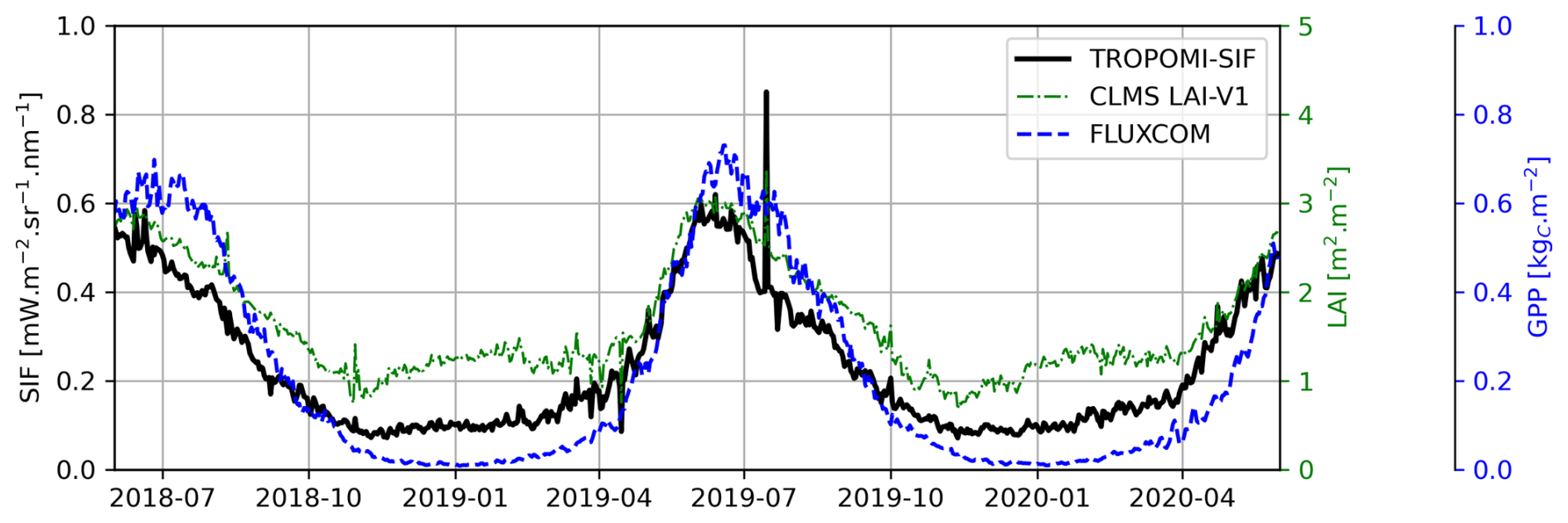
For the GPP, we used the most recent global FLUXCOM-X in V0 product (Jung et al., 2020; Nelson et al., 2024). This provides daily estimates of GPP at a quarter-degree resolution across the globe from 2018 to 2021. The time series of the three observation products are displayed in Fig. 2. All of the displayed observations are from the European domain; the GPP from FLUXCOM remains at its original resolution. The expected seasonal cycle is present in all products. The high-frequency variability in median LAI and TROPOMI SIF values is due to changes in data masking by clouds and filtering applied to both datasets. The isolated spike in mid-July 2019, which is present only in the TROPOMI SIF and LAI-V1 datasets, is a rare case in which the Iceland area is the only region observed due to common masking.

Figure 2 Time series of the median value of LAI (green), SIF (black) and GPP (blue) observed over the domain shown in Fig. 1a.

3 Methods

3.1 ISBA land surface model

Throughout this study, we use the version 8.1 of the SURFEX platform (Masson et al., 2013) to model the surface. To model the soil-plant system, we use the ISBA land surface model. Soil moisture and LAI are computed independently for different plant functional types (PFTs). Twelve PFTs are used and distributed according to land use maps. The ISBA model (Noilhan and Planton, 1989; Noilhan and Mahfouf, 1996) is used in the A-gs configuration (Calvet et al., 1998), where A stands for CO₂ assimilation by the leaves and gs stands for the stomatal conductance simulated by the model. ISBA-A-gs considers the functional relationship between stomatal aperture and photosynthesis under well-watered conditions, as described in the biochemical A-gs model proposed by Jacobs (1994) and Jacobs et al. (1996). For drier conditions, the model also includes a representation of soil moisture stress, as well as two dedicated drought responses: one for herbaceous vegetation and crops, with specifications for C3 and C4 types (Calvet, 2000), and one for forest vegetation (Calvet et al., 2004). Further details on the ISBA-A-gs can be found in Gibelin et al. (2006). Below the surface, the soil is discretised vertically for both soil temperature and soil moisture. The multi-layer soil model uses a diffusion scheme to solve the one-dimensional Fourier law (Decharme et al., 2011) for soil temperature, and a mixed form of the Richards equation (Richards, 1931) for soil moisture. The ISBA models' simulations can be inaccurate when compared with observations. We address these inaccuracies by assimilating observations into the model.

3.2 Land Data Assimilation system

To constrain the ISBA-A-gs model simulations, we assimilate observations sequentially using the global Land Data Assimilation System (LDAS-Monde) described in Albergel et al. (2017). This process involves updating the control variables in the ISBA model by minimising discrepancies between the variables and observations, and between the variables and a prior estimate. In our case, the control vector comprises the LAI and the soil moisture in the different layers. The results from this process is known as the “analysis”. We use a simplified extended Kalman filter (SEKF, Mahfouf and Bilodeau, 2009). Thereafter, the control vector will be referred to as x_i, where the subscript denotes the temporal step, which corresponds to one day since the assimilation is performed daily. The analysis update equation at t of the Kalman filter from the background control vector at t−1 is as follows:

$$\begin{array}{}\text{(1a)}& {\displaystyle }{\mathit{x}}_t^{\mathrm{b}}={\mathcal{M}}_{t-\mathrm{1}}\left({\mathit{x}}_{t-\mathrm{1}}^{\mathrm{a}}\right)\text{(1b)}& {\displaystyle }{\mathit{x}}_t^{\mathrm{a}}={\mathit{x}}_t^{\mathrm{b}}+\underset{\mathrm{Increment}}{\underbrace{{\mathbf{K}}_t({\mathit{y}}_t-{\mathcal{H}}_t({\mathit{x}}_t^{\mathrm{b}}\left)\right)}},\end{array}$$

where the superscripts “a” and “b” stand for analysis and background respectively. y_t represents observations. The operators ℳ and ℋ are respectively the land surface model (i.e. ISBA) and the linear observation operator that maps the control vector into the observation space. The Kalman gain K_t is defined at time t as follows:

$$\begin{array}{}\text{(2)}& {\mathbf{K}}_t={\mathbf{BJ}}_t^{\top }(\mathbf{R}+{\mathbf{J}}_i{\mathbf{BJ}}_t^{\top }{)}^{-\mathrm{1}}\end{array}$$

where B and R are error covariance matrices characterizing the background and observation errors respectively. The operator J is the Jacobian matrix of the partial derivatives and is defined according to Eq. (3).

$$\begin{array}{}\text{(3)}& {\mathbf{J}}_t={\displaystyle \frac{\partial \mathcal{H}\left({\mathit{x}}_t^{\mathrm{b}}\right)}{\partial \left({\mathit{x}}_{t-\mathrm{1}}^{\mathrm{a}}\right)}}={\displaystyle \frac{\partial \mathcal{H}\left({\mathcal{M}}_{t-\mathrm{1}}\right({\mathit{x}}_{t-\mathrm{1}}^{\mathrm{a}}\left)\right)}{\partial \left({\mathit{x}}_{t-\mathrm{1}}^{\mathrm{a}}\right)}}\end{array}$$

This Jacobian is computed using finite differences. This is achieved by perturbing each component of the control vector defined by Rüdiger et al. (2010). To simplify the extended Kalman filter, its background error covariance and the observation error covariance matrices are assumed to be diagonal. These covariance values are fixed for a given assimilation window of 24 h, as detailed in Mahfouf et al. (2009); Albergel et al. (2010); Barbu et al. (2011); De Rosnay et al. (2013); Albergel et al. (2017); Fairbairn et al. (2017, among others).

The background state is computed from the analysis performed over the previous 24 h assimilation window, see Bonan et al. (2020) for more details. Assimilation are thus cycled over a 24 h period like described in the scheme displayed by Fig. 3. As example, the baseline LDAS configuration at Meteo-France involves assimilating LAI 10 d retrievals with a fixed relative observation error of 20 % (Hamer et al., 2026; Bonan et al., 2020; Albergel et al., 2020, among others). Since the purpose of assimilation is to bring the model closer to the observations, the difference between the analysis and the observations in observation space – denoted as residuals – should be smaller than the difference between the prior simulation and the observations – denoted as innovation. LAI assimilation does not require a new observation operator to be defined, but SIF assimilation does. In order to assimilate SIF, we have designed a new observation operator based on a neural network that maps ISBA control variables to TROPOMI SIF retrievals.

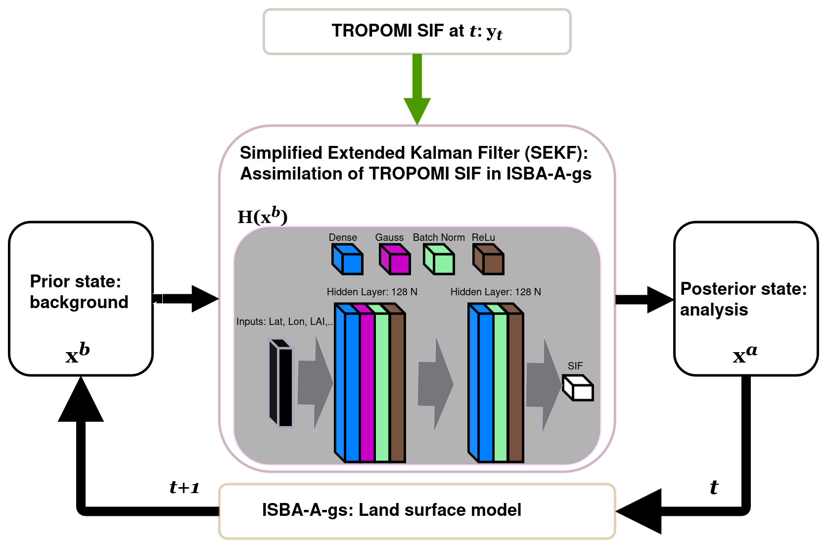
Figure 3 Schematic representation of the neural network architecture integrated in the assimilation framework. x^b and x^a are respectively the background and the analysis and represents 8 control variables. The observation assimilated y_i at the ith cycle in this schematic representation is TROPOMI SIF.

3.3 Neural network observation operator

For training and evaluation purposes, all areas covered by ocean, water, snow or lakes, or lying above 1500 m a.s.l., or where bare soil, rock, snow or ice are most prevalent according to ECOCLIMAP-II, are removed. Grid cells with no LAI or SIF observations, and grid cells where the soil surface temperature fell below 277.15 K according to the SEEDS project analysis (LOBELIA, 2024) and Trimmel et al. (2023), are also excluded to prevent the inclusion of frozen vegetation and soil.

Here, we address a regression problem that can be solved using a simple feed-forward neural network (NN) for nonlinear regression. This strategy produced good results for the assimilation of ASCAT backscattering coefficient σ₀ in  Corchia et al. (2023), where NNs were trained independently for each grid cell. However, in this study, we will train a single neural network that can be applied to any grid cell. A feed-forward neural network’s basic architecture comprises an input layer, one or more hidden layers of neurons, and an output layer, which provides an estimate. After some testing, we found that the configuration comprising two hidden layers of 128 ReLu-activated neurons strikes the best balance between computational cost and accuracy. As our problem is a regression problem, our output layer comprises a single neuron with linear activation as shown in Fig. 3. We added a Gaussian noise layer to the first hidden layer, before the activation layer, to reproduce the effect of a noisy activation layer that would be applied to the inputs. This helps to avoid overfitting during training and enables the duplication of the inputs for data augmentation. This Gaussian layer is only involved during the training process. We expect the neural network to provide smoother estimates than the observations and to filter out the inherent noise of the TROPOMI SIF data. We added a batch normalisation layer at the end of each hidden layer to regularise the learning process.

The distribution of TROPOMI SIF values resembles a log-normal distribution, with a mode close to zero (see Fig. S1 in the Supplement). In order to prevent the neural network from making non-physical negative predictions and to widen the SIF distribution, it will be trained to estimate the SIF_l variable. This is the SIF transformed by the strictly increasing function given in Eq. (4a). We applied the following strictly increasing function Eq. (4a) to the TROPOMI SIF values to predict SIF_l. To reconstruct SIF estimates from the neural network outputs, the reverse equations Eq. (4b) are used.

$$\begin{array}{}\text{(4a)}& {\displaystyle }{\mathrm{SIF}}_l=\mathit{\{}\begin{array}{ll}\ln \left(\mathrm{SIF}\right),& \text{if}\mathrm{SIF}\le \mathrm{1}\\ \exp (\mathrm{SIF}-\mathrm{1})-\mathrm{1},& \text{if}\mathrm{SIF}>\mathrm{1}.\end{array}\text{(4b)}& {\displaystyle }\mathrm{SIF}=\mathit{\{}\begin{array}{ll}\exp \left({\mathrm{SIF}}_l\right),& \text{if}{\mathrm{SIF}}_l\le \mathrm{0}\\ \ln ({\mathrm{SIF}}_l+\mathrm{1})+\mathrm{1},& \text{if}{\mathrm{SIF}}_l>\mathrm{0}.\end{array}\end{array}$$

For the loss function, we compare the label value and the prediction of the neural network according to an Huber loss, which follows Eq. (5). This loss behave mainly like the usual mean square loss while being less sensitive to outliers due to its more linear behaviour for extreme differences.

$$\begin{array}{}\text{(5)}& \mathcal{L}({\mathrm{SIF}}_l,x)=\mathit{\{}\begin{array}{ll}\frac{\mathrm{1}}{\mathrm{2}}({\mathrm{SIF}}_l-H(x){)}^{\mathrm{2}},& \text{if }|{\mathrm{SIF}}_l-H(x\left)\right|\le \mathrm{1}\\ \left(\right|{\mathrm{SIF}}_l-H\left(x\right)|-\frac{\mathrm{1}}{\mathrm{2}}),& \text{if }|{\mathrm{SIF}}_l-H(x\left)\right|>\mathrm{1}.\end{array}\end{array}$$

After a thorough study exposed in the Sect. S1 of the Supplement, the neural network takes only as predictors the DOY, LAT, LON and the observed LAI-V1. This configuration ensures that SIF assimilation can easily adapt to any land surface model and remain robust in the face of improvements to these models. The NN was trained for at least 100 epochs to ensure convergence of the 18 000 estimated weights, as shown in Fig. S5 of the Supplement. The full data range is from 1 June 2018 to 31 December 2021; however, LAI-V1 is only available until June 2020, meaning that the training and testing datasets include only dates between the beginning of June 2018 and the end of May 2020. The first year (i.e. 1 June 2018 to 31 May 2019) was used for training. Within the training period, 40 % of the training database is effectively used for the training of the weights, while the remaining 60 % is used to validate the neural network internally during the learning process. This division is randomised to avoid spurious temporal correlations. The “training” and “validation” splits are used to check for possible overfitting during training. Even when using only 40 % of the training dataset, the neural network is trained using 14 million input/output pairs. As Fig. S5 in the Supplement shows, using more data for training did not increase accuracy. Data augmentation involves duplicating random training values until the size of the dataset is double the original size. The test dataset, which is unknown to the training model, is used to evaluate the model's ability to generalise. This ranges from 1 June 2019 to 31 May 2020. In summary, the neural network learns using data from one year and is then evaluated using data from a different year.

To evaluate thereafter the NN, we will compute the Pearson's correlation coefficient (ρ_p) between the reconstruct SIF from the NN and the observed one, the root mean square error (RMSE) between the reconstruct SIF and the observation, the mean bias of the difference between the reconstruct SIF and the observed SIF (i.e. experiment minus observations), the unbiased root mean square error (ubRMSE) to have an estimation of the standard deviation of the differences and the extreme values of the differences. These criteria will be computed for both the training and testing sets to ensure that there is no overfitting.

3.4 Assimilation setup over Ebro basin

To limit the computational cost, the assimilation TROPOMI SIF will be done only on a small area of 40×40 cells within the European domain displayed in Fig. 1b. This domain encompasses the Ebro and Rio Segre basins in Spain. This area comprises heavily irrigated croplands which are usually not accurately simulated by the land surface model (Jarlan et al., 2023; Lunel et al., 2024). Our approach aims to enhance the simulation of these irrigated areas by assimilating TROPOMI SIF data. The assimilation period runs from 1 January 2018 to 31 December 2021. The SEKF from the LDAS model assimilates the observations daily at 13:00 UTC. While the NN operator was trained using European data screened according to ECOCLIMAP-II, the land cover map used for the assimilation experiments was defined using ECOCLIMAP-SG (Calvet and Champeaux, 2020). This land cover is more recent and accurate than the ECOCLIMAP-II land use map, and Fig. 1c shows that it displays more croplands over the Ebro domain.

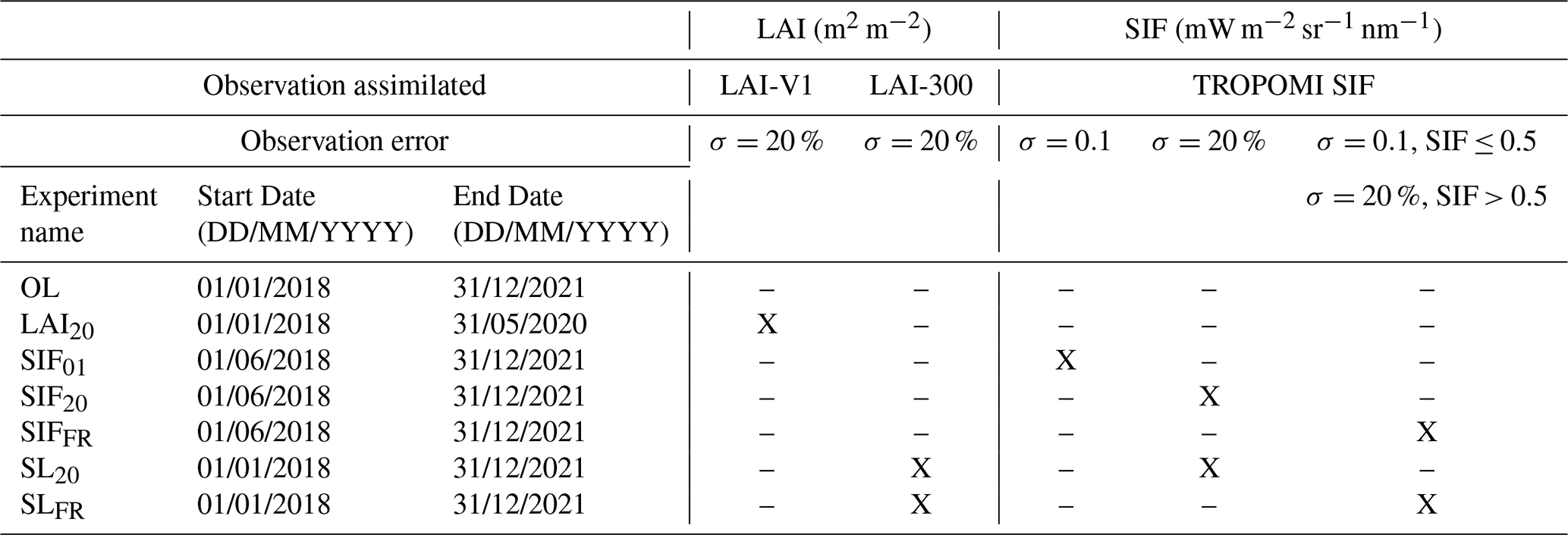
In order to evaluate the benefits of assimilating TROPOMI SIF data, we ran an open-loop simulation from 1 January 2018 onwards. This provides a reference point for determining the impact of assimilating SIF data, and it will henceforth be referred to as the “OL experiment” in Table 1. Another reference experiment we use is the baseline experiment, which is referred to as the LAI₂₀ experiment in Table 1. The LAI₂₀ experiment will use the LDAS to assimilate LAI-V1 from 1 January 2018 to June 2020, and provide a state-of-the-art analysis to evaluate the specific benefits of assimilating SIF data. The initial conditions were spun up for 20 years and shared by these to reference experiment and all SIF assimilation experiment described thereafter. To determine the amount of SIF observation error to consider, three different experiments are run with three different amounts of error: (i) 0.1 mW m⁻² sr⁻¹ nm⁻¹, (ii) 20 % of relative error, and (iii) a combination of the previous two errors with a fixed error of 0.1 mW m⁻² sr⁻¹ nm⁻¹ for SIF values below 0.5 mW m⁻² sr⁻¹ nm⁻¹ and 20 % of relative error for values above 0.5 mW m⁻² sr⁻¹ nm⁻¹. This configuration will be denoted FR thereafter. Two additional experiments are run to test the co-assimilation of TROPOMI SIF and CLMS LAI 300 m raster for two different values of the SIF observation error and 20 % of relative error for the LAI (Barbu et al., 2011). All experiment configurations are summarised in Table 1.

Table 1 Overview of the assimilation experiments conducted for TROPOMI SIF on the Ebro basin domain. The table indicates the name of the assimilation experiment (Experiment name), the assimilation of the LAI and which dataset (LAI) with an observation error of 20 %, the assimilation of TROPOMI SIF (SIF) with wich observation error (σ) used.

The efficiency with which TROPOMI SIF is assimilated into ISBA using the NN operator will be assessed by computing the root mean square error (RMSE) and the Pearson’s correlation coefficient between the analysed fields and the observed values (i.e. LAI and GPP). To ensure the statistical relevance of these evaluations, a p-value is computed using a Fisher's test when calculating the various Pearson correlations. Any results with a p-value greater than 0.01 are removed.

4 Results

4.1 Validation of the observation operator

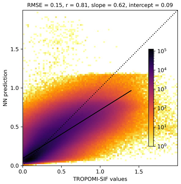
The correlation between TROPOMI SIF and the estimate from the operator is above 0.8 and the RMSE on SIF is around 0.15 mWm⁻² sr⁻¹ nm⁻¹ as displayed in Table 2. However, the neural network's range is smaller than that of the TROPOMI SIF. Both the values closest to and farthest from zero are miss-estimated by the NN. To improve our understanding of the neural network's behaviour, we evaluate its performance on specific TROPOMI SIF samples. We also check whether the neural network's behaviour is sensitive to the range of TROPOMI SIF values and the dominant PFT, in order to ascertain whether it learns features relating to vegetation distribution and phenology. Table 2 shows the results for both the training and test datasets to detect any overfitting.

Table 2 Evaluation of the neural network over the train and the test dataset. The percentiles are taken from the range of TROPOMI SIF values. RMSE, ubRMSE, Bias, Median, Minimal and maximal values of the differences between estimated SIF and observation are given in mW m⁻² sr⁻¹ nm⁻¹. Bold values are when the sample is equal to the full dataset (Train or Test).

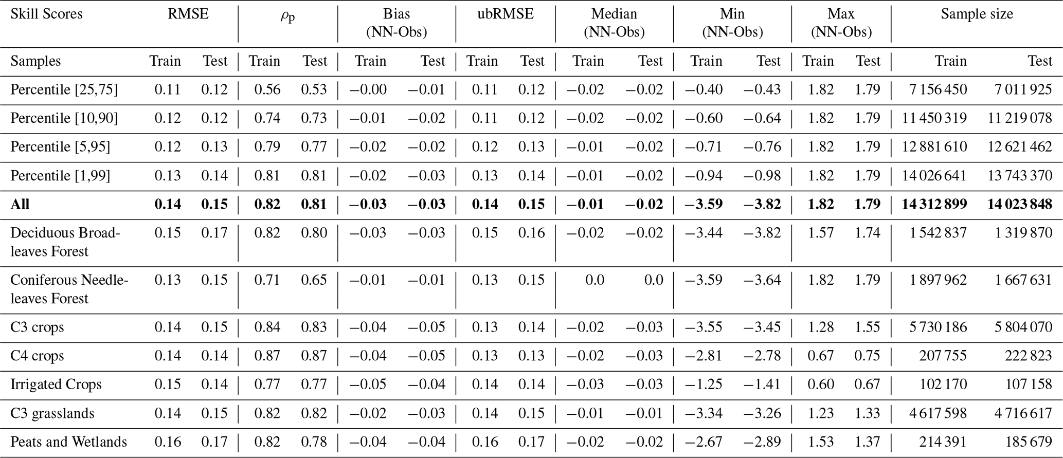
As can be seen in bold in Table 2, the overall skill score values obtained for the training and test datasets are similar. This suggests that if there is any overfitting, it is limited. Comparing the skill scores for the different percentiles of TROPOMI SIF values, we can see that, as we consider more data from the edges of the distribution, the bias (i.e. the mean of the NN estimates minus their observed counterparts), the RMSE and the correlation all increase. This indicates that the neural network disregards minor variations around the mean TROPOMI SIF value. This behaviour is to be expected due to the use of Huber loss during training, which focuses on minimising the RMSE. Furthermore, when the values are farther from the mean, the neural network follows this change, thereby increasing the correlation. However, the bias also increases with the SIF value, thus increasing the RMSE.

A negative bias means that the neural network is underestimating the TROPOMI SIF value. This is particularly evident for the largest SIF values. The neural network performs better over areas where crops, grasslands and deciduous broadleaf forests are most prevalent. Coniferous needle-leaf forests (CNF) and flooded areas (irrigated crops) seem to present more difficulty, as Table 2 shows.

The differences in behaviour depending on the SIF values and the PFT motivate us to verify whether some spatial properties need to be considered in our evaluation. Figure 4 shows the local values of the root mean square error (RMSE), correlation, number of available comparisons and normalised root mean square error (NRMSE) for the entire test dataset. The normalisation is done by the TROPOMI SIF value. The correlation is above 0.8 in the area south of 60° N. This is due to the number of observations available in the region. The northern area is not observed for more than half of the year by TROPOMI around the winter period and less LAI observation are available.

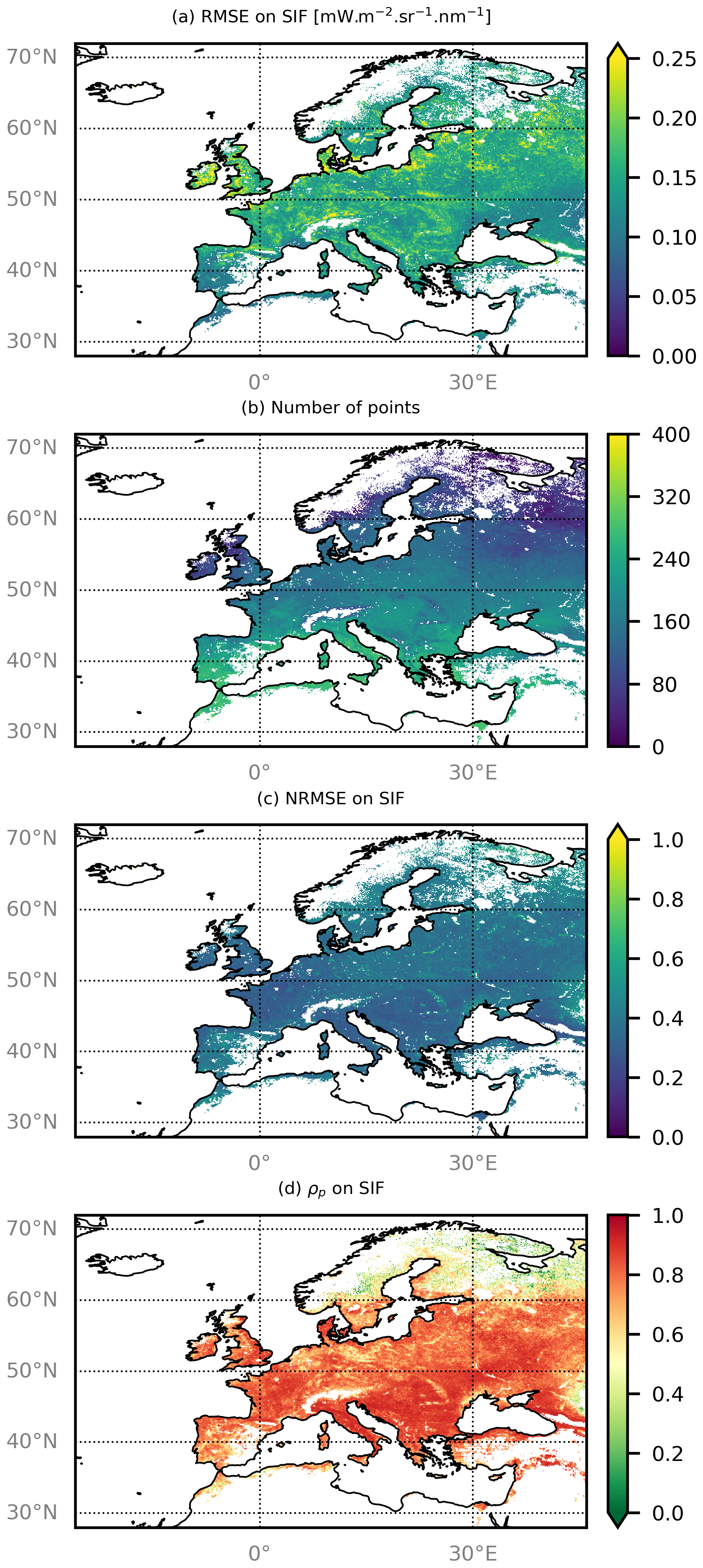
Figure 4 Grid-pointwise evaluation of the performance of the match between NN and observations for the test dataset. From top to bottom: the RMSE, the number of comparison per pixels, the NRMSE, and the Pearson correlation. Units are indicated where applicable.

Based on the spatial distribution of observations over the course of a year, we can expect approximately one observation every 2 d. The RMSE is heterogeneously distributed, highlighting the known areas of C3 crops, and ranges between 0.1 and 0.2 mW m² sr⁻¹ nm⁻¹. The NRMSE distribution is more uniform than the RMSE distribution, averaging at around 20 %. Underestimation appears to be proportional to the values of TROPOMI SIF, so considering a fixed value for the observation error seems inaccurate. That is why, we tested different observation errors.

4.2 Assimilation in the Ebro basin

In the first phase, the NN was trained across the entire European domain. In this section, the saved weights of the neural network are implemented in the assimilation scheme as an observation operator for the SIF. The LAI is simulated and the results are used as input data. In this case, the NN is only used in forward mode, so the weights will not change. Since the observation operator only considers the LAI among the control variables, the accuracy of the LAI representation is the main criterion for evaluating the assimilation results. All assimilation experiments are restricted to the Ebro basin domain.

The LAI increments are substantial on the full Ebro basin domain, reaching up to 0.2 m² m⁻², as shown by the monthly-averaged maps over the C3 crops (Fig. 5). The residuals, the remaining differences between the analysed SIF and the observed SIF, are smaller than the innovation vectors, the difference between modeled SIF and observed SIF. This illustrates that the assimilation of SIF leads to the identification of such observed agricultural practices in the model, even when they are not simulated. Here, we observe a confined area around the Ebro basin where LAI increased during the summer of 2021. This pattern was also evident in the other years of the experiment. This confined area is artificially irrigated (Ricart et al., 2016). Irrigation sustains the LAI and SIF, while other areas become drier. This illustrates that the assimilation of SIF leads to the identification of such observed agricultural practices in the model, even when they are not simulated.

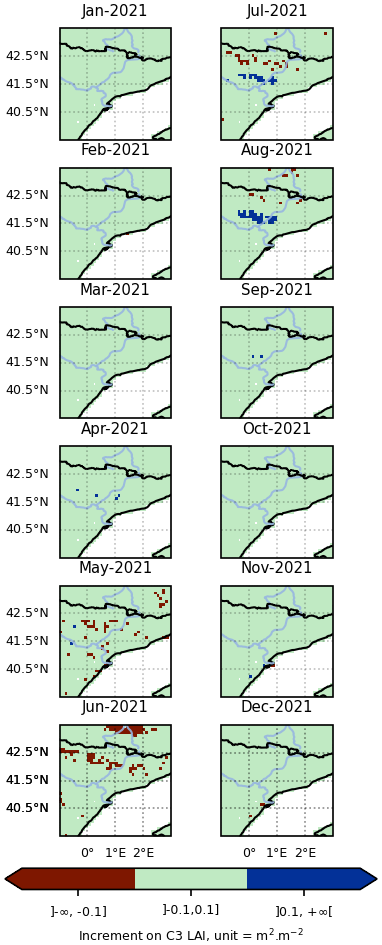
Figure 5 Mean monthly analysis increments of the SIF₂₀ experiment on the LAI of C3 crops over the Ebro domain due to SIF assimilation during the year 2021. Grid cells displaying less than 10 % C3 crops are masked.

This positively impacts on the representation of LAI, as demonstrated by the map of the differences between the RMSEs in Fig. 6a, b, c. During the same period, we calculated the difference in correlation with respect to the 10 d LAI-V1 product between the open-loop experiment and the analysis. The resulting map is displayed in Fig. 6d, e, f. As only one observation is available every 10 d for calculating the correlation, all cells with a F-test p-value higher than 0.01 were removed. This ensures that significant correlation and RMSE values are displayed. This mask is used for the RMSE displayed in Fig. 6a, b, c and the correlation panels displayed in Fig. 6d, e, f. Figure 6a, d show the results averaged over the first full year of TROPOMI SIF assimilation. Due to the small number of days on which both the 10 d LAI-V1 observation (with no temporal interpolation) and TROPOMI SIF were available, many grid cells were discarded by the F-test. An extensive decrease in RMSE is observed for the remaining grid cells, except in some areas of the French Pyrenees. The improvement in correlation is more heterogeneous, with more areas showing a loss of correlation or no change. The results obtained during the second year of assimilation, displayed in Fig. 6b–e, cover a larger area and confirm the results of the first year. Overall, the RMSE decreased except in some specific areas, while the correlation with respect to LAI observations was only around the Ebro river basin. Once the results from both years are combined, Fig. 6c, f provides a clearer picture of the improvements brought about by the assimilation of TROPOMI SIF. Overall, the RMSE decreased except in some areas of the Pyrenees mountains, and the correlation increased over the crop areas of the Ebro basin, as shown in Fig. 1c, but not in forest and bare soil areas. There were no significant discrepancies between the results of the first and second years of assimilation. Furthermore, a greater number of grid cells passed the F-test in the second year, confirming that the first year of assimilation matching the year of the data used to train the observation operator is not problematic.

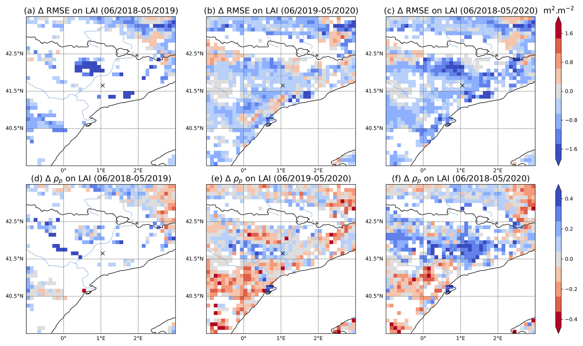
Figure 6 Differences (SIF₂₀-OL) over the Ebro domain in (a, b, c) RMSE and in (d, e, f) ρ_p computed with respect to LAI observations after and before assimilation of SIF averaged from: June 2018 to May 2019 (a–d); from June 2019 to May 2020 (b–e) and from June 2018 to May 2020 (c–f).

For the irrigated pixels marked with a cross in Fig. 6, the SIF and LAI estimates from the analysis are closer to the observed values in terms of RMSE and correlation. This is evident in the time series of both OL and SIF₂₀, which are displayed in Fig. 7 and were extracted over this specific irrigated grid cell. The LAI and TROPOMI SIF observations displayed in Fig. 7 all show regrowth of the vegetation in late summer each year, which is not seen by the OL experiment. However, assimilation of TROPOMI SIF (i.e. the SIF₂₀ analysis results shown in Fig. 7) tends to be more accurate. There has been an improvement in terms of the agreement between TROPOMI SIF and LAI. The SIF estimated from the analysis remains smaller than the observed TROPOMI SIF, but captures the temporal trends. As the estimated SIF does not necessarily represent the true SIF, but only the aggregated TROPOMI SIF measurements used, we cannot comment on the physicality of this underestimation in our SIF representation. As highlighted in Sect. S2 of the Supplement, the neural network is not a substitute for a SIF physical model, as demonstrated by the comparison with airborne measurements of SIF over the same area from the HyPLant campaign (Rascher et al., 2015).

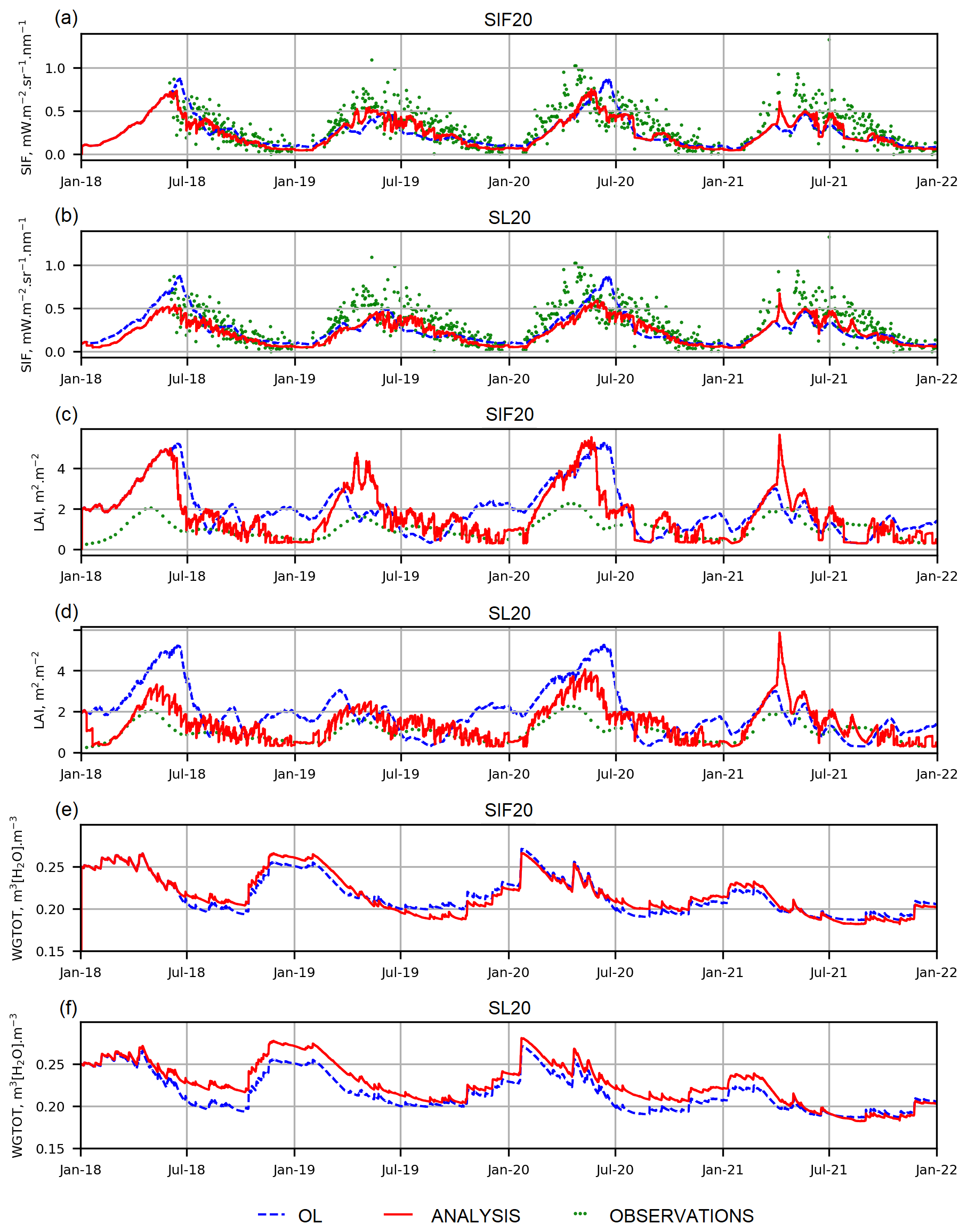
Figure 7 Timeseries extract on the cell locate in 1.05° E, 41.65° N for the SIF (a, b), the LAI (c, d) and the the total soil moisture (WGTOT) in the column (e, f). The open loop (OL in Table 1) indicated with dashed blue lines, SIF₂₀ (a, c, e) and SL₂₀ (b, d, f) analyses with the plain red line in their respective panels and observations with green dots. The observations for the SIF, and LAI are respectively extracted from TROPOMI SIF and LAI-300 described in Sect. 2.2.3.

Assimilating SIF improves the correlation with FLUXCOM-GPP over the full Ebro domain, as shown in the boxplots in Fig. 8. This demonstrates that, on average, the SIF₂₀ experiment provides an equally accurate representation of GPP as the LAI₂₀ experiment, and a more accurate representation than the OL experiment. Regarding LAI, Fig. 9 shows that SIF₂₀ provides a better RMSE than the OL experiment, as indicated by Fig. 6, but this RMSE remains slightly higher on average than the LAI₂₀ experiment over the Ebro domain.

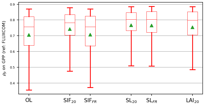
Figure 8 Box plot of the correlation between analysis, open-loop simulated GPP and the FLUXCOM dataset over the Ebro domain. From left to right: Open-loop, SIF₂₀, SIF_FR, Coassimilation SL₂₀ and SL_FR configurations and assimilation of LAI-V1. The boxes represent the 25th and the 75th percentiles, the whiskers the 5th and 95th percentiles. The red line represents the 50th percentile and the green triangle the mean.

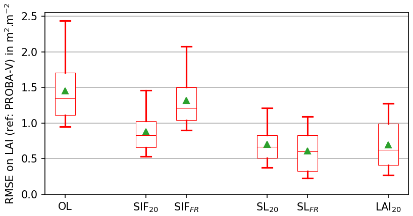
Figure 9 Boxplot of the RMSE for the different LAI predictions taken between June 2018 and June 2020 over the Ebro domain. Box represents the 25th and the 75th percentiles, the whiskers the 5th and 95th percentiles. The red line represents the 50th percentile and the green triangle the mean.

In addition to the experiment with 20 % (SIF₂₀), we also tested assimilation with two different error scenarios, namely SIF₀₁ and SIF_FR, which is a combination of the two first scenarios.

The time series displayed in Fig. 10 are showing the differences between the Ebro domain averaged RMSE with respect to LAI-V1 10 d observations from the different analyses and the one from the open-loop RMSE. The RMSE for SIF₂₀ analysis tends to match the RMSE from the reference LAI₂₀ experiment and is sometimes even lower. In the case of SIF₀₁ and SIF_FR, the RMSE is close to that of the open-loop experiment, even though the SIF_FR configuration provide a better RMSE on LAI than the SIF₀₁ configuration. This suggests that our first guess (i.e. 20 % of relative error) in terms of observation error is close to the optimal situation for minimising the RMSE, and that higher values tend to render assimilation ineffective. For the SIF_FR, this skill loss is also visible in terms of correlation with FLUXCOM GPP according to Fig. 8. Experiment SIF₂₀ and LAI₂₀ achieve similar accuracy in terms of representation of LAI and GPP, yet SIF₂₀ performances have more variances, but led to five time more observation to be assimilated.

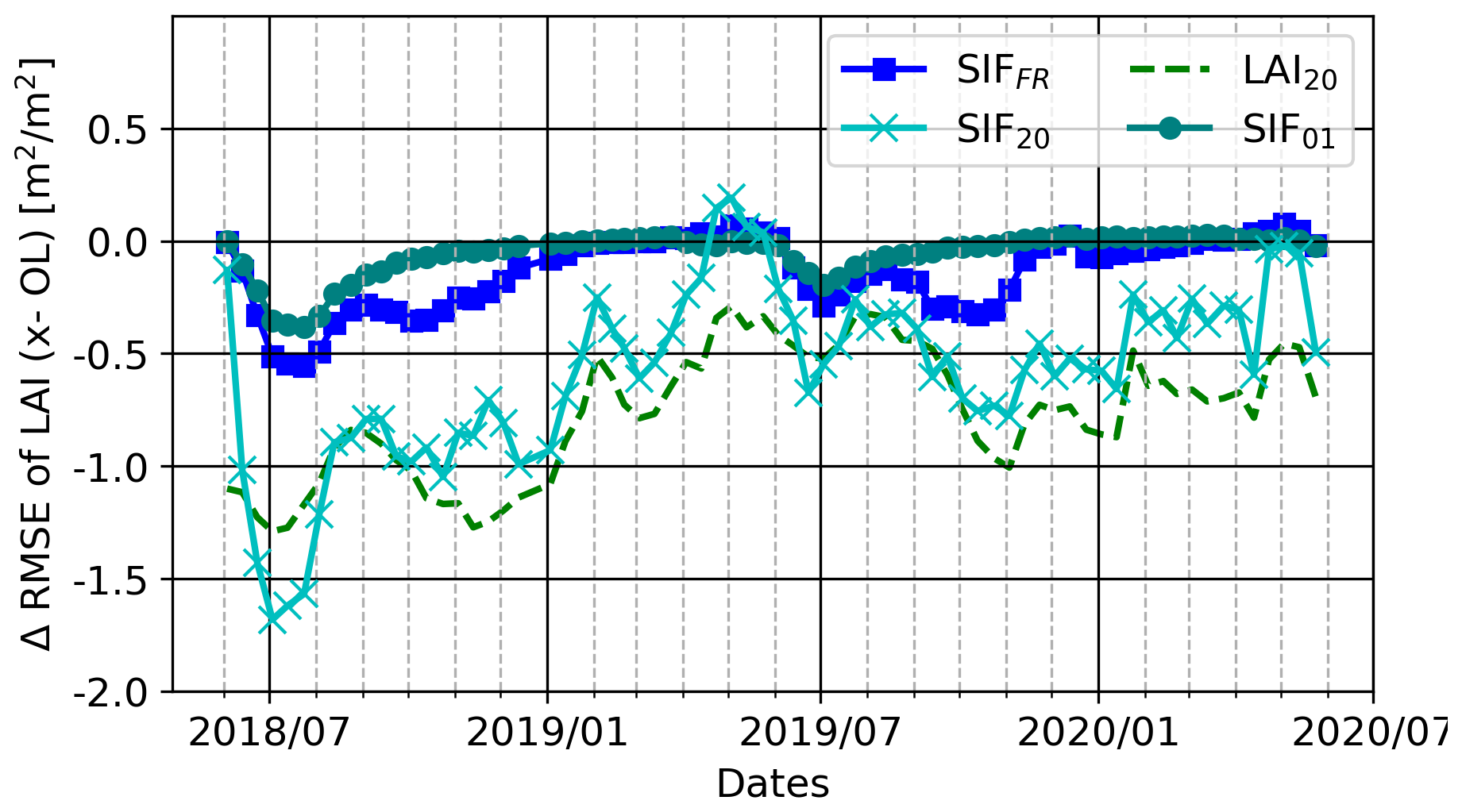
Figure 10 ΔRMSE between the Open-Loop and the LAI analysis of the assimilation experiments from January 2018 to January 2020 over the Ebro domain.

5 Discussion

5.1 Is the Co-assimilation of LAI and SIF provide better results than assimilating one of the two?

When it comes to data assimilation, the question of redundancy in observations is important, since disagreement between observations can degrade the analysis, while agreement can improve it further. Two configurations of co-assimilation, SL₂₀ and SL_FR of the LAI-300 from CLMS and the TROPOMI SIF are run on the Ebro basin domain. We compare the RMSE on LAI for each cell of the assimilation domain averaged from June 2018 to May 2020 for all assimilation experiments and display the results in Fig. 9. This co-assimilation configuration achieves an RMSE on LAI that is at least as good as that achieved by assimilating LAI or SIF alone and highlights some synergistic behaviour in the assimilation of both observations. This result is also evident in the correlation with FLUXCOM GPP, as shown in Fig. 8. In terms of local behaviour, comparing the SL20 time series with the SIF₂₀ time series in Fig. 7 shows that co-assimilation leads to much better agreement with observed LAI while keeping SIF close to TROPOMI SIF. This is especially true during spring where the assimilation of SIF alone led to too high LAI. The SL20 analysis improves also the representation of the second SIF and LAI peak due to irrigation in summer 2020.

While assimilating TROPOMI SIF as the only observation should achieve results similar to the LAI₂₀ experiment with a relative error of 20 %, both cases of co-assimilation (co-assimilating SIF alongside LAI) achieve better results than assimilating only LAI-V1 or TROPOMI SIF, regardless of the observation error on TROPOMI SIF. Furthermore, the FR configuration in co-assimilation does not degrade the results as much as when only TROPOMI SIF is assimilated, providing a more consistent improvement than the SL₂₀ analysis. This demonstrates that co-assimilation of TROPOMI SIF with a 10 d LAI product improves the LAI representation further. The key is that the assimilation of TROPOMI SIF leads to changes in day-to-day monitoring of fluxes and LAI, albeit with some variance. In contrast, the assimilation of unbiased LAI reduces variability around LAI observations. This results in more accurate trends and better agreement with LAI observations and, to a lesser extent, GPP observations than the assimilation of the LAI product alone, as illustrated in Fig. 8.

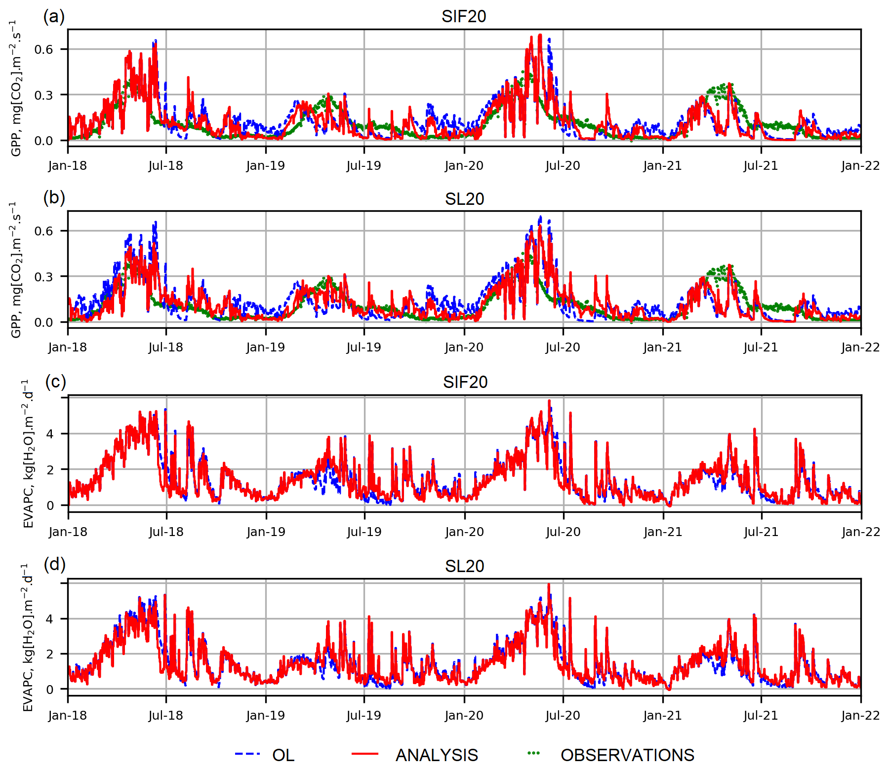
Figure 11 Same as for Fig. 7 but for the daily mean GPP (a, b) and the daily cumulated evapotranspiration (EVAPC) in panels (c, d). The open loop (OL in Table 1) indicated with dashed blue lines, SIF₂₀ (a, c) and SL₂₀ (b, d) analyses with the plain red line in their respective panels and observations with green dots. The observation of GPP are extracted from FLUXCOM database.

5.2 Does the GPP require additional observations to be better constrained?

Unexpectedly, the GPP seems to benefit less from TROPOMI SIF assimilation, even though SIF is known to be well correlated with the GPP. While the GPP is improved on average across the domain by assimilating TROPOMI SIF, the local comparison displayed in Fig. 7 shows that it is difficult to substantially improve the analysed GPP. It is slightly better in case of coassimilation without solving the inaccuracy in the GPP representation. This result stems from the way the GPP is modelled by the ISBA LSM. The modelled GPP depends not only on the vegetation parameter, but also on the soil water content. Assimilating SIF often results in a more accurate representation of LAI, and in our local case, it adds more LAI in summer than the open-loop model forecasts. This increase in LAI causes the model soil to dry out, as shown by the total soil moisture (WGTOT) in the soil column in Figs. 7, 11, and increases the evapotranspiration accumulated over the day (EVAPC in Fig. 11). Consequently, the computed GPP cannot increase, whereas the observed counterpart (i.e. FLUXCOM) captures this second increase in late summer. FLUXCOM is an observation product based mainly on atmospheric variables, but it also incorporates vegetation and temperature data from MODIS satellites. This remote sensing data helps FLUXCOM to identify these recurrent increases in GPP due to artificial irrigation (see figures in the Supplement, Sect. S3). Assimilating SIF yields the same results as assimilating LAI directly from the GPP perspective. As such, assimilating SIF corrects the LAI and updates the soil water content to balance the change in LAI. However, it cannot infer an increase in soil water content, which would make the model's GPP more similar to the FLUXCOM estimate.

6 Conclusion

In this article, we examined the use of a deep learning emulator of TROPOMI SIF as an observation operator, and explored the advantages of incorporating TROPOMI SIF into a land surface model with this observation operator. The neural network operator takes the LAI and three metadata as inputs: the two geographical coordinates and the day of the year. Using this simple setup, we achieved an average RMSE of 0.15 mW m² sr⁻¹ nm⁻¹ on the TROPOMI SIF averaged estimate, with no evident overfitting. The Pearson correlation coefficient between the neural network estimate and TROPOSIF is greater than 0.8, with higher correlations observed in cropland areas than in coniferous areas. However, the neural network struggles with statistically extreme values, which increases the averaged RMSE and introduces bias. It is also unable to capture small variations close to the expected mean value. Nevertheless, it does capture major changes in the TROPOMI SIF, such as those due to the changing seasons.

The neural network was then successfully employed as an observation operator, taking into account the observation error relative to the average TROPOMI SIF value. Several assimilation experiments were conducted over an irrigated cropland area in the Ebro basin. TROPOMI SIF assimilation had a similarly positive impact on LAI as assimilation of the 10 d LAI observation product. However, it should be noted that daily assimilation of TROPOMI SIF yields a higher update rate than assimilation of 10 d LAI observations. Despite not being predicted by the LSM or provided as inputs to the neural network, irrigated areas were well represented. The analysis also improved the representation of both TROPOMI SIF and changes in GPP, which are both important for monitoring the carbon cycle.

This study has shown that, when assimilating SIF alone, an observation error of 20 % leads to the best assimilation performance. In a co-assimilation framework incorporating LAI, the representation of vegetation variables (i.e. LAI and GPP) improves further, demonstrating the value of redundancy in observations used in a data assimilation system. However, the best performance is obtained using a more complex error description (FR). Further research is required to quantify observation errors accurately. Unlike the assimilation of LAI, assimilation of TROPOMI SIF leads to a small improvement in GPP representation over unmodelled irrigated areas, since additional water supply is not represented.

We demonstrated the advantages of integrating TROPOMI SIF products into a land data assimilation system by applying a deep learning operator. This opens up new possibilities for assimilating new SIF products. Although the neural network operator was designed for TROPOMI SIF products, it can be adapted for other SIF products. We also addressed the co-assimilation of SIF with LAI, a process that could be extended to other satellite products, such as land surface temperature.