Towards constraining the drivers of variability and trends in subantarctic productivity

The subantarctic Southern Ocean is a climatically important region, where primary production largely drives the seasonal uptake of atmospheric CO₂, contributing to the sequestration of anthropogenic carbon emissions. Seasonal iron and light limitation control annual net primary production (NPP) in this region, but the explicit mechanisms that drive differences in NPP between years (NPP interannual variability) remain elusive due to sparse observations. This uncertainty is reflected in inconsistent interannual variability and trend estimates of remotely-sensed NPP algorithms. Without clear mechanistic underpinning, confidence in remotely-sensed NPP trends remains low and hinders predictive capability. To overcome observational limitations and better understand the drivers of interannual NPP variability, we analysed the explicit bottom-up and top-down controls of depth integrated NPP in a biogeochemical ocean model historical run (PISCES-QUOTA-FE; 1958–2022) in the subantarctic zone south of Tasmania, Australia. The highest NPP years were primarily driven by increased relief of iron limitation, with iron supplied from both deeper mixing in winter/spring and enhanced remineralisation in summer. In spring, higher phytoplankton growth rates were decoupled from surface biomass, such that years with higher NPP were due to faster growth in the mixed layer. Faster growth rates emerged following deeper winter mixed layers, driving phytoplankton distributions deeper in winter and reducing mixed layer grazing loss rates in spring. This generated a predator-prey dynamic favouring surface biomass accumulation moving into summer. Thus, inconsistent remote-sensing NPP estimates may derive from how algorithms link biomass (rather than growth rates) to NPP. We applied our analysis to a subset of CMIP6 models, and while all historical simulations converged with respect to positive trends in NPP, bias from sea surface temperature trends influenced the mechanisms driving interannual NPP variability. These findings show that interacting top-down and bottom-up processes can decouple changes in NPP with respect to phytoplankton biomass, which has important implications for remote sensing NPP estimates based on biomass. Therefore, the need for cautionary approaches to NPP trend interpretation is highlighted. Additionally, further observational data, including zooplankton grazing and phytoplankton biomass distributions over depth are needed to ground truth mechanistic understanding of NPP drivers and develop models through mechanistic inclusion.

1 Introduction

The subantarctic region south of Australia hosts the seasonal formation of subantarctic mode water which transports heat, carbon and nutrients below the pycnocline and into the low latitude ocean (Sabine et al., 2004; Khatiwala et al., 2013). Over the annual cycle, this region is a net CO₂ sink (Lenton et al., 2013; Shadwick et al., 2023), driven predominantly by biological processes (primary production) (Shadwick et al., 2015; Yang et al., 2024a). However, the impact of warming, freshening, stratification and acidification (Orr et al., 2005; Keeling et al., 2010; Bindoff and Hobbs, 2013; Pardo et al., 2017; Auger et al., 2021; Thomalla et al., 2023) due to the uptake of excess anthropogenic heat and carbon dioxide (Feely et al., 2004; Cheng et al., 2022) could alter this region's role in global carbon cycling. How primary productivity responds to these changes is uncertain but is critical to assessing how regional biogeochemical cycles and ecosystems change (Deppeler and Davidson, 2017; Henley et al., 2020; Anugerahanti and Tagliabue, 2024; Henson et al., 2024; Hutchins and Tagliabue, 2024).

While remote sensing has begun to reveal regional trends in Southern Ocean net primary production (NPP) a deeper understanding of the underlying mechanisms is needed. Trends in NPP from different satellite estimates show varied relationships to plausible physical drivers including sea surface temperature (SST) and mixed layer depth (MLD) (Ryan-Keogh et al., 2025b), reducing confidence in our understanding of the why NPP is changing (Tagliabue et al., 2021). Much of this uncertainty stems from the mechanistic parameterisation of NPP across satellite algorithms, which is derived from different estimates of the depth inventory of phytoplankton, biomass and the rate at which they divide. Each variable used to derive NPP, including SST, absorption coefficients, the chlorophyll to backscatter ratio, nutrient concentrations, photosynthetically available radiation and MLD, can in turn carry its own form of bias (Ryan-Keogh et al., 2023a).

Significant advances in our understanding of the drivers of seasonal and interannual variability in biogeochemistry in the Subantarctic Zone (SAZ) have been achieved using observations generated by Southern Ocean Time Series (SOTS) program, located south-west of Tasmania, Australia (Wynn-Edwards et al., 2020; Shadwick et al., 2023; Yang et al., 2024a; Shadwick et al., 2025; Traill et al., 2025). In this region, iron has been shown to be a seasonally limiting factor for primary productivity using both composite time series observations and optical methods (Schallenberg et al., 2020; Traill et al., 2025). The strong link between seasonal and sub-seasonal iron supply and NPP in the SAZ (Bowie et al., 2009; Barrett et al., 2021; Traill et al., 2024, 2025) may be in part driven by variability in the southern extension of the East Australian Current (Traill et al., 2025), which moves southward into the SOTS region through summer (Yang et al., 2024a; Traill et al., 2025). However, the decoupling of iron distributions from the prevailing physical supply pathways due to biological processes, including uptake and remineralisation (Tagliabue et al., 2012; Traill et al., 2024, 2025), and absence of high resolution multi-year iron and primary production incubation measurements, challenges our understanding of NPP drivers using observational methods.

Biogeochemical models are a valuable tool in addressing this research gap. By assessing the mechanistic links between environmental drivers and productivity, models can help us to investigate the explicit links between micronutrient supply and productivity over broad temporal and spatial scales. Recent improvements in the numerical modelling of iron biogeochemical cycling have improved the ability of models to recreate observed dissolved iron (DFe) distributions (Tagliabue et al., 2023), a key step in assessing NPP drivers in the iron limited Southern Ocean. In CMIP6 models, projected increases in Southern Ocean NPP are fairly consistent (Kwiatkowski et al., 2020; Tagliabue et al., 2021; Fisher et al., 2025). However, without a mechanistically constrained observational understanding of emerging trends it is impossible to know if models are recreating these trends for the right reasons (Laufkötter et al., 2015; Tagliabue et al., 2021; Fisher et al., 2025; Ryan-Keogh et al., 2025b). This leaves future projections highly vulnerable to uncertainties in the physical response of the ocean to a changing climate. Amidst this uncertainty, the first step is to determine exactly what is driving trends in the models (Tagliabue et al., 2021; Fisher et al., 2025).

In this paper, we examine the drivers of interannual productivity in the SAZ south of Australia using a combination of observational and biogeochemical model analyses. Firstly, we aimed to determine the relationship between interannual productivity variability and broadscale drivers from observational NPP data streams, specifically probing the influence of the subtropical front (STF) as a proxy for the extension of the East Australian Current (EAC) into the region. Secondly, using a biogeochemical model, we aimed to determine the explicit mechanisms by which physical drivers influence phytoplankton growth and loss rates and ultimately NPP changes by interrogating the explicit nutrient limitation, temperature limitation, light limitation and grazing terms. Finally, we aim to determine the variability in drivers of productivity across a suite of CMIP6 models, and discuss the implications of these findings for NPP trends, helping to disentangle uncertainty in first-order productivity drivers and observational/model disagreement.

2 Methods

2.1 Study region and oceanographic properties

To investigate the mechanisms driving interannual variability in NPP, the region 45–49° S, 140–150° E was selected (Fig. 1a) and referred to as the study region hereafter. In assessing temporal variability and trends in the SOTS region, all observational and simulated terms have been grid cell area weighted and spatially averaged over the SOTS region. This regional subset, slightly larger than the region previously defined around the SOTS observatory (140–144° E, 46–48° S; e.g. Yang et al., 2024a), was selected to capture the broader seasonal and interannual variability in STF movement that might be associated with the East Australian Current extension (Fig. 1a) and larger scale NPP. The larger spatial average also helps remove higher frequency variability and facilitate the identification of small but emerging temporal trends.

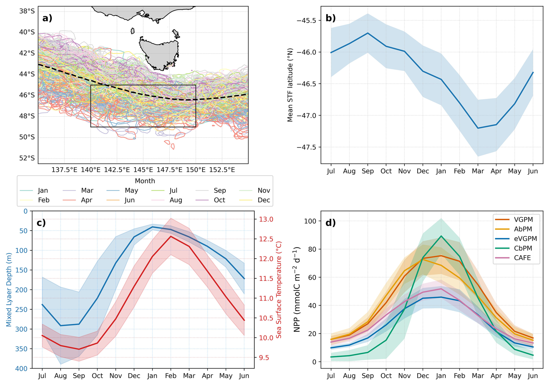
Figure 1 Regional bounding box (solid black line) in which observational and modelled climatological averages were calculated. Mean monthly contours of the subtropical front (STF; 11° isotherm at 100 m depth, definition per Orsi et al. 1995) for the period 1998–2022 are given by coloured lines, with the mean given by the dashed black line. (b) Climatological STF extent (1998-2022) as the mean latitude (° N) (±1σ from the mean) of the 11° isotherm at 100 m depth (Orsi et al., 1995). (c) Climatological (1998–2022) means of MLD (blue) derived from Hadley EN4.2.2. profiles and SST (red) from ARMOR-3D, shading is ±1σ from the mean in the SOTS region box (a). (d) Climatological mean NPP estimates from OC-CCI based satellite algorithms (1998–2022), shading is ±1σ from the temporal mean.

The SOTS observatory, nominally located at 142° E, 47° S, is situated in the SAZ, is considered broadly representative of SAZ waters south of Australia between 90–145 ° E (Trull et al., 2001; Shadwick et al., 2015; Yang et al., 2024b). The seasonal oceanographic, biogeochemical and productivity cycles in the SOTS region are well described (Shadwick et al., 2015, 2025; Eriksen et al., 2018; Schallenberg et al., 2019; Trull et al., 2019; Traill et al., 2025). The SOTS region is influenced by contrasting physical properties north and south of the STF. Warm, salty subtropical waters from the Zeehan and East Australian Current extensions are present in the surface. These overlay cooler, fresher and well oxygenated subantarctic mode waters formed during winter where mixed layer depths can exceed 300 m (Fig. 1c). The seasonal progression of the STF reaches its maximum climatological southern extent in March, slightly later that peak climatological SST in February (Fig. 1b, c). Climatological NPP increases rapidly through spring as the mixed layer shoals, peaking in December through to February (Fig. 1d).

2.2 Observational datasets

Remote sensing time series data for the period 1998–2022 were compiled to assess variability and trends in physical drivers (SST, MLD and STF locations) and NPP (Fig. 1). Physical environmental variables SST and STF were derived from the Copernicus Marine Service Multi Observation Global Ocean ARMOR-3D L4 analysis product (Table 1). This observation-based product combines in situ temperature and salinity profiles (predominantly Argo network) with synthetic satellite sea surface temperature and altimetry derived salinity fields using an optimal interpolation method (Guinehut et al., 2012). For MLD, the same product as used in the generation of the OC-CCI NPP algorithms was selected (Ryan-Keogh et al., 2023a). MLDs were derived from the Hadley EN4.2.2 temperature and salinity profiles (Good et al., 2013) and the Gouretski and Reseghetti (2010) bias corrections, using a density threshold of 0.03 kg m⁻³ (De Boyer Montégut et al., 2004).

Table 1 Catalogue of remote sensing observations, model output and diagnostics. For phytoplankton class specific variables, i denotes individual phytoplankton classes (i= Nanophytoplankton, Picophytoplankton, Diatoms). References are provided for specific data sources, with methods used to determine specific metrics given in parenthesis. For PISCES-Quota-Fe, references given are for the output configuration used in this study, with those in parentheses denoting specific equations used to generate terms. If no method is given, variable equations are provided in the model description references. Except where otherwise stated, PISCES-Quota-Fe variable depth integrals were calculated over the full depth grid.

Table 2 Continued.

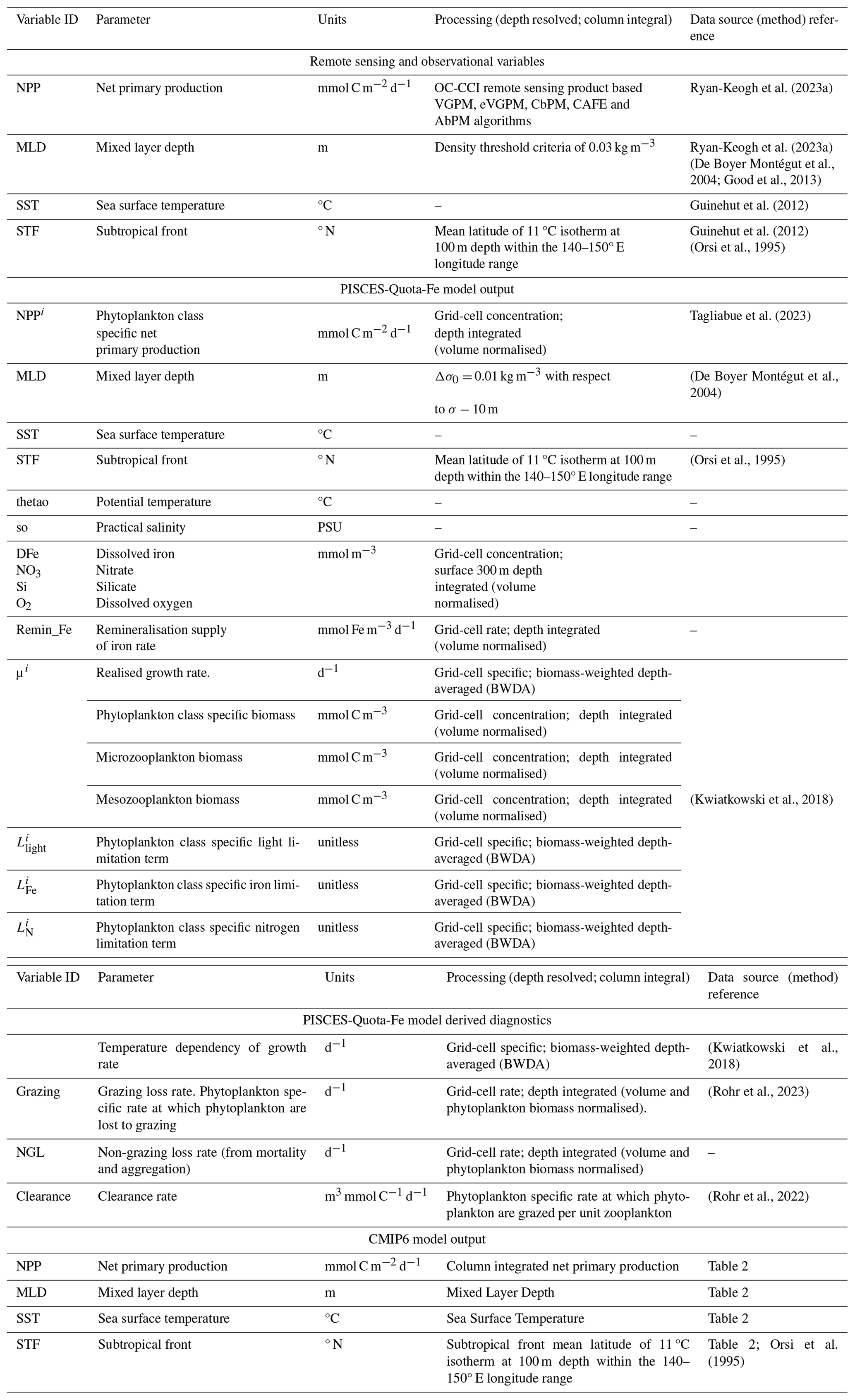
Estimates of NPP from five remote sensing algorithms were obtained from the OC-CCI-based dataset processed by Ryan-Keogh et al. (2023a): the Vertical Generalized Production Model (VGPM; Behrenfeld and Falkowski, 1997), the Eppley-VGPM which includes the Eppley temperature dependent growth parameterisation (eVGPM; Eppley, 1972), the Carbon-based Production Model (CbPM; Westberry et al., 2008), Carbon, Absorption, and Fluorescence Euphotic-resolving model (CAFE; Silsbe et al., 2016), and Absorption-based Production Model (AbPM; Lee et al., 2011). Detailed discussion on the algorithm input dependencies and assessment is given in Fig. 2 and Ryan-Keogh et al. (2023a, 2025b).

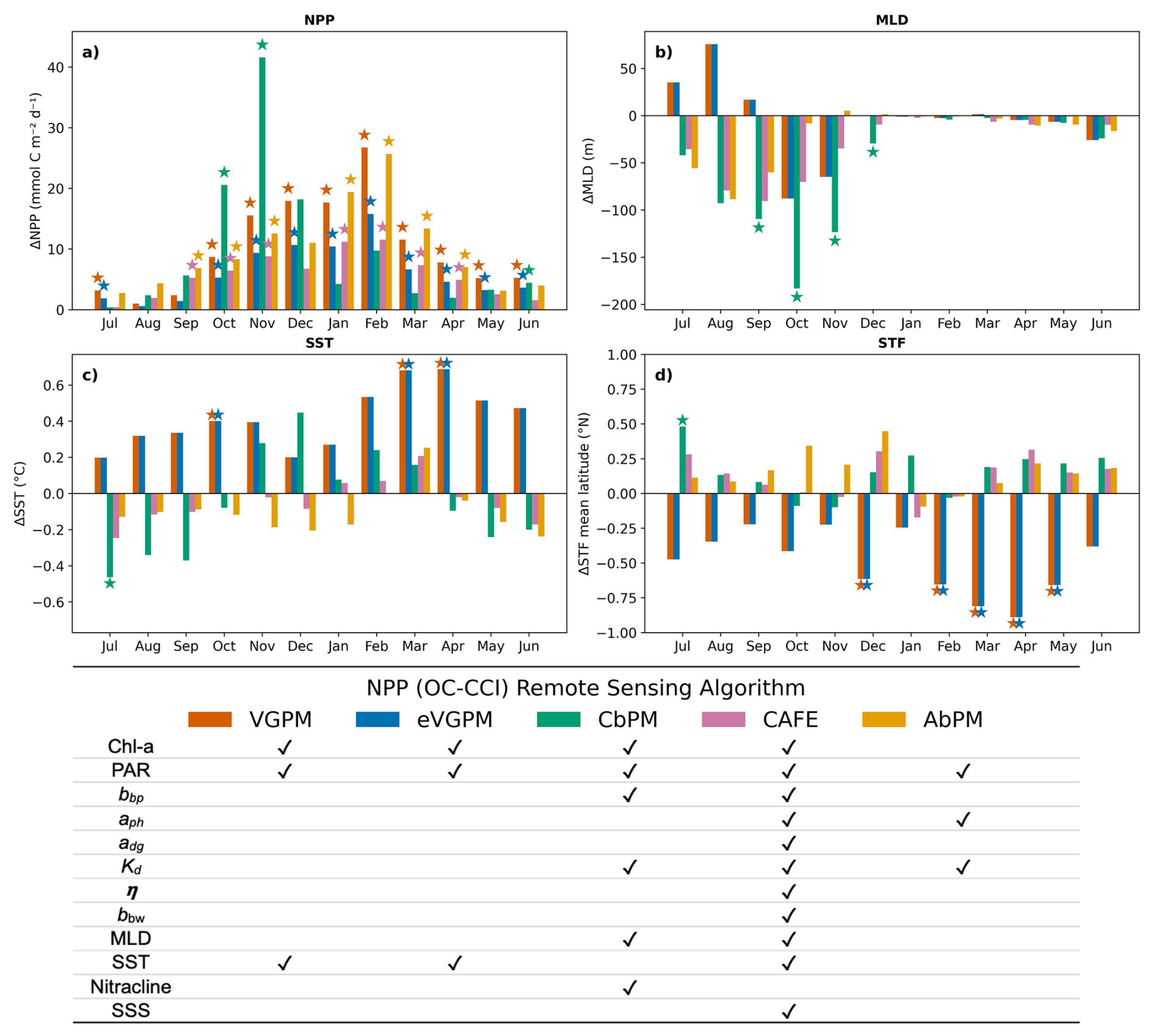
Figure 2 (a) Change in integrated NPP (ΔNPP) from five OC-CCI-based remote sensing algorithms calculated from the difference in climatological means of the five highest and five lowest NPP seasons for observations in the region 140–150° E, 45–49° S, for the period 1998–2022. Corresponding changes in the physical drivers for corresponding algorithm high and low NPP year groups are shown for (b) ΔMLD, (c) ΔSST and (d) ΔSTF mean latitude. Positive values of ΔMLD, ΔSST and ΔSTF indicate deeper MLDs, warmer SSTs and further north mean STF latitude during high NPP seasons respectively. Stars indicate that mean monthly climatological difference in the selected high and low NPP season groups is significant relative to the full time series climatological variability at the p<0.05 level (10 000 iteration random year bootstrapping analysis). The figure legend describes the specific observational and spectral variables used in each NPP algorithm (Chlorophyll a (Chl-a), photosynthetically active radiation (PAR), backscatter at 443 nm (b_bp), phytoplankton absorption at 443 nm (a_ph), detrital absorption at 443 nm (a_dg), diffuse attenuation coefficient at 490 nm (K_d), the spectral slope of backscatter (η), the backscatter of pure water (b_bw), Hadley EN4.2.2 mixed-layer depth (MLD), sea surface temperature (SST), nitracline depth, and sea surface salinity (SSS)).

2.3 Resolving the mechanisms driving net primary production interannual variability in PISCES-Quota-Fe

To understand the mechanisms between physical and biogeochemical drivers of interannual variability in NPP and move beyond the limitations imposed by observational platforms, we use an ocean b]iogeochemical model. This approach allows us to dissect the explicit thermal, light, nutrient and loss processes driving interannual variability in NPP explicitly (Table 1).

We analyse output from the Pelagic Interactions Scheme for Carbon and Ecosystem Studies Quota biogeochemical model with improved iron cycling (PISCES-Quota-Fe) (Tagliabue et al., 2023). PISCES-Quota-Fe is built upon PISCES-Quota (Kwiatkowski et al., 2018) and incorporates three phytoplankton types (nanophytoplankton, picophytoplankton and diatoms), independent carbon, nitrogen, phosphorus, silica and iron stoichiometry within phytoplankton, and dissolved organic and particle pools. Two zooplankton groups (microzooplankton and mesozooplankton) are included, but both have fixed stoichiometry (Kwiatkowski et al., 2018). PISCES-Quota-Fe also includes two aeolian-derived lithogenic particle tracers (fine lithogenic particles and aggregated lithogenic particles), two additional particulate authigenic iron tracers (small and large particulate authigenic Fe), an updated Fe chemistry routine that decouples the cycling of colloidal iron from the equilibrium with ligands previously employed in PISCES-Quota, and updated ligand parameterisation based on optimised model-observation fit (Tagliabue et al., 2023).

These changes to the iron cycling in PISCES-Quota-Fe result in improved skill over PISCES-Quota relative to global DFe and PFe observations, while retaining performance in core biogeochemical tracer distributions (nutrients, chlorophyll, oxygen, carbon export) (Tagliabue et al., 2023). These improvements are particularly relevant to the Southern Ocean iron cycle, where interchange between particulate iron pools controls the resupply of sub-surface iron sources that can impact seasonal resupply during winter mixing (Bressac et al., 2019; Tagliabue et al., 2019, 2023). A full description of the model including equations and comparison between PISCES-Quota and PISCES-Quota-Fe are described in Tagliabue et al. (2023).

PISCES-Quota-Fe was coupled to the Nucleus for European Modelling of the Ocean version 4.0 (NEMO-v4.0) general ocean circulation model and Sea Ice modelling Integrated Initiative (SI3) sea ice model. The hindcast simulation was forced with JRA-55 atmospheric reanalysis (Tsujino et al., 2018) for the period 1958–2022. Horizontal model resolution is nominally 2° but increases to ∼1° at high latitudes and ∼0.5° at the equator, while the vertical resolution varies between 10 and 500 m thickness over 31 depth-coordinate levels. Model output analysis was performed on the mean monthly time series from 1975–2022 to avoid model initialization bias in the first 17 years of the simulation (Buchanan and Tagliabue, 2021). The analysis presented here was restricted to the observational study region in Fig. 1a. Key model output and diagnostics are described in Table 1.

2.4 Analysis of productivity drivers, mechanisms and responses

To determine the relative influence of mechanisms (Table 1) driving interannual variability in primary productivity across both observational and simulated data, we considered the highest and lowest NPP periods in respective time series. This was done to assess the highest anomalous NPP years and identify the most important drivers, since competing drivers and their interactions across the whole time series limits correlative signals across the whole time series. We first selected the 5 highest and 5 lowest seasons (Austral summer; July to June) of integrated NPP from the time series. The selection of 5 highest/lowest NPP years was based on the top and bottom 10 % percentiles of the 48-year simulated time series, where the top 5 years of seasonally integrated NPP values lie outside 1 standard deviation from the mean. We also used the top/bottom 5 years in observational time series, noting the limitation of a shorter observational time series with which to compare.

The differences in each variable (var) between years corresponding to the highest and lowest NPP were calculated for all variables and assigned the Δ prefix (Eq. 1).

$$\begin{array}{}\text{(1)}& \mathrm{\Delta }\mathrm{var}\left(m\right)={\overline{\mathrm{var}}}_{\mathrm{high}}\left(m\right)-{\overline{\mathrm{var}}}_{\mathrm{low}}\left(m\right)\end{array}$$

Where Δvar (m) is the difference in mean monthly climatological values for variable var in month m between the high- and low-NPP years, ${\overline{\mathrm{var}}}_{\mathrm{high}}\left(m\right)$ is the mean monthly climatological value of var at month m calculated over the five highest integrated NPP years, and ${\overline{\mathrm{var}}}_{\mathrm{low}}\left(m\right)$ is the mean monthly climatological value of var at month m calculated over the five lowest-NPP years.

To assess whether the differences between high- and low-NPP years (Δ-variable) were statistically significant relative to background variability, we applied a non-parametric bootstrap resampling approach. This method is well suited to our analysis because it tests the difference between two empirical samples (high- and low-NPP years), rather than comparing a single sample against a theoretical population mean and does not assume underlying distributions. Specifically, we generated an empirical distribution of Δ-variable values by randomly resampling years from the full time series without replacement, repeating this process 10 000 times. This allowed us to calculate two-sided p-values and corresponding 95 % confidence intervals for each variable, representing the probability that the observed Δ-variable could arise by chance under the null hypothesis of no systematic difference. The bootstrap analysis was applied independently to all variables listed in Table 1 across both observational and model-based datasets.

2.5 Productivity projections in CMIP6 models

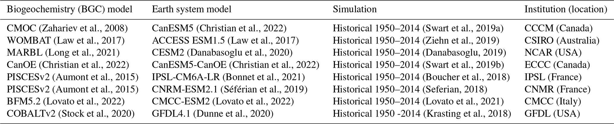
In addition to remote sensing NPP algorithms and PISCES-Quota-Fe, we examined trends in NPP and its drivers across 8 earth system models from the historical Coupled Model Intercomparison Project Phase 6 (CMIP6) simulation suite (Table 2). CMIP6 model output was sourced from the Earth System Grid Federation (Table 2), with model selection restricted to those with outputs saved for gridded temperature at depth in order to derive STF locations (Table 1). Trends in spatial mean monthly NPP, MLD, SST and STF mean latitude anomalies for remote sensing algorithms (1998–2022), PISCES-Quota-Fe (1975–2022) and historical CMIP6 model (1950–2014) were determined using an ordinary least squares linear regression. Environmental variable analysis was performed using the same non-parametric bootstrap resampling method described in Sect. 2.4.

3 Results

3.1 Remote Sensing Products Disagree on the Drivers of Interannual Variability in NPP

When we examined the difference in potential drivers of ΔNPP, calculated as the difference in climatological depth integrated NPP between years corresponding to the highest and lowest periods of total seasonally integrated NPP, inconsistent patterns emerged depending on the NPP algorithm used (Fig. 2). In the first case, ΔNPP in VGPM/eVGPM models was associated with occasionally deeper MLDs, but consistently warmer SSTs and a STF latitude located further south. Alternatively, ΔNPP in CbPM, AbPM, CAFE algorithms were associated with shallower MLDs and insignificant but indicative cooler SSTs and a STF latitude located further north (Fig. 2).

For VGPM/eVGPM algorithms, positive ΔNPP (higher NPP) was associated with significantly higher SSTs in spring (October) and autumn (March–April), coincident with a mean STF latitude located significantly further south through summer and autumn (Fig. 2). Higher NPP in VGPM/eVGPM algorithms co-occurred with deeper MLDs through winter and shallower MLDs in spring (October-November), however the direct association between NPP and MLD not statistically significant (Fig. 2b). The highest ΔNPP was observed in February and was associated with a shallower MLD and a STF latitude further south, indicative of a greater presence of warmer subtropical waters. Increased VGPM/eVGPM ΔNPP at elevated SSTs is not surprising given the temperature dependent growth rate parameterisation of VGPM/EVGPM algorithms. However, MLD is not directly included in these algorithms, so it is interesting to see deeper winter and spring MLDs at elevated SSTs.

For the CbPM algorithm, maximum ΔNPP was larger than all other algorithms and occurred in spring (November), while all other algorithms showed maximum ΔNPP values in February (Fig. 2a). The October and November peaks in CbPM ΔNPP were associated with significantly shallower MLD (Fig. 2a, b), and preceded by significantly cooler SSTs in winter (Fig. 2c). Cooler SSTs were consistent with a STF mean latitude further north but not significantly so (Fig. 2d). Similar relationships were observed in the CAFE and AbPM algorithms, however no environmental features were significantly associated with increased ΔNPP. Interestingly, during peak ΔNPP in February, changes in the environment between high and low NPP seasons in CAFE and AbPM algorithms were barely detected (Fig. 2).

3.2 Simulated environmental drivers of interannual variability in NPP

The simulated climatology of NPP, MLD, SST and STF mean latitude in PISCES-Quota-Fe (Fig. 3) was generally consistent with observations (Fig. 1) despite some biases. Seasonal mixed layer depth amplitude was notably lower than observational derived MLD, and the STF mean latitude was further north in simulations compared to observations (Fig. 3d). Simulated NPP over the seasonal cycle was larger than CbPM, eVGPM and CAFE algorithms and lower than VGPM and AbPM algorithms, while simulated NPP variability (normalized standard deviation) was lower than CbPM, VGPM and ABPM algorithms and higher compared to eVPGM and CAFE algorithms (Fig. 3d). The good agreement between simulated NPP and remote sensing algorithms (correlation values <0.9; Fig. 3d) provides a strong basis with which to test the simulated mechanistic drivers of anomalously high and low NPP.

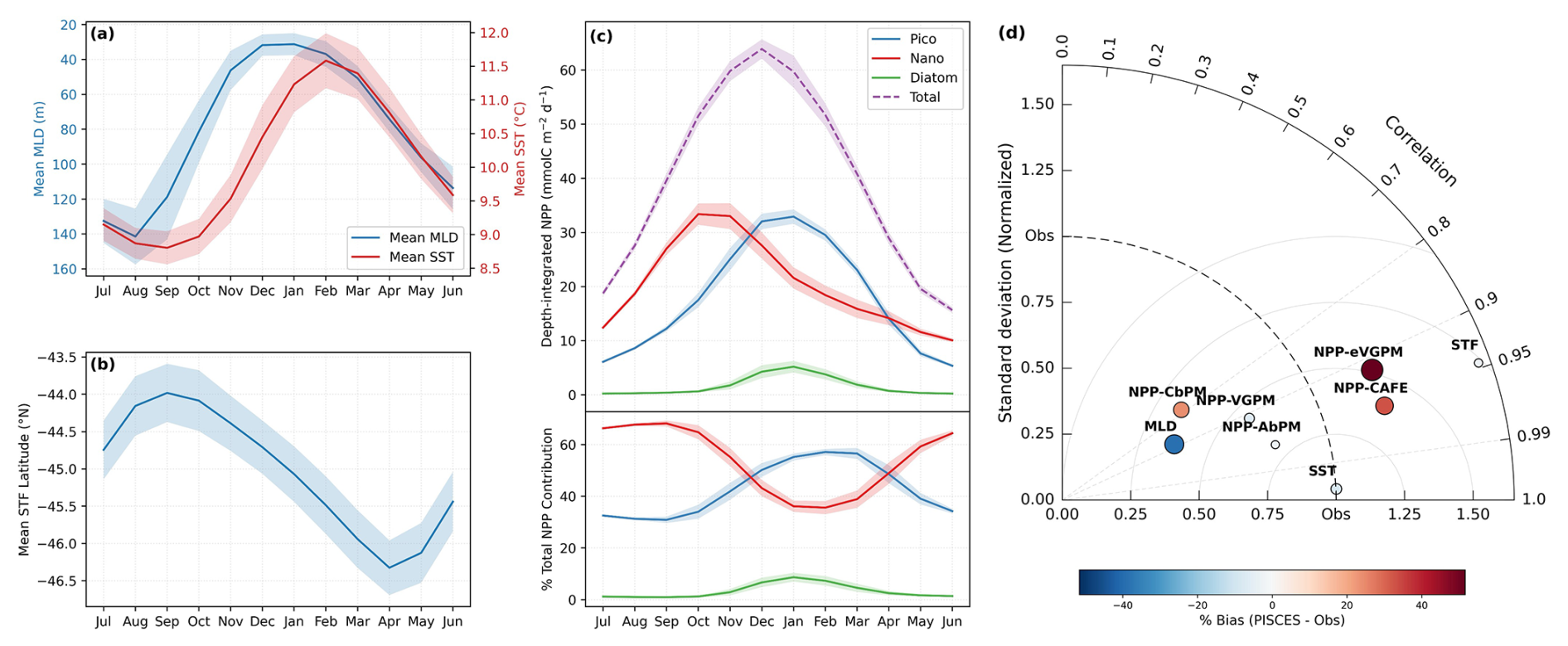
Figure 3 (a) Mean climatological MLD (blue) and SST (red), (b) STF mean latitude in the longitude range 140–150° E extent, and (c) phytoplankton class and total resolved depth-integrated NPP, including percentage contribution of each class to the total NPP inventory, and (d) Taylor diagram summarising climatological differences between NPP, MLD, SST and STF latitude between PISCES-Quota-Fe and observations for the period 1998–2023. Relative bias (%) is given as marker size and colour denoting bias direction.

The relationships between drivers and NPP in PISCES-Quota-Fe (Fig. 4a–d) were generally more consistent with CbPM, CAFE and AbPM remote sensing algorithms than VGPM and eVGPM algorithms (cf. Fig. 2). Of the physical drivers examined in PISCES-Quota-Fe, variability in temperature and STF location did not dominate as drivers of NPP interannual variability (Fig. 4c, d). Climatological ΔSST was consistently negative during high NPP periods but only significant in March when negative ΔSST peaked (Fig. 4c). Cooler temperatures between high and low NPP seasons were observed during summer but were insignificant, except in the surface 75 m in March (Fig. 4e). STF latitude did not vary significantly between high and low NPP periods (Fig. 4d), despite cooler temperatures co-occurring with a northern shift in the STF in spring and late autumn. While this was more consistent with CbPM, CAFE and AbPM NPP algorithms than VGPM/eVGPM (Fig. 4d), variability in simulated NPP is not statistically linked to increases in subtropical water mass presence in this region.

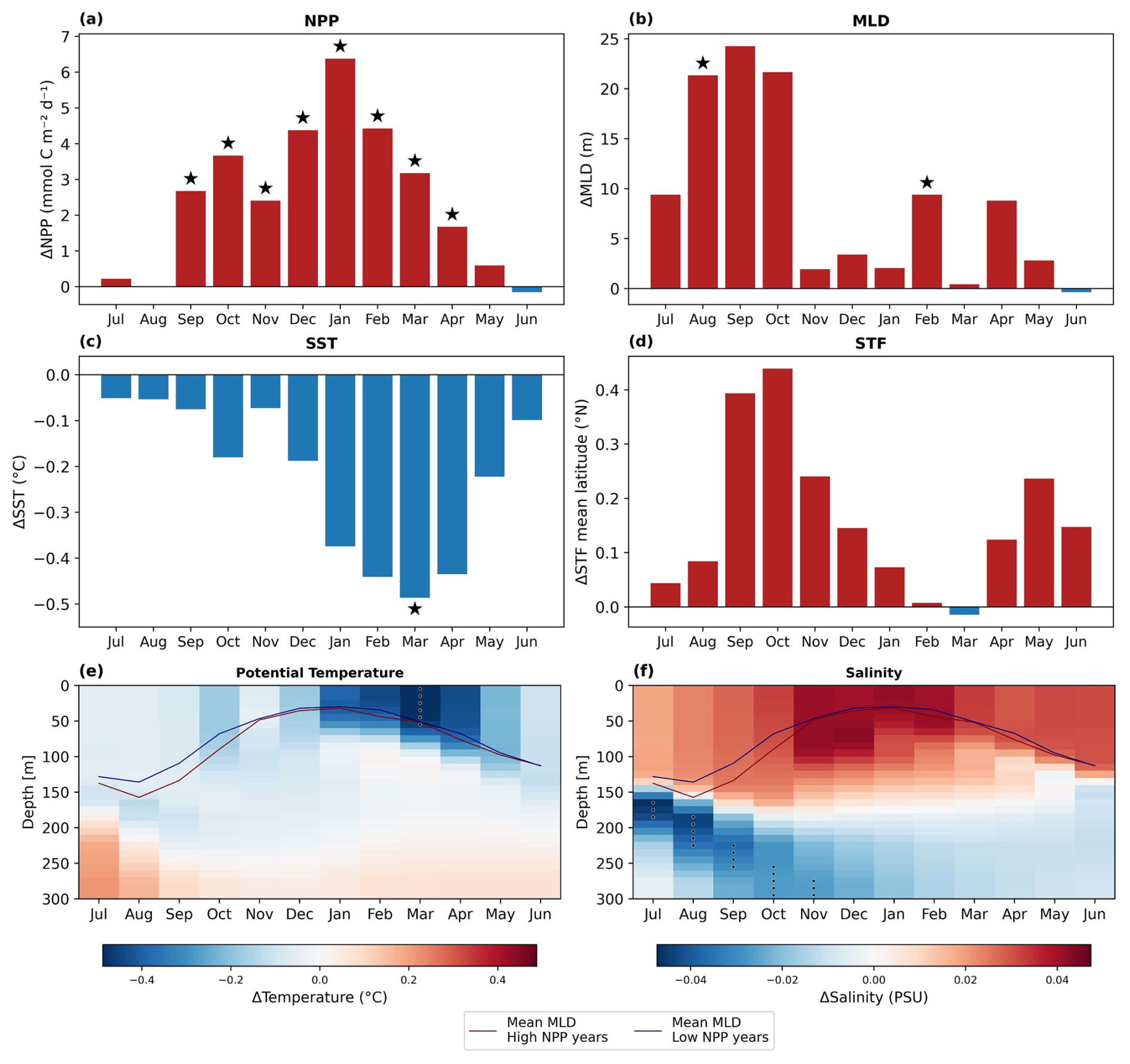
Figure 4 Mean Monthly climatological differences in NPP (a) and simulated physical drivers of ΔMLD (b), ΔSST (c) and ΔSTF mean latitude (d), and depth resolved (interpolated onto a 10 m regular depth grid) Δ potential temperature (e) and Δsalinity (f) between high and low total integrated NPP seasons. Stars and stippling indicate that mean monthly climatological difference in the selected high and low NPP season groups is significant relative to the full time series climatological variability at the p<0.05 level (10 000 iteration random year bootstrapping analysis). Red and blue solid lines denote mean MLDs in respective high and low NPP year groups.

In high NPP years, MLDs were generally deeper in winter through to spring and sporadically in summer and autumn, with significantly positive ΔMLD only in August and February (Fig. 4b). However, ΔMLD was very small from November to January and during March (Fig. 4b), months where positive total ΔNPP was strongest (Fig. 4a). Changes in mixed layer depth during spring may have a lasting memory effect into summer by modifying mixed layer nutrient, light and predator-prey interactions.

Indeed, higher NPP seasons were associated with significant increases in NO₃, Si and DFe mixed layer inventories (Fig. 5a, b, c). The average (biomass-weighted) community composition showed a clear iron limitation signal during the productive season (Fig. A1 in the Appendix), with the exception of picophytoplankton that were generally nitrogen limited (Fig. A2 in the Appendix).

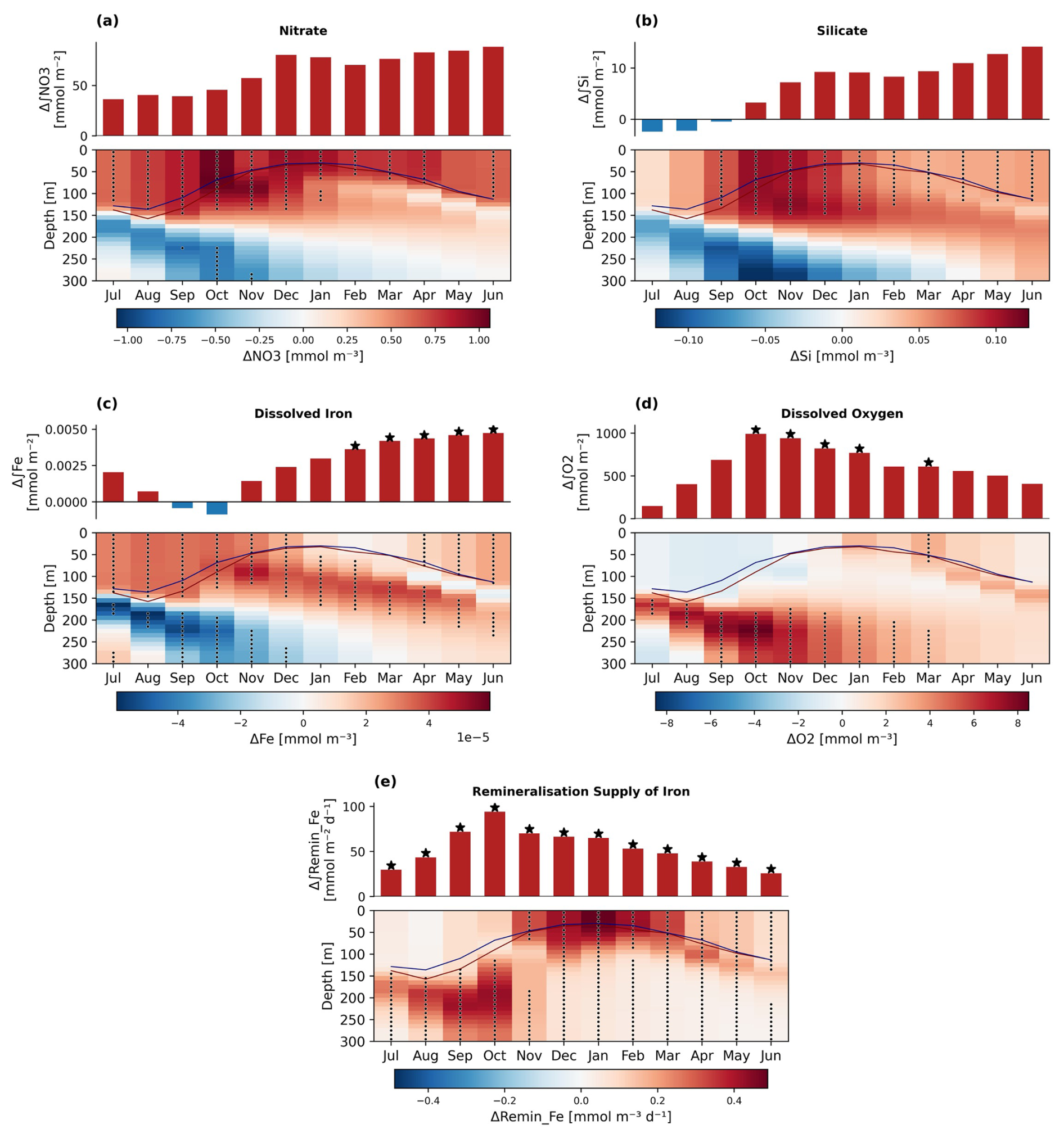
Figure 5 Climatological difference in simulated mean nutrient water column inventories (bar plots) and depth resolved concentration differences interpolated onto a 10 m regular grid (heatmaps) for (a) ΔNO₃, (b) ΔSi, (c) ΔDFe, (d) ΔO₂, and (e) the difference in the rate of remineralised iron supply (ΔRemin_Fe) between high and low NPP seasons. Stars and stippling indicate that mean monthly climatological difference in the selected high and low NPP season groups is significantly outside the full time series climatological variability at the p<0.05 level (10 000 iteration random year bootstrapping analysis). Red and blue solid lines denote mean MLDs in respective high and low NPP year groups.

3.3 Variability in simulated NPP is decoupled from biomass

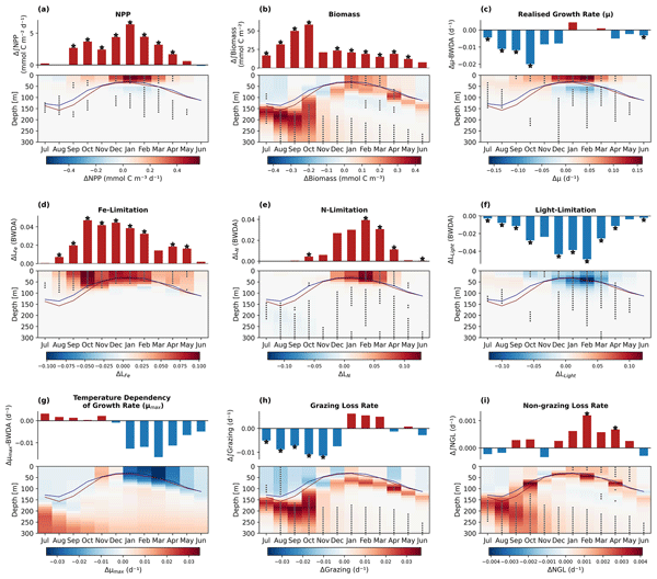
While the largest ΔNPP (Fig. 6a) generally corresponded to positive ΔBiomass, predominantly driven by significantly increased nanophytoplankton ΔNPP (Fig. 6a) and corresponding nanophytoplankton biomass (Fig. 6b), climatological changes in total biomass and NPP were not directly correlated. Total ΔBiomass was largest in spring, while ΔNPP was largest in January. This increase in total spring biomass occurred despite significantly reduced total phytoplankton division rates (µ) from July to October (Fig. 6c). In summer, ΔBiomass was still significantly increased in high NPP years (December to March), indicating sustained elevated biomass contributed to NPP in summer (Fig. 6a, b) while total average growth rates (µ) did not change significantly (Fig. 6c).

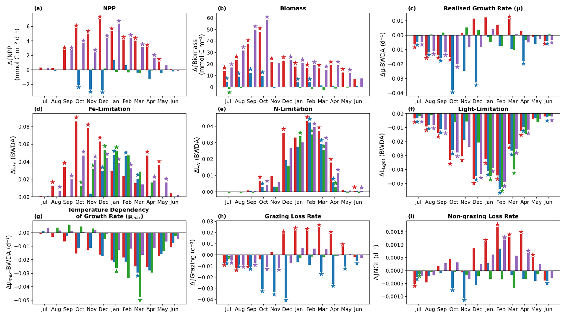
Figure 6 Simulated changes (Δ) in phytoplankton class specific and total mean climatological terms determined from the mean climatological difference between high and low integrated total NPP seasons for: (a) depth integrated ΔNPP, (b) depth integrated ΔBiomass, (c) biomass-weighted depth-averaged growth rate Δµ, (d) biomass-weighted depth-averaged iron limitation, ΔL_Fe, (positive ΔL_Fe indicates reduced iron limitation), (e) biomass-weighted depth-averaged nitrogen limitation ΔL_N (positive ΔL_N indicates reduced nitrate limitation), (f) biomass-weighted depth-averaged light limitation ΔL_light (negative ΔL_Light indicates increased light limitation), (g) biomass-weighted depth-averaged growth rate temperature dependency µ_max, (h) phytoplankton biomass normalized specific grazing loss rate ΔGrazing, and (i) phytoplankton biomass normalized specific non-grazing loss rate ΔNGL. Stars denote that mean monthly climatological difference in the selected high and low NPP season groups is significantly exceeds the full time series climatological variability at the p<0.05 level (10 000 iteration random year group bootstrapping analysis).

In determining why decreases in spring division rates emerge in high NPP periods, we found lower temperatures are unlikely to be the dominant driver of reduced growth rates. Assessment of the growth rate temperature dependency (µ_max) showed that while negative Δµ_max occurred with lower temperatures during high NPP periods (Fig. 4c, e), Δµ_max was not significantly reduced for the total phytoplankton population over the climatology (Fig. 6g). To evaluate why average phytoplankton division rates (µ) decreased in spring despite increased NPP, we investigated the explicit depth resolved limitation terms that drive phytoplankton growth rates and thus biomass evolution and NPP responses.

3.4 Multiple competing mechanisms associated with MLD drive interannual variability in simulated NPP

In higher NPP years, biomass-weighted depth-averaged realised growth rates (Δµ) were significantly reduced from July to October (Fig. 6c). The co-existence of higher NPP despite poorer growth conditions for the average phytoplankton requires the role of either top-down processes affecting biomass loss rates or a physical decoupling between where changes in biomass and growth rates occur in the water column in response to bottom-up processes. Both top-down and bottom-up roles regulated interannual variability in NPP, but their relative influence changed throughout the productivity season.

We found that increased NPP during the spring arose from the unique ways in which bottom-up and top-down processes responded to deeper mixing. Initially, strong bottom-up controls linked to relief of iron limitation appeared to drive increased NPP. Fe limitation was reduced through July–November, with consistently and significantly increased class specific and total phytoplankton community averaged L_Fe terms in high NPP years (Fig. 6d). This effect was confined to depths from the surface to just below the mixed layer (Fig. 7d), following increased mixed layer DFe inventories (Fig. 5c). Increased DFe mixed layer inventories during spring were not from remineralised iron sources (Fig. 5e), suggesting that springtime relief of iron limitation was driven by entrainment. Significantly higher depth resolved Δµ within the mixed layer reflected these better growth conditions for the average phytoplankton (Fig. 7c). This corresponded to increases in surface NPP (Fig. 7a), despite a non-significant increase in surface biomass during the July-November period (Figs. 7b, A3, A4, A5).

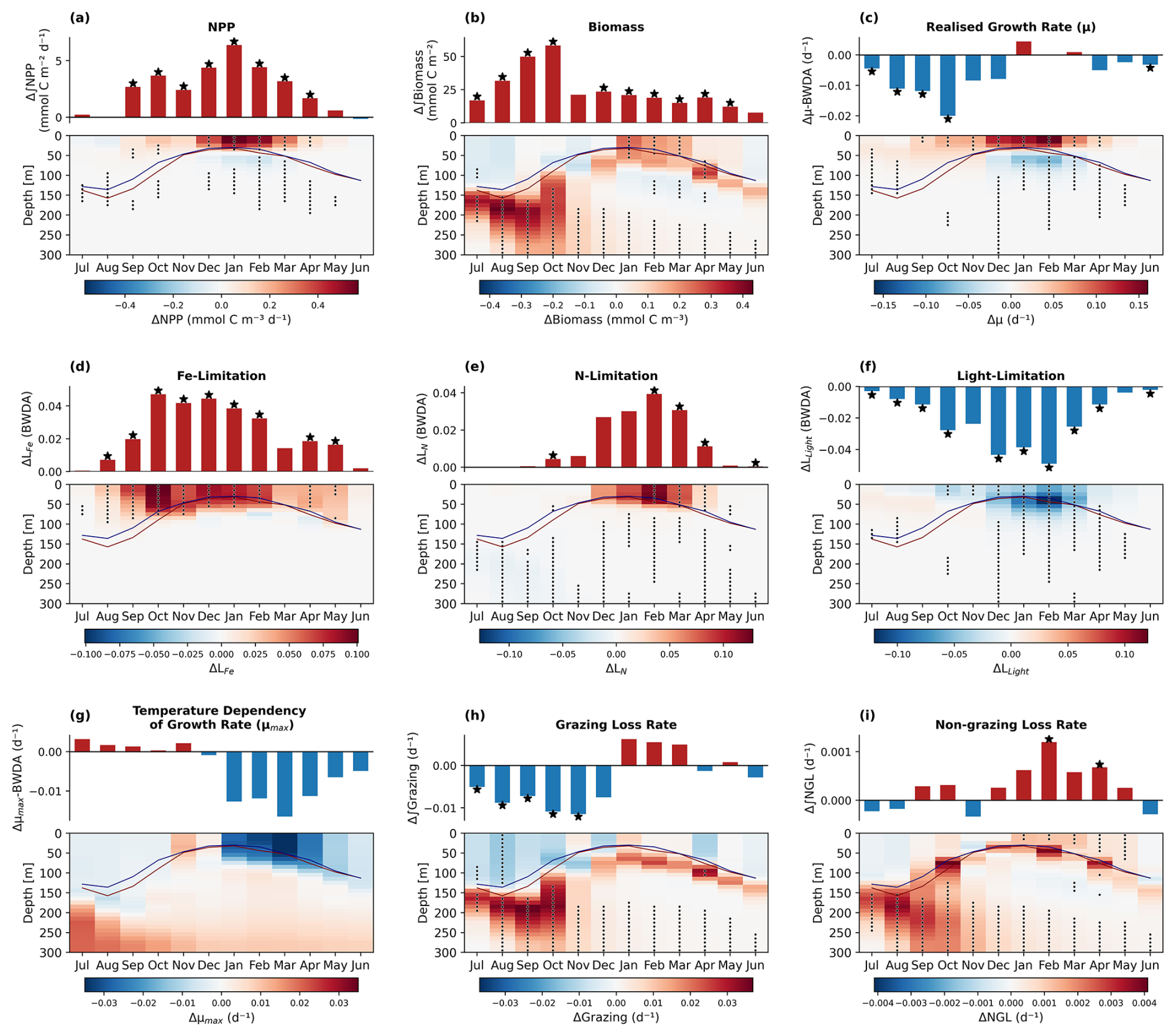
Figure 7 Simulated integrated (bar plots) and depth resolved (interpolated onto a 10 m regular grid) mean climatological (a) ΔNPP, (b) ΔBiomass, (c) biomass-weighted depth-averaged growth rate Δµ , (d) biomass-weighted depth-averaged iron limitation, ΔL_Fe, (e) biomass-weighted depth-averaged nitrogen limitation ΔL_N, (f) biomass-weighted depth-averaged light limitation ΔL_light, (g) Biomass-weighted depth-averaged growth rate temperature dependency µ_max, (h) phytoplankton biomass normalized specific grazing loss rate ΔGrazing, and (i) phytoplankton biomass normalized specific non-grazing loss rate ΔNGL. Δ terms were determined from the mean climatological difference between high and low integrated total NPP seasons. Stars and stippling denote that mean monthly climatological difference in the selected high and low NPP season groups significantly exceeds the full time series climatological variability at the p<0.05 level (10 000 iteration random year bootstrapping analysis). Red and blue solid lines denote mean MLDs in respective high and low NPP year groups.

However, increased phytoplankton division rates within the mixed layer did not translate to increased biomass Fig. 7b, c), because deeper mixing drove biomass below the mean monthly mixed layer. The redistribution of simulated phytoplankton biomass to depth led to additional top-down controls on phytoplankton biomass accumulation into summer, possibly through the destabilizing properties of the prescribed grazing functional response (Gentleman and Neuheimer, 2008; Rohr et al., 2022). Between high and low NPP periods, depth-integrated biomass significantly increased in spring (Fig. 7b), while total grazing loss rates significantly decreased (Figs. 7h, A3, A4, A5) with decreasing zooplankton biomass (Fig. A6). Resolved over depth, the reduction in grazing loss rates was strongest in the mixed layer (Fig. 7h). While grazing rates decreased, total mixed layer phytoplankton biomass remained the same (or significantly decreased in the cases of picophytoplankton and diatoms, Figs. A4, A5), while below the mixed layer, biomass increased (Fig. 7b).

The significant deep biomass anomalies below the mean monthly MLD (Fig. 7b) were likely due to synoptic scale mixing events averaged out in mean monthly MLD. This redistribution of phytoplankton biomass significantly reduced grazing loss rates in the mixed layer (Fig. 7h), alongside reduced micro- and mesozooplankton biomass (Fig. A6e, f). This reduction in top-down loss pressure likely contributed to increased mixed layer NPP by reducing grazing pressure in the mixed layer where growth conditions were enhanced, while also mitigating biomass losses to detrainment. These results highlight that higher spring NPP can occur despite biomass-weighted depth-average decreases in µ (Fig. 6c, 7c) that arise from shifting biomass to greater depth where growth conditions were unfavourable due to insufficient light (Fig. 7f).

Following shoaling of the mixed layer in spring/summer, high NPP years were associated with divergent changes to growth conditions above and below the mixed layer. Higher NPP seasons were consistently linked to surface changes in growth conditions and biomass (Fig. 7). In the mixed layer, growth conditions improved (Fig. 7c), due to relief of iron limitation (Figs. 7d, A2). This occurred despite significantly increased light limitation (Fig. 7f). Cooler temperatures reduced the thermal growth rate dependency but not significantly between high and low NPP seasons (Fig. 7g). Both DFe and NO₃ inventories were significantly higher through summer (Fig. 5), reducing nutrient limitation and driving positive Δµ in the mixed layer (Fig. 7d, e). Importantly, increased supply of remineralised iron was significantly increased in the mixed layer (Fig. 5e), maintaining iron limitation relief following mixed layer shoaling. The improved mixed layer growth conditions led to higher biomass (Fig. 7b) and NPP (Fig. 7a). Notably, summertime biomass-weighted depth averaged Δµ , which was not significantly different between high and low NPP seasons, reflected poorer growth conditions below the mixed layer (Fig. 7a, c, f).

3.5 Environmental drivers of subantarctic NPP in CMIP6 models

In the highest NPP years, increased SSTs and more southern STF position were generally consistent across the whole year for ACCESS-ESM1.5, CanESM5-CanOE, CanESM5-CMOC, CESM2 and CMCC-ESM2 models, suggesting that thermal drivers dominated highest NPP years for this subset of CMIP6 models (Fig. 8c). In PISCES-v2 containing models IPSL-CM6A and CNRM-ESM2-1, SSTs were only significantly warmer from July to October (Fig. 8c), which opposes our findings of cooler SSTs in PISCES-QUOTA-FE assessment (Fig. 4c). Despite generally warmer SSTs, the significant differences between highest and lowest NPP year groups in CMIP6 models were variable, with ΔNPP ranging from 2 to 40 mmol C m² d⁻¹ (Fig. 8a). The largest differences in NPP between highest and lowest NPP year groups were in CESM2 and the smallest differences in ACCESS-ESM1.5, CanESM5-CMOC, GFDL-ESM4 and CMCC-ESM2 models (Fig. 8a).

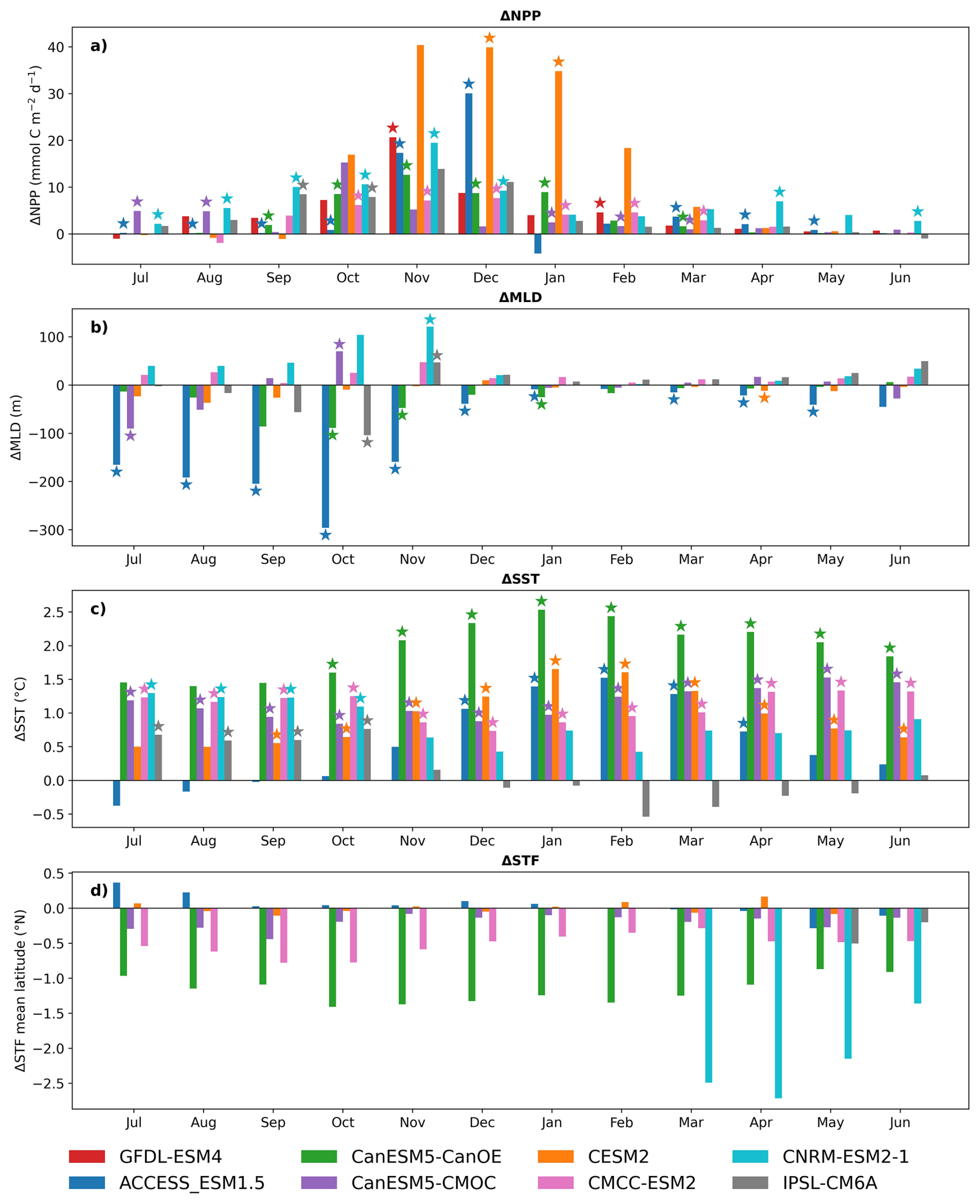
Figure 8 (a) Bootstrap analysis of the change in mean climatological NPP between the 5 highest and 5 lowest seasons of NPP for 8 CMIP6 models listed in Table 2 (note SST and MLD not available for GFDL-EMS4). (b–d) Change in MLD, SST and STF mean latitude correspond to mean climatological changes based on respective model high and low NPP season groups in (a). SST and MLD not available for GFDL-ESM4 output. Stars denote trends significantly different from zero at the p<0.05 confidence level.

Between highest and lowest NPP year groups, ΔMLD was large and varied substantially across models (Fig. 8b). Through winter and spring, ACCESS-ESM1.5 ΔMLD was significantly shallower than any other model, with ΔMLD values ranging from 100 to 300 m shallower. During high NPP years (Fig. 8b), deeper MLDs were significant for only CanESM5-CMOC in October, and IPSL-CM6A and CNRM-ESM2-1 in November (Fig. 8b). IPSL-CM6A and CNRM-ESM2-1 use PISCES-v2 biogeochemical modules, and deeper MLDs in November are consistent with our assessment of PISCES-QUOTA-FE.

4 Discussion

4.1 Does our understanding of simulated drivers of NPP help explain remote-sensing NPP algorithm divergence?

The inconsistent relationship between NPP and environmental drivers seen across VGPM/eVGPM and CbPM/AbPM/CAFE algorithms is also observed in previous Southern Ocean assessments (Pinkerton et al., 2021; Ryan-Keogh et al., 2025b; Tagliabue et al., 2025). This inconsistency between remote sensing NPP algorithms suggests uncertainty around the mechanistic links between drivers and NPP. This uncertainty may arise from potential biases in how NPP is derived from biomass and growth rates, or more complex competing mechanistic relationships than can be parameterised using first-order relationships of surface ocean environmental variables.

The interannual variability in NPP in our biogeochemical model was linked to variability in winter/spring MLD, driving cascading changes to the bottom-up and top-down controls and demonstrating how decoupling between biomass and growth rates (µ) can arise. For remote sensing NPP algorithms, the CAFE and CbPM algorithms both include MLD. The CbPM algorithm also includes nitracline depth to determine nitrate limitation based on the proximity of MLD and nitracline depths (Westberry et al., 2008; Ryan-Keogh et al., 2023a). However, differences in climatological ΔNPP across CAFE and CbPM algorithms are likely driven by differences in how biomass, chlorophyll and absorption spectra are incorporated into respective algorithms (Fig. 2).

Our investigation of remote sensing algorithms did not find consistent and significant links between deeper MLDs in spring and increased NPP. Rather, the only significant relationship identified was in the CbPM algorithm, where shallower MLD was correlated with increased NPP in October and November (Fig. 2). While this relationship was also indicated in the VGPM, eVGPM and CAFE algorithms, it was not significant (Fig. 2). This does provide some indication that earlier shoaling of the MLD enhanced light availability for mixed layer productivity, consistent with observations of light as a seasonal productivity driver in this region (Trull et al., 2019). This effect in the CbPM algorithm was not sustained through to summer however, indicative that algorithm sensitivity to light attenuation forms only part of mechanistic NPP variability and was confined to spring.

The absence of stronger or more widespread relationships in remote sensing products may arise from several factors. First and most importantly, the complexity of mechanisms driving interannual NPP variability captured in the coupled physical–biogeochemical model likely reflects realistic, nonlinear interactions among physical processes, light, nutrients, and grazing. These processes often counteract one another, resulting in weak net effects that are difficult to detect in surface-constrained observations. Secondly, remote sensing algorithms rely on simplified parameterisations that may exclude subsurface processes critical to NPP variability, or biases in input variables (Saba et al., 2011). Third, the averaged MLD product may not accurately resolve sub-seasonal variability in MLD which is an important driver of SAZ primary production (Swart et al., 2015, 2023). The last possibility is that the mechanisms generated in the model are poorly representative of the in-situ system. As such, the lack of consistent relationships does not imply an absence of physical–biological coupling but rather highlights the limitations of simplified remotely-sensed algorithms in resolving emergent and interacting drivers of phytoplankton biomass and growth rates.

4.2 Bottom-up and top-down drivers of NPP are linked by ecosystem functional responses

The uncertainty in environmental drivers of observed NPP likely occurs due to the many competing controls on biogeochemistry. Changes to the MLD in the Southern Ocean affects NPP by altering both nutrient and light availability in generally opposing directions. Deeper mixed layers entrain nutrients from below but also reduce light availability to phytoplankton that are mixed deeper in the water column (Tagliabue et al., 2014; Deppeler and Davidson, 2017; Llort et al., 2019). The timing of MLD shoaling, relative to seasonal changes in incoming radiation and SST also determines the response of the phytoplankton community (Deppeler and Davidson, 2017), as observed here in PISCES-Quota-Fe.

In PISCES-Quota-Fe, the climatological average productivity response to changes in MLD was complicated through competing changes in ecosystem structure and top-down controls. Firstly, the responses of phytoplankton to bottom-up controls (class specific nutrient limitation) varied between groups, where reduced iron limitation in high NPP seasons allowed the strongest NPP contribution from nanophytoplankton as the dominant phytoplankton group over picophytoplankton and diatoms (cf. Figs. A3, A4, A5). And second, the decoupling between changes in the MLD and NPP over the climatological cycle was exacerbated by the response of grazers to changes in the prey field as dictated by their prescribed functional response curves.

In our results, during spring the dilution of biomass over greater depth and the lack of increased biomass in the mixed layer corresponded to reduced grazing (Fig. 7h), preconditioning the mixed layer to this destabilising predator-prey dynamic (Evans and Parslow, 1985; Behrenfeld, 2010). This was likely driven by the rate at which clearance rate, the volumetric rate at which phytoplankton are grazed per unit zooplankton, changes with phytoplankton concentrations (i.e. the speed at which clearance rate changes with respect to changing phytoplankton concentrations). In type II (and circumstantially type III) prescribed functional responses (Gentleman et al., 2003; Gentleman and Neuheimer, 2008), clearance rates decrease with biomass accumulation during seasonal bloom formation as grazing becomes less efficient per unit zooplankton (Gentleman and Neuheimer, 2008; Rohr et al., 2022). This reduced grazing efficiency allows more rapid phytoplankton biomass accumulation, destabilizing grazing as a top-down control in the predator-prey dynamic (Gentleman and Neuheimer, 2008; Rohr et al., 2022).

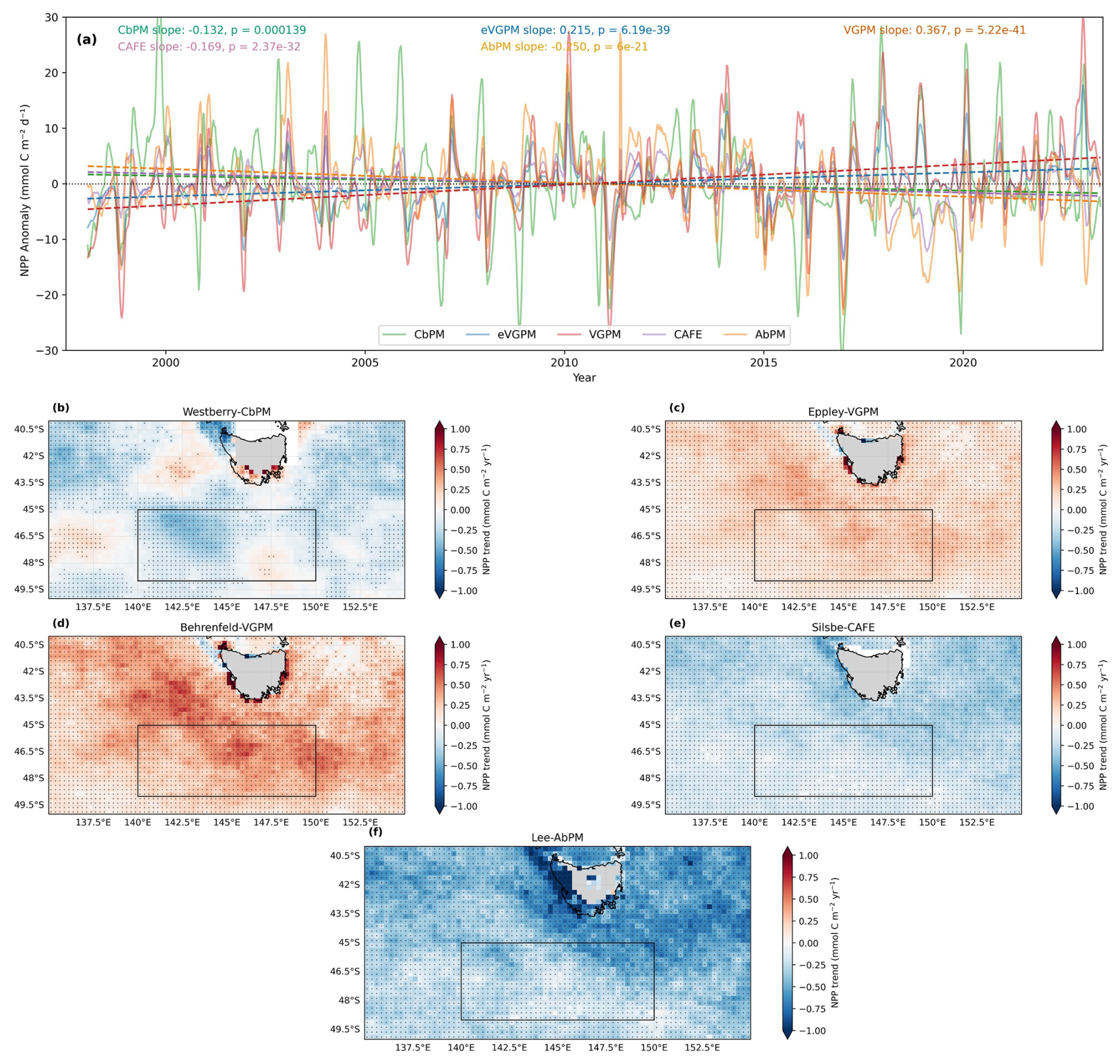
Figure 9 (a) Timeseries (1998–2022) of monthly NPP anomalies from the five remote sensing NPP algorithms, spatially averaged over the SOTS region (45–49° S, 140–150° E). Trends were determined from ordinary least squares regression of the monthly anomalies, with trend slope and p-values for significance given. (b–e) Spatial trends computed from ordinary least squares regressions on monthly single pixel NPP anomalies for each remote sensing NPP algorithm in (a). Stippling in pixels indicates significant rends at the p<0.05 level. The black box denotes study region used for averaging in (a).

The impact of a more destabilising functional response amplifies changes in phytoplankton growth, which under reduced grazing loss rates, primes the growing population to greater potential growth ahead of increasing zooplankton population (Rohr et al., 2022). These properties likely contributed to significantly increased mixed layer biomass accumulation from January to March, when peak ΔNPP occurs, despite the same or lower biomass in the spring during initiation (Fig. 6b, 7b), and a lack of significant changes to summer grazing loss rates (Fig. 7h). Indeed, clearance rates for the average phytoplankton in the mixed layer significantly decreased in summer (Fig. A6) despite significantly increased summer mixed layer biomass (Fig. 7b).

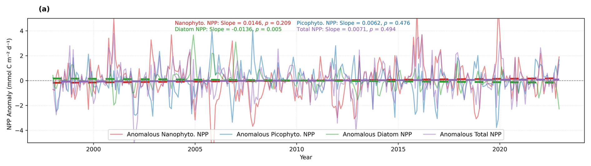
Figure 10 (a) PISCES-Quota-Fe simulated class specific NPP monthly anomalies (thin lines), fitted with ordinary least squares trend regressions for the period 1998–2022 corresponding to the remote sensing record. (b) Extended NPP trend analysis over the full study simulation time series 1975–2022.

To assess the intrinsic stability of the predator-prey functional response in PISCES-Quota-Fe, determination of the first order stability of the functional response, calculated from the rate of change in clearance rate as prey density increases, is required to assess the nonlinear way in which clearance rate changes with mixed layer reduced biomass (Gentleman and Neuheimer, 2008; Rohr et al., 2022). Unfortunately, the multispecies predator-prey system of PISCES-Quota-Fe challenges post-hoc quantification of inherent changes in stability from the rate of clearance rate changes with respect to phytoplankton concentration. This is due to multiple grazing rates across multiple phytoplankton groups and concentrations, driving differential phytoplankton loss rates that are lost across monthly and group averages. Nevertheless, we can be confident that the changes in grazing loss rates follow patterns in prey biomass distributions, instigated by deepening of the mixed layer, and favouring biomass accumulation and increased NPP in the surface moving into summer.

4.3 Implications for NPP trends in historical observation and model projections

When we examined trends in the remotely-sensed NPP record (monthly anomalies 1998–2022), the divergence between significantly positive trends in VGPM/eVGPM algorithms and negative trends in CbPM, AbPM and CAFE algorithms was clear (Fig. 9a), reflecting the disparity in their parametric derivation. This is supported by previous work investigating the emergence of broader Southern Ocean trends based on remote sensing NPP algorithms, with similarly divergent NPP trends between VGPM and CbPM algorithms (Pinkerton et al., 2021; Ryan-Keogh et al., 2023b, 2025a). Trends in VGPM and eVGPM algorithms (Fig. 9c, d) are particularly sensitive to start and end dates owing to climate modes, more so because they are driven by trends in surface chlorophyll and SST associated with Southern Ocean warming (Henley et al., 2020; Ryan-Keogh et al., 2023b). Trends in CbPM NPP were spatially heterogenous (Fig. 9b), reducing confidence in the overall negative trend (Fig. 9a).

In their comparison of OC-CCI based NPP algorithms, Ryan-Keogh et al. (2025b) suggested that more robust assessment of NPP drivers can be achieved with CAFE and AbPM algorithms, as these models have better agreement with field observations (Lee et al., 2011; Saba et al., 2011; Wu et al., 2024; Ryan-Keogh et al., 2025b). Additionally, the light absorption efficiency parametrisation in AbPM and CAFE algorithms better reflects NPP responses to environmental conditions compared to the strong influence of temperature on metabolic rates in eVGPM and VGPM algorithms (Ryan-Keogh et al., 2025b). The validation of the best NPP algorithm in this region is beyond the scope of this study, but based on previous algorithm intercomparison, in-situ trends in this part of the SAZ region are very likely to reflect decreasing NPP as in AbPM, CAFE, CbPM algorithms (Fig. 9).

For the same period as the remote sensing record (1998–2022), in the PISCES-Quota-Fe hindcast simulation, no significant trends in total monthly NPP anomalies were identified (Fig. 10a), with the exception of a significant trend in decreasing diatom NPP. However, extension of the trend analysis to the full time series used to assess mechanistic drivers of NPP (1975–2022) indicated significantly positive trends in total NPP, driven by increasing nanophytoplankton NPP (Fig. 10b). A concomitant reduction in iron limitation was confirmed as a significant trend (Fig. A7). This sensitivity of trend analysis to time series length, start and end dates may limit our ability to confidently identify NPP trends and mechanisms driving interannual variability in both observational and simulated time series (Elsworth et al., 2020; Kwiatkowski et al., 2020).

However, the convergence of increasing trends in simulated NPP in this study region in both PISCES-Quota-Fe and historical CMIP6 models, with the exception of ACCESS-ESM1.5 (Fig. A8), and similarly reported Southern Ocean NPP projected increases elsewhere (Fisher et al., 2025; Ryan-Keogh et al., 2025b), suggests that biogeochemical models are reasonably consistent in the direction of future NPP projections despite significant uncertainty in the magnitude. Our mechanistic understanding of PISCES-Quota-Fe links increasing NPP with a reduction in iron limitation and destabilising predator-prey dynamics. CMIP6 NPP increases are generally associated with a trend in reduced iron limitation (Tagliabue et al., 2021) but is complicated by indirect diagnosis of iron limitation term impacts on phytoplankton growth rates and NPP (Tagliabue et al., 2025). Without explicit growth limitation terms from biogeochemical module componentry saved for historical CMIP6 models, there remains large uncertainty surrounding the full suite of environmental drivers. This is particularly the case with variability between models in the direction of ΔMLD during high NPP years (Fig. 8b) yet consistently increased ΔSSTs suggesting thermally driven NPP trends (Fig. 8c). Moreover, broad variability in the difference between highest and lowest NPP years in CMIP6 models (Fig. 8a) highlights that NPP response mechanism to warmer temperatures vary broadly.

The convergence of model predictions indicating increasing NPP and decreasing iron limitation reported here and across the literature has important implications for addressing trend interpretations and observationally constrained model development. The findings of models is at odds with prior observations indicate decreasing NPP trends and increasing iron stress over the remote sensing record (Ryan-Keogh et al., 2023b). The uncertainty in mechanistic relationships between remote sensing algorithms, PISCES-Quota-Fe and CMIP6 simulations urges a cautionary interpretation of trends emerging in both observationally and simulated methods.

As such, further improvement to our understanding of mechanistic processes is required to constrain modelled biogeochemical and ecological systems relative to observed trends. With regards to addressing mechanistic knowledge gaps in NPP drivers, the processes of resource limitation, zooplankton dynamics and phytoplankton loss are identified as key priority areas for improving biogeochemical predictive capability (Rohr et al., 2023; Henson et al., 2024; Fisher et al., 2025). Our findings are directly applicable to these areas, giving critical insight into the specific processes that need, and can, be addressed with observational approaches (Tagliabue et al., 2021; Hutchins and Tagliabue, 2024; Fisher et al., 2025).

5 Conclusions

Our analysis identified that in the SAZ south of Australia, remote sensing NPP algorithms showed inconsistent relationships between environmental drivers and interannual NPP variability. Moreover, divergence in both the indicative drivers and NPP trends showed that mechanistic relationships are not consistently represented between algorithms. While this is in part due to the exclusion of biogeochemical and ecological mechanisms in remote sensing algorithms, these estimates are still essential tools in assessing the impact of climate change on productivity systems. In this regard, our analysis supports greater confidence in CbPM, AbPM and CAFE NPP algorithms that integrate physical and optical parameters for estimating of large-scale Southern Ocean productivity change. Future observational efforts should focus on constraining the distinct bio-optical properties (e.g. Fig. 2 legend) in the Southern Ocean towards developing consistent remote sensing NPP algorithms.

To address why decoupling of environmental variables and NPP occur, we used a complex multi-species biogeochemical model to probe the mechanisms that decouple physical environmental drivers as direct controls of NPP variability. These simulations showed that periods of deeper spring mixed layer depth initiates both bottom-up and top-down responses: specifically increasing iron availability by physical and remineralisation supply of Fe, and redistributing/diluting phytoplankton biomass to alter grazing. Together these mechanisms, originate in increased MLD in winter/spring, and sustain nutrient supply into summer to perpetuate increased NPP throughout the season.

Our focus on mechanisms underscores the importance for assessing remotely-sensed derived NPP trends with a degree of caution. The identification of biomass and growth decoupling as a result of altered mixing serves to explain how divergent trends patterns can emerge in NPP algorithm trends due to differences in biomass and growth rates dependencies. Therefore, the assumption of generalised responses of a phytoplankton community to environmental changes may not represent multiple competing community responses that are more sensitive to changes in nutrients, light or grazing, rather than environmental drivers such as temperature and mixing. While incorporating improved productivity system mechanisms into models is needed, concurrent improvement of our understanding of changes in seasonal grazing pressures and multi-resource limitation in the Southern Ocean are both critical components in ground truthing our mechanistic understanding.

When contextualised to historical NPP trends, our understanding of PISCES-Quota-Fe suggests that it and other CMIP6 models generate convergent trends in increasing Southern Ocean NPP that vary in magnitude. The strong bias towards SST trends in several CMIP6 to models is likely due to poorly constrained productivity stabilising mechanisms in models (multi-resource limitation, zooplankton grazing and phytoplankton loss). This understanding is critical since the improvement of biogeochemical models needs to be informed by relevant observational targets that help to constrain biogeochemical feedback processes that account for nutrient, ecological and thermal drivers (Hutchins and Tagliabue, 2024). Moreover the explicit mechanisms identified here are contributing to our understanding of earth system model NPP drivers, and are directly linked to the most important mechanisms that require attention across model intercomparisons (Henson et al., 2024), which can be used to inform future biogeochemical model development. Notwithstanding the need for target mechanistic development in biogeochemical models, observational efforts form a critical part in ground-truthing mechanism concepts. Future observational studies that better constrain changes in seasonal grazing pressures and multi-resource limitation in the Southern Ocean are a critical component towards reciprocal observation-model improvements.

Appendix A

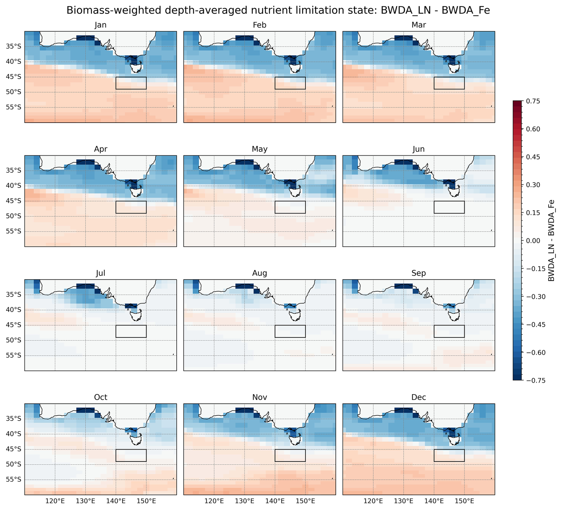
Figure A1 Simulated PISCES-Quota-Fe climatological biomass-weighted depth-averaged difference between L_N and L_Fe limitation terms for the period 1975-2022. Red shading denotes L_Fe dominance (L_Fe<L_N), and blue shading denotes L_N dominance (L_Fe>L_N), defining the nutrient limitation state of phytoplankton classes. Black box denotes study region used to calculate spatial means.

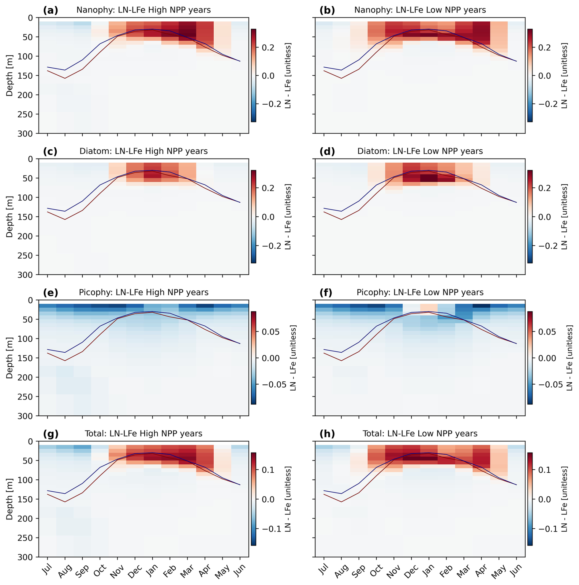
Figure A2 Simulated PISCES-Quota-Fe class specific (nanophytoplankton, diatom, picophytoplankton and community average) depth-resolved biomass-weighted differences between L_N and L_Fe limitation terms averaged for the 5 highest seasonally integrated NPP years (a, c, e, g) and 5 lowest seasonally integrated NPP years from the 1975–2022 time series. Red shading denotes L_Fe dominance (L_Fe<L_N), and blue shading denotes L_N dominance (L_Fe>L_N), defining the nutrient limitation state of phytoplankton classes.

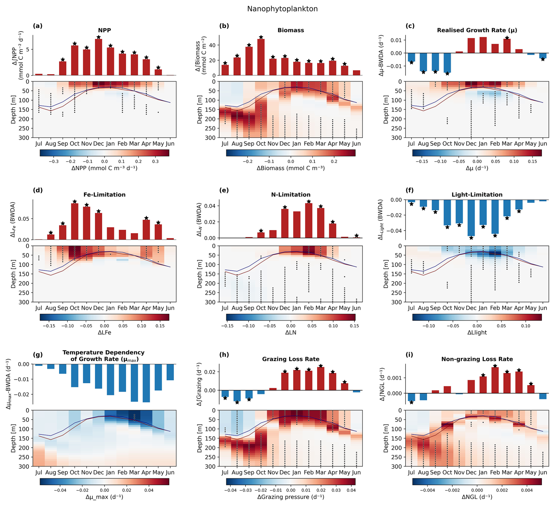
Figure A3 Simulated nanophytoplankton class specific integrated (bar plots) and depth resolved (interpolated onto a 10 m regular grid) mean climatological (a) ΔNPP (b) ΔBiomass, (c) biomass-weighted depth-averaged growth rate Δµ, (d) biomass-weighted depth-averaged iron limitation, ΔL_Fe, (e) biomass-weighted depth-averaged nitrogen limitation ΔL_N, (f) biomass-weighted depth-averaged light limitation ΔL_light, (g) Biomass-weighted depth-averaged growth rate temperature dependency µ _max, (h) phytoplankton biomass normalized specific grazing loss rate, ΔGrazing, (i) phytoplankton biomass normalized specific non-grazing loss rate, ΔNGL. Δ terms were determined from the mean climatological difference between high and low integrated total NPP seasons. Stars denote that mean monthly climatological difference in the selected high and low NPP season groups significantly exceeds the full time series climatological variability at the p<0.05 level (10 000 iteration random year bootstrapping analysis).

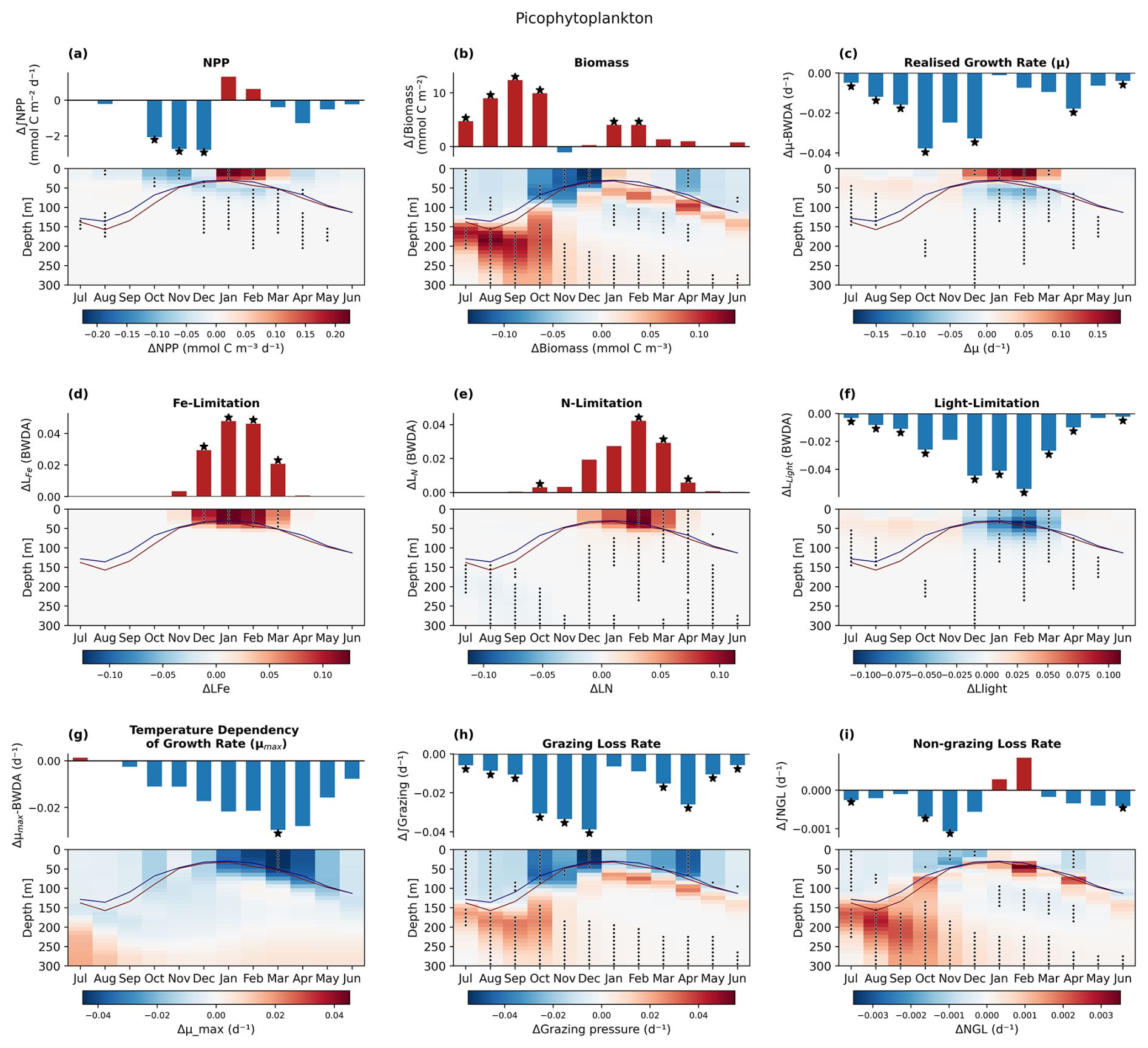
Figure A4 Simulated picophytoplankton class specific integrated (bar plots) and depth resolved (interpolated onto a 10 m regular grid) mean climatological (a) ΔNPP (b) ΔBiomass, (c) biomass-weighted depth-averaged growth rate Δµ, (d) biomass-weighted depth-averaged iron limitation, ΔL_Fe, (e) biomass-weighted depth-averaged nitrogen limitation ΔL_N, (f) biomass-weighted depth-averaged light limitation ΔL_light, (g) Biomass-weighted depth-averaged growth rate temperature dependency µ_max, (h) phytoplankton biomass normalized specific grazing loss rate, ΔGrazing, (i) phytoplankton biomass normalized specific non-grazing loss rate, ΔNGL. Δ terms were determined from the mean climatological difference between high and low integrated total NPP seasons. Stars denote that mean monthly climatological difference in the selected high and low picophytoplankton NPP season groups significantly exceeds the full time series climatological variability at the p<0.05 level (10 000 iteration random year bootstrapping analysis).

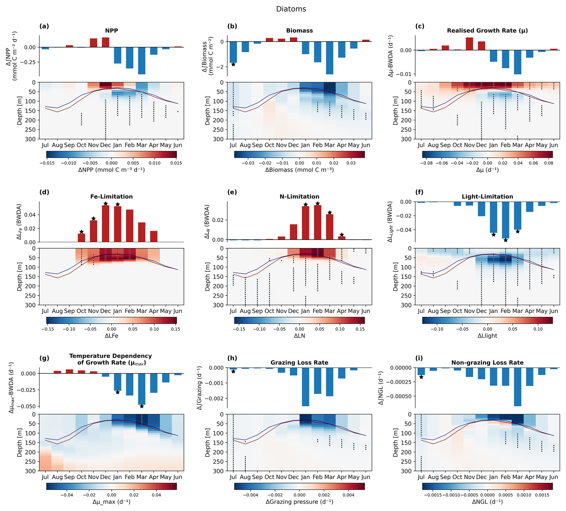
Figure A5 Simulated diatom class specific integrated (bar plots) and depth resolved (interpolated onto a 10 m regular grid) mean climatological (a) ΔNPP (b) ΔBiomass, (c) biomass-weighted depth-averaged growth rate Δµ, (d) biomass-weighted depth-averaged iron limitation, ΔL_Fe, (e) biomass-weighted depth-averaged nitrogen limitation ΔL_N, (f) biomass-weighted depth-averaged light limitation ΔL_light, (g) Biomass-weighted depth-averaged growth rate temperature dependency µ_max, (h) phytoplankton biomass normalized specific grazing loss rate, ΔGrazing, (i) phytoplankton biomass normalized specific non-grazing loss rate, ΔNGL. Δ terms were determined from the mean climatological difference between high and low integrated total NPP seasons. Stars denote that mean monthly climatological difference in the selected high and low diatom NPP season groups significantly exceeds the full time series climatological variability at the p<0.05 level (10 000 iteration random year bootstrapping analysis).

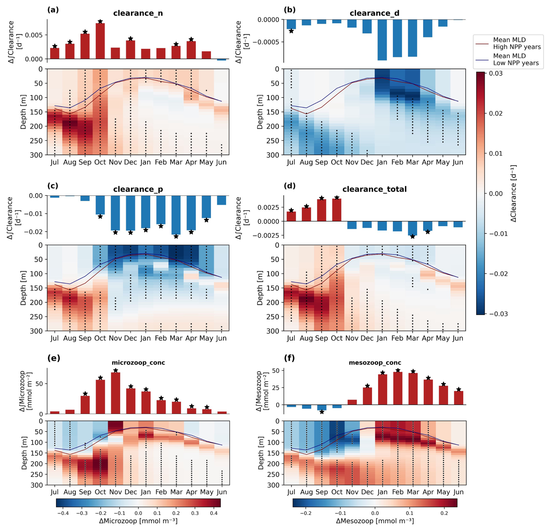
Figure A6 Simulated integrated (bar plots) and depth resolved (interpolated onto a 10 m regular grid) mean climatological clearance rates for specific and total phytoplankton groups. (a) ΔClearance rate for nanophytoplankton, (b) ΔClearance rate for picophytoplankton, (c) ΔClearance rate for diatoms and (d) ΔClearance total phytoplankton (class weighted), and zooplankton biomass (e) ΔMicrozooplankton Biomass, and (f) ΔMesozooplankon Biomass. ΔClearance and ΔZooplankton biomass were determined from the mean climatological difference between high and low integrated total NPP seasons. Stars denote that mean monthly climatological difference in the selected high and low NPP season groups significantly exceeds the full time series climatological variability at the p<0.05 level (10 000 iteration random year bootstrapping analysis).

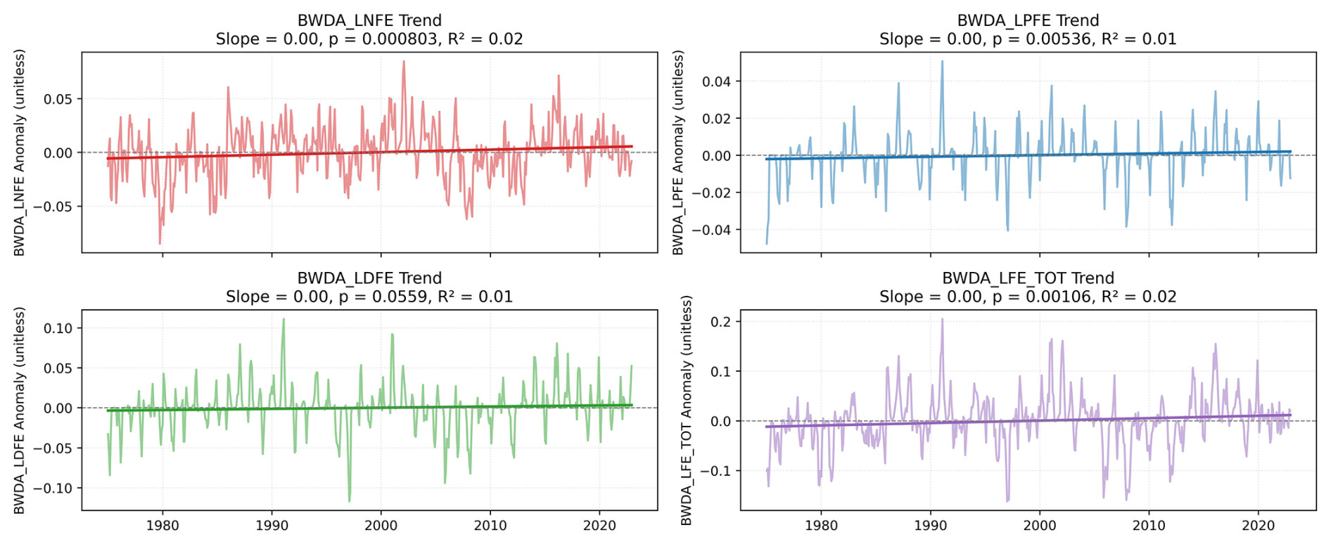
Figure A7 Trends in PISCES-Quota-Fe phytoplankton class specific biomass-weighted, depth-averaged (BWDA) iron limitation terms (positive values indicate decreasing iron limitation).

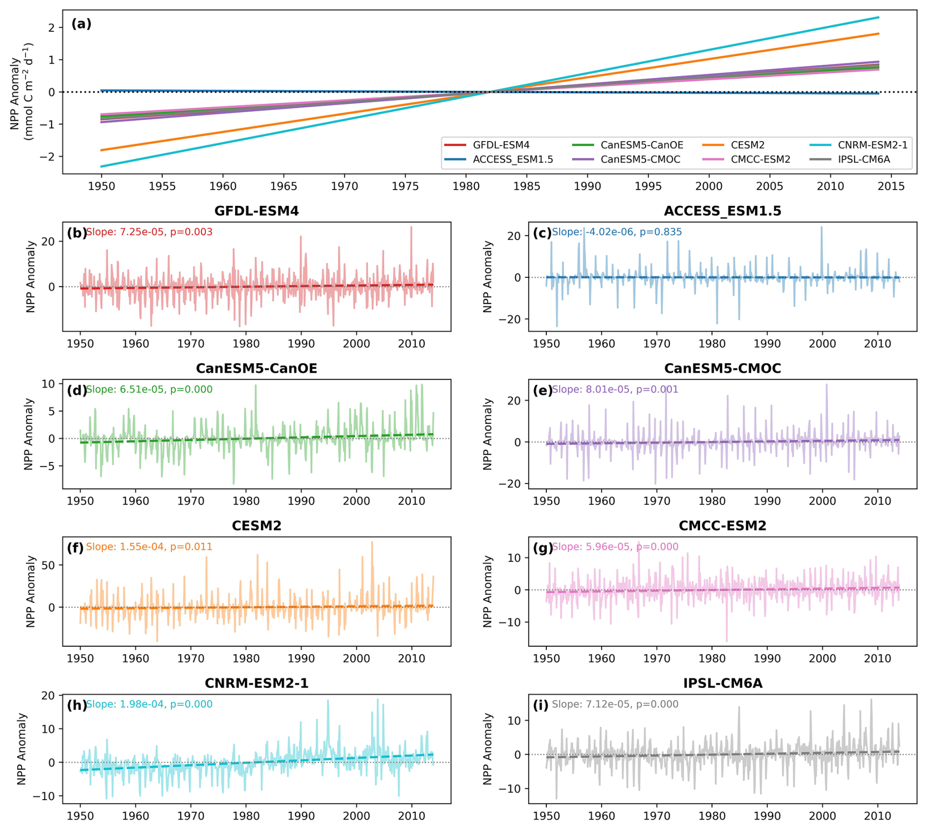
Figure A8 (a) Trends in monthly anomalous NPP time series from the 8 CMIP6 historical models listed in Table 2. (b–i) Individual CMIP6 model time series of spatial mean monthly NPP anomalies. Linear trends were calculated using ordinary least squares regression, with slope and p-values given for trends significantly different from zero (climate modes were not subtracted).