Phenology and surface energy balance changes across northern lands

Plant phenological shifts – notably earlier start (SOS) and later end (EOS) of the growing season – affect surface albedo, latent and sensible heat fluxes, and ultimately the surface temperature. The magnitude and spatial variability of these effects remain uncertain. Using Earth observation and reanalysis data (2001–2021), we quantify the sensitivity of surface energy fluxes to SOS and EOS changes across northern lands (> 30° N), and we report uncertainties and convergence across multiple independent datasets. Spatially-aggregated results show that an earlier SOS is generally associated with decreased albedo by up to 0.003 d⁻¹ (needleleaf forests and tundra), and increased latent heat fluxes by 0.47 $\mathrm{W}{\mathrm{m}}^{-\mathrm{2}}{\mathrm{d}}^{-\mathrm{1}}$ (spatial median), ranging from 0.15 $\mathrm{W}{\mathrm{m}}^{-\mathrm{2}}{\mathrm{d}}^{-\mathrm{1}}$ (croplands) to 0.68 $\mathrm{W}{\mathrm{m}}^{-\mathrm{2}}{\mathrm{d}}^{-\mathrm{1}}$ (mixed forests). Delays in EOS are also associated with decreases in albedo, though much smaller in magnitude, and with increases in latent heat flux – up to ∼0.14 $\mathrm{W}{\mathrm{m}}^{-\mathrm{2}}{\mathrm{d}}^{-\mathrm{1}}$ in mixed forests – with weaker and more variable responses across other land-cover types. Datasets reveal large spatial variability and discrepancies in the responses of the sensible heat fluxes and thus evaporative fraction. Across datasets, earlier SOS is consistently associated with increased latent heat flux, and the concurrent evidence from evaporative fraction suggests a shift towards enhanced latent cooling. These findings are consistent with a phenology-driven negative feedback on surface warming through enhanced evaporative cooling, although causal attribution from observational analyses alone is not possible.

1 Introduction

Across northern vegetated lands, significant shifts in the start date of the growing season (SOS) and end date of the growing season (EOS) have been observed during the last several decades (Piao et al., 2019). The overall more robust plant phenological trends towards earlier SOS have been linked to warming, although there is evidence that the temperature sensitivity of SOS has been declining more recently (Fu et al., 2015). The attribution of the overall weaker trends towards delayed EOS is less clear, and in addition to temperature other factors such as effects from photoperiod, nutrient and water availability also play an important role (Piao et al., 2019).

It is well established that plant phenology exerts a first-order control on water and energy exchanges between the land and atmosphere (Richardson et al., 2013). This is exemplified through in-situ studies documenting that in temperate deciduous forests the seasonal patterns of sensible and latent heat fluxes are largely driven by changes in leaf area index (Moore et al., 1996; Hogg et al., 2000). It is therefore conceivable that shifts in plant phenology have significant impacts on biophysical properties and the surface energy balance during the growing season. For example, through an earlier SOS the foliage cover in springtime is increased, which leads conceivably to a simultaneously enhanced canopy conductance and latent heat fluxes due to increased transpiration of plants (at the cost of sensible heat) as well as altered albedo (Richardson et al., 2013). Further, the increased leaf area also causes an increase in surface aerodynamic roughness, that (through generating more mechanical turbulence) can enhance both sensible and latent heat fluxes (Richardson et al., 2013). Together, these responses can exert large impacts on the springtime near-surface climate (Schwartz and Karl, 1990; Hogg et al., 2000). Additional effects associated with an earlier SOS are decreases in snow cover, soil moisture and surface runoff and potential increases in cloudiness and precipitation as more moisture is expected to be transferred from the land to the atmosphere (Kim et al., 2018; Piao et al., 2019; Mekonnen et al., 2025). A delayed EOS and associated increase in leaf area during autumn may cause similar changes in biophysical properties and imprints in water and energy fluxes, but the overall responses may be more complex because of the influence of changes in energy and water fluxes in the earlier portions of the growing season through lagged effects (Richardson et al., 2010; Liu et al., 2016). Winkler et al. (2026) provide a detailed assessment of how phenological shifts potentially affect the processes controlling land–atmosphere interactions and associated climate feedbacks, given current understanding.

Research on how phenological shifts influence land–atmosphere interactions and near-surface climate has so far primarily focused on land surface temperature responses. In this context, a more recent modeling study by Lian et al. (2022) found that across northern vegetated regions earlier SOS and delayed EOS exert only a relatively modest influence on spring and autumn temperatures, respectively. Their finding suggest that the enhanced evaporative cooling (associated with increased LAI) is largely offset by increased radiative warming associated with albedo changes and water vapor feedbacks.

Shifting the focus to surface energy fluxes, Forzieri et al. (2020) provided the first large-scale observational evidence for a substantial influence of recent leaf area index (LAI) changes on the partitioning of latent and sensible heat fluxes. The study further demonstrated that the ongoing global greening trend – expressed as an increase in annual mean LAI (Winkler et al., 2021) – has led to a decline in the Bowen ratio. This decline was mainly attributed to enhanced evaporative efficiency, particularly in water-limited regions. Prior modeling studies had already reported comparable patterns (Lawrence and Slingo, 2004; Migliavacca et al., 2012), lending additional support to these observational findings.

Analogous to greening effects on the surface energy balance, the overall aim of this study is to quantify the impact of phenological changes in controlling processes. Specifically, the objective is to quantify the direct sensitivities of biophysical properties of the land surface and energy fluxes during the spring and autumn seasons to changes in SOS and EOS for the period 2001–2021 across northern lands. This is an important step towards a better understanding of how phenological shifts in response to climate warming feed back to the climate system (Peñuelas et al., 2009; Miralles et al., 2025b). We make use of an array of newly available datasets of surface energy fluxes and albedo from satellite Earth observations, up-scaled eddy covariance flux tower datasets, and meteorological reanalyses to quantify the sensitivities of these properties to phenological shifts in a statistical regression framework. In the following, we first describe the methods and datasets used in the analysis. We then present the results, beginning with phenology-driven changes in albedo, followed by alterations in turbulent heat fluxes, and we conclude with speculations on the emerging impacts on the dynamics controlling the land surface temperature.

2 Data and methods

Sensitivities of surface energy balance variables to changes in land surface phenology are quantified using linear regressions against start of season (SOS) and end of season (EOS) dates (Fig. 1). SOS and EOS are derived from satellite-based leaf area index (LAI), while key surface energy balance variables include latent heat (LE), sensible heat (H), evaporative fraction (EF), albedo, and land surface temperature (LST). All surface energy balance variables are detrended prior to analysis to account for confounding effects driven by the global warming trend. LAI is intentionally not detrended, as its long-term changes associated with rising temperatures and the resulting effects on surface energy balance variables are the focus of this study.

The study region encompasses Northern Hemisphere terrestrial ecosystems (30–90° N), hereafter referred to as “northern lands”. All datasets are aggregated or interpolated to a common 0.25° spatial resolution. The analysis primarily covers the period 2001–2021 (except FLUXCOM-derived LE, H, and EF) and uses daily temporal resolution data, with 8-daily data for FLUXCOM and MODIS products. We note that continuous daily observational datasets at global scale are currently limited by sensor characteristics; the GLASS LAI data are gap-filled at 8-daily resolution and linearly interpolated to daily resolution, so the resulting phenological transition dates should be interpreted as temporally approximated estimates rather than independent daily observations, and this constrains the precision with which SOS and EOS can be determined.

Latent heat is derived from evaporation estimates (E) using $\mathit{LE}=E\cdot \mathit{\lambda }$, where λ is the latent heat of vaporisation, adopting a constant value of λ=2.48 kJ g⁻¹, as λ varies only weakly with temperature (Monteith and Unsworth, 2013). The evaporative fraction is calculated as $\mathrm{EF}=\frac{\mathit{LE}}{\mathit{LE}+H}$. EF is computed using consistent combinations of LE and H from the respective datasets. Although EF is ideally defined relative to available energy, this approach can introduce artefacts in data-driven products due to the lack of energy closure (Jung et al., 2019).

2.1 Remote sensing datasets and phenological metrics

Phenological transition dates are extracted from the GLASS (Global Land Surface Satellite) LAI dataset (Ma and Liang, 2022), which is primarily based on MODIS observations. The original 8-daily, 0.05° LAI data are linearly interpolated in space to 0.25° and in time to daily resolution.

SOS and EOS are determined following the methodology of Panwar et al. (2023). For each grid cell, the daily LAI time series is first smoothed using a spline with 10 nodes implemented in the EasyPhenology software package (Panwar, 2023). SOS and EOS are then defined as the day of year (DOY) when LAI exceeds and falls below 30 % of the annual maximum LAI, respectively (Fig. A1). The 30 % threshold was selected as a widely used and methodologically consistent choice within the accepted 20 %–50 % range (Panwar et al., 2023), where no universally agreed standard exists, and is applied uniformly across all vegetation types to ensure comparability. To test the influence of the “30 % threshold” choice on our results, we conduct and present a sensitivity analysis for different thresholds. Regional growing-season dynamics that do not align with the calendar year can result in SOS or EOS values outside the range DOY 1–365. In these cases, we add or subtract 365 d, respectively, to obtain transition dates within a single calendar year.

Land surface temperature is obtained from the MODIS MOD11C1 Version 6 product (Wan et al., 2015). The data are coarsened to 0.25° spatial resolution by averaging valid pixels and resampled to an 8-daily temporal resolution.

Land cover information is derived from the European Space Agency Climate Change Initiative datasets (ESA-CCI; European Space Agency, 2017), using annual maps from versions v2.0.7 and v2.1.1. Fractional land cover within each 0.25° grid cell is computed from the relative frequency of classes and aggregated to evergreen needleleaf forest (ENF), deciduous needleleaf forest (DNF), deciduous broadleaf forest (DBF), mixed forest (MF), grassland and shrubland (GRSH), and cropland (CRO). The most frequent class over the study period is used as a static land cover map. Arctic tundra (TUN) is additionally separated using the ESA-CCI CALU dataset (Bartsch et al., 2024).

2.2 Reanalysis and statistical upscaling products

We use ERA5 reanalysis data (Hersbach et al., 2020) at 0.25° resolution to obtain evaporation, sensible heat, shortwave albedo, and skin temperature. Daily totals of evaporation and sensible heat are derived from hourly values and multiplied by −1 to harmonise sign conventions such that positive fluxes indicate transfer from surface to atmosphere. ERA5 evaporation includes transpiration, evaporation from bare soil and water bodies, and evaporation of intercepted water. Sensible heat represents turbulent heat exchange driven by temperature gradients, wind speed, and surface roughness. Shortwave albedo is calculated from ERA5 radiation fluxes; grid cells with albedo values above 0.3 are masked to exclude snow-dominated conditions. To minimise potential circularity, we do not use MODIS-derived albedo, as both MODIS albedo and LAI rely on the same multispectral observations. Skin temperature, representing the theoretical temperature of the uppermost surface layer, is analysed as it responds instantaneously to changes in surface energy fluxes.

Latent heat and sensible heat are additionally obtained from the FLUXCOM product (Jung et al., 2019; Tramontana et al., 2016), while evaporation is taken from FLUXCOM-X-Base (Nelson et al., 2024). As FLUXCOM-X-Base provides only evaporation, sensible heat for EF calculations is taken from the precursor FLUXCOM dataset. Both products upscale eddy covariance measurements using machine learning models driven by meteorological data and satellite-based surface reflectances, land surface temperature, and land cover.

FLUXCOM-X-Base evaporation is aggregated from the original hourly, 0.05° resolution to daily values at 0.25°. The original FLUXCOM LE and H datasets cover the period 2001–2020 only, limiting analyses based on these variables to 20 years.

Evaporation and sensible heat are further obtained from GLEAM4.1a (Global Land Evaporation Amsterdam; Miralles et al., 2011, 2025a), which integrates observational, modelled, and satellite data at daily and 0.25° resolution. In GLEAM, actual evaporation comprises contributions from bare soil evaporation, open water, snow sublimation, interception loss, and transpiration.

2.3 Sensitivity quantification and partial correlation analysis

Sensitivities of surface energy balance variables to changes in SOS and EOS are quantified per grid cell as the slope of bivariate linear regressions between annual time series of SOS or EOS (explanatory variable) and spring or autumn mean values of each surface energy balance variable (response variable; Fig. 1).

Prior to calculating spring or autumn means, long-term trends in the surface energy balance variables are removed to isolate interannual variability. Specifically, for each grid cell and calendar day, we fit a linear trend across years and subtract this trend from the original daily values. The detrended daily data are then used to compute spring or autumn averages given the defined window.

Spring and autumn windows are defined as ±20 d around the temporal mean SOS and EOS, respectively. For example, average albedo within ±20 d of the mean SOS and EOS is referred to as spring and autumn albedo. The ± 20 d window was chosen to capture the surface energy balance response over the period surrounding the phenological transition, accounting for the fact that biophysical responses may not be instantaneous at the exact transition date, while maintaining a consistent analysis window across years. Regression slopes are estimated from the resulting time series of interannual variability. A negative slope in the albedo–SOS relationship indicates increasing albedo with earlier SOS, whereas a positive slope with EOS indicates higher albedo with later EOS. Statistical significance of regression slopes is assessed using the Wald Chi-Squared test with a significance threshold of p≤0.05.

To account for potential confounding effects of temperature, we additionally perform a partial correlation analysis between SOS/EOS and each surface energy balance variable, using ERA5 surface temperature as a covariate. Partial correlation coefficients and associated p values are computed using Pearson correlation applied to the residuals obtained by regressing both SOS or EOS and the surface energy balance variable on surface temperature.

Grid cells with very low vegetation cover or dominated by urban and barren areas, water bodies, or permanent snow and ice are excluded from both analyses using the static plant functional type (PFT) map derived from ESA-CCI land cover data and by masking grid cells with an annual maximum LAI below 0.5 m³ m⁻³.

Sensitivities and partial correlations derived from the individual datasets are combined into composite maps. For each variable, we assess whether the majority of datasets with statistically significant values (Wald Chi-Squared test; p≤0.05 for sensitivities, corresponding thresholds for partial correlations) agree on the sign of the relationship. Composite maps show the mean slope (or partial correlation coefficient) across datasets that share the same dominant sign, calculated separately for positive and negative relationships. Grid cells are classified as “no trend” (white) when the majority of datasets are non-significant or when there is no convergence in sign. The color bar is divided into discrete bins, each containing an equal number of positive or negative grid cells, with zero serving as the boundary between the two color scales.

To quantify agreement among datasets, we also generate maps of dataset counts. Each slope or partial correlation coefficient is assigned a flag: −1 for negative values, +1 for positive values, and NaN for non-significant values and missing data. These flags are summed across datasets for each grid cell. For example, with three datasets, a count of −3 indicates unanimous agreement on a negative relationship, whereas −1 indicates partial disagreement (e.g., two negative and one positive). A value of 0 arises from opposing signs cancelling each other (e.g., two positive and two negative relationships when four datasets are available) or NaN if the majority of the datasets have no value. The number of contributing datasets varies by variable.

Finally, we present boxplots of sensitivity slopes for each dataset and PFT, including both significant and non-significant values, to illustrate the statistical distributions underlying the composite patterns. Additionally, we assess the robustness of the presented sensitivity slopes by comparing the mean, median, and standard deviation of the reference analysis (30 % LAI threshold, ±20 d window) with those obtained from alternative analysis settings. The alternative settings include a 20 % threshold, a 40 % threshold, a ±15 d window, and a ±25 d window, where only one parameter (threshold or window width) is varied, while the other is kept identical to the reference analysis. The robustness assessment is based only on significant spatial sensitivities of the surface energy balance variables. Therefore, we calculate the average grid-cell slopes for locations where the majority of datasets show statistically significant relationships and agree on the sign of the response. Evaporative fraction is omitted from this analysis because it is derived from latent and sensible heat, which are evaluated separately. Results are presented by PFT for each surface energy balance variable (Fig. 7), while the corresponding analysis aggregated across all PFTs (Fig. A6), and a comparison of the average slope and standard deviation across all analysis settings with those of the reference (Table A1) is provided in Appendix A.

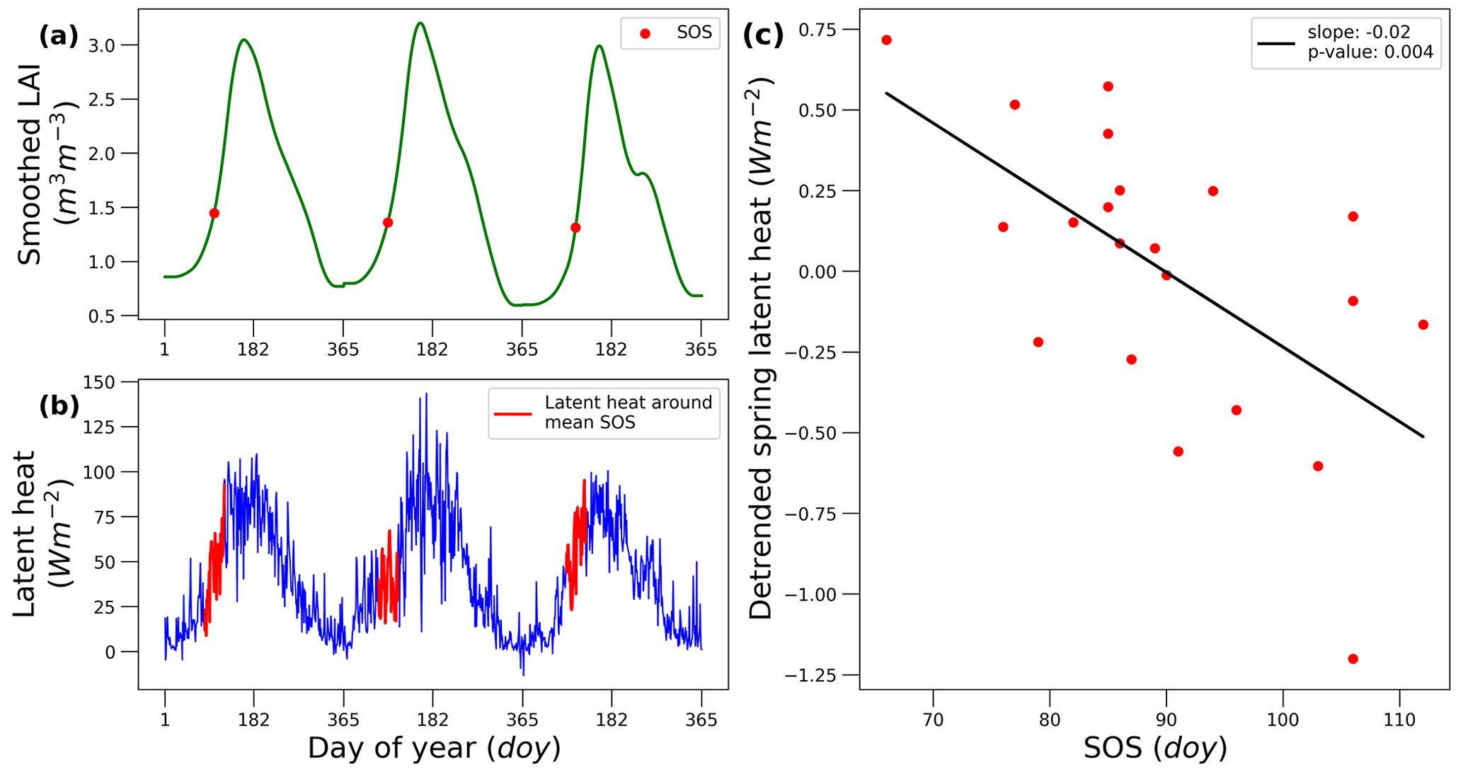
Figure 1 Example of the sensitivity calculation of latent heat to SOS between 2001 and 2003 at 52° N and 11° E. (a) SOS derived from smoothed MODIS-GLASS LAI data by using the EasyPhenology (Panwar, 2023) approach and threshold 0.3. (b) Selection of spring latent heat (±20 d around the mean SOS) calculated from ERA5 evaporation data. (c) The sensitivity and significance is derived from the linear regression between the detrended mean annual spring latent heat and the annual SOS date.

3 Results and Discussion

We first assess how phenological shifts modulate surface albedo, which controls the fraction of incoming solar radiation absorbed at the land surface and thereby constrains the energy supply for turbulent heat fluxes. We then examine the sensitivities of latent and sensible heat fluxes and their combined effect on evaporative fraction, before discussing potential implications for land surface temperature. We augment our sensitivity analyses with partial correlation estimates. Prior to discussing details in the sections to come, some general statements can be made: Overall, the partial correlation patterns broadly reproduce the spatial patterns and dominant trend directions identified in the sensitivity analysis, however, some regions no longer exhibit significant or weaker linkages. This reduction is most pronounced for H and EF at high latitudes and particularly for SOS-related responses. In contrast, the patterns of albedo sensitivities are well reproduced by the partial correlations and EOS-related relationships show more coherent agreement between correlation and sensitivity analyses. Together this suggests that, particularly in spring, temperature and other co-varying factors contribute to the spatial variability and magnitude of sensitivities of turbulent fluxes, whereas EOS-related responses are more directly attributable to phenological timing. We note, however, that ERA5 latent heat, sensible heat, and skin temperature are all outputs of the same integrated land-surface–atmosphere model, which may complicate interpretation of ERA5-based partial correlations due to potential residual within-product dependencies. However, the composite maps contain the average results across multiple data sources, including the FLUXCOM and GLEAM datasets, which provide additional independent support for the partial correlations of the turbulent fluxes.

3.1 Albedo

Spring albedo shows widespread significant positive sensitivities to SOS over boreal and Arctic regions. For example, sensitivities reach up to ${\mathrm{0.004}}_{\mathrm{0.002}}^{\mathrm{0.006}}$ (unitless; median with 25th and 75th percentiles) in deciduous needleleaf forests from the ERA5 albedo dataset, indicating that an earlier SOS is associated with declining albedo (Fig. 2a, b). Strong positive sensitivities also occur in evergreen needleleaf forests and tundra, as well as in high mountain regions such as the European Alps, Pyrenees, Caucasus, Altai, and Rocky Mountains. In contrast, mid-latitude regions in Europe, Central and Eastern Asia, and eastern North America exhibit negative sensitivities, implying increasing albedo with earlier SOS.

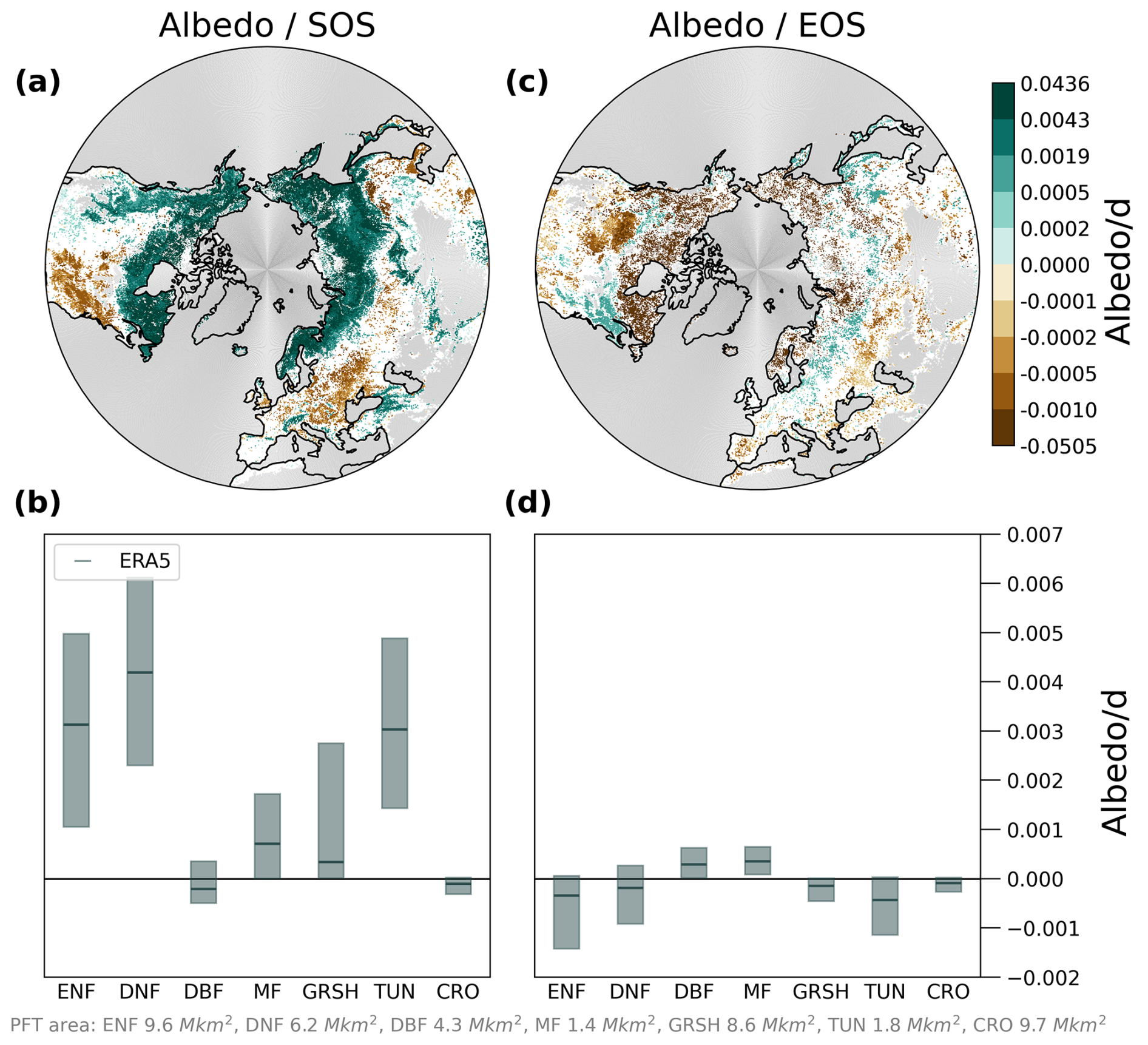
Figure 2 Sensitivity of spring and autumn albedo to SOS (a–b) and EOS (c–d), respectively. Sensitivities are for the period 2001 to 2021. (a, c) Linear regression significant (p value ≤0.05) detrended slope of spring albedo with SOS (a) and autumn albedo with EOS (c) from the ERA5 dataset. Water, urban and built-up areas, permanent snow and ice, barren and sparsely vegetated areas, and areas with LAI <0.5 are masked gray and non-significant slopes are masked white. (b, d) Statistical distributions of slopes for each land cover. Boxplots show the median (line), 25th and 75th percentiles (box). ENF evergreen needleleaf forest, DNF deciduous needleleaf forest, DBF deciduous broadleaf forest, MF mixed forest, GRSH grass and shrubland, TUN tundra, CRO croplands.

Positive sensitivities in tundra and boreal forests are likely driven by spring green-up masking residual snow cover, thereby reducing surface albedo. Conversely, negative sensitivities in croplands and deciduous broadleaf forests likely reflect canopy development shielding darker soils during spring green-up, particularly under moist soil conditions (Richardson et al., 2013). In agricultural systems, increased albedo may additionally arise from earlier sowing of brighter crops (Menzel et al., 2020).

Partial correlation analyses confirm these regional sensitivities of spring albedo to SOS, although areas of positive relationships are less spatially continuous and correlation magnitudes are more uniform across regions than the corresponding regression slopes (Fig. A2a).

Autumn albedo sensitivities to EOS are generally weaker and less spatially coherent than in spring. High-latitude regions, particularly tundra and evergreen needleleaf forests, tend to show negative sensitivities, indicating decreasing albedo with delayed EOS, likely due to prolonged canopy cover over bright soils or early snow. Deciduous broadleaf and mixed forests show on average positive sensitivities, consistent with extended leaf cover over relatively dark soils. Partial correlations reproduce these autumn patterns with similar spatial coverage and trend directions, although correlations at high latitudes are not markedly stronger than at lower latitudes (Fig. A2b).

As stated above, phenological shifts toward an earlier SOS result in the largest albedo responses in evergreen needleleaf forest, deciduous needleleaf forest, and tundra, with changes of 0.003–0.004 in albedo per day of SOS advance (Fig. 2b). To give a sense of magnitude in the context of the surface energy balance, we present a first-order estimate, based on the following assumptions: (i) the multi-decadal ERA5-Land average downward shortwave radiation for May–June over northern lands (>30° N) is used as the representative flux value; (ii) this downward flux is treated as approximately time-invariant over the study period; and (iii) the albedo change is assumed to act uniformly across the analysis domain. Using the ERA5-Land average of 257±18 W m⁻² (the uncertainty is the spatially aggregated standard deviation of daily estimates for those months; May–June marks the SOS period, see Fig. A2a), the albedo change converts to a change in reflected shortwave energy. An albedo decrease of 0.003–0.004 per day thus corresponds to a reduction in reflected shortwave of about 0.77±0.05 to 1.01±0.07 $\mathrm{W}{\mathrm{m}}^{-\mathrm{2}}{\mathrm{d}}^{-\mathrm{1}}$ for the regions considered. This additional shortwave absorption at the surface increases available energy potentially fueling turbulent heat fluxes, which we discuss next.

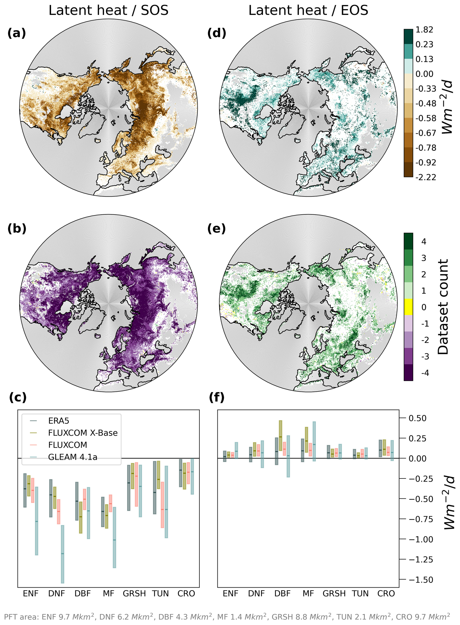
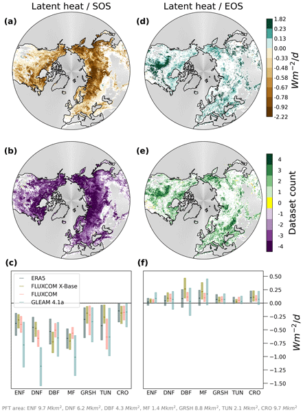
Figure 3 Sensitivity of spring and autumn latent heat (LE) to SOS (a–c) and EOS (d–f), respectively. Sensitivities are for the period 2001 to 2021. (a, d) Average significant (p value ≤0.05) linear regression detrended slope of spring LE with SOS (a) and autumn LE with EOS (d) across datasets with the same majority slope direction. Water, urban and built-up areas, permanent snow and ice, barren and sparsely vegetated areas, and areas with LAI <0.5 are masked gray, and non-significant slopes are masked white in all maps. (b, e) Significant slope direction count (negative or positive) of all four datasets. (c, f) Statistical distributions of slopes for each dataset and land cover. Boxplots show the median (line), 25th and 75th percentiles (box). ENF evergreen needleleaf forest, DNF deciduous needleleaf forest, DBF deciduous broadleaf forest, MF mixed forest, GRSH grass and shrubland, TUN tundra, CRO croplands.

3.2 Latent heat fluxes

Spring latent heat fluxes exhibit widespread significant negative sensitivities to SOS (Fig. 3a–c), ranging from $-{\mathrm{0.68}}_{-\mathrm{0.85}}^{-\mathrm{0.52}}$ $\mathrm{W}{\mathrm{m}}^{-\mathrm{2}}{\mathrm{d}}^{-\mathrm{1}}$ in mixed forests to $-{\mathrm{0.15}}_{-\mathrm{0.35}}^{-\mathrm{0.03}}$ $\mathrm{W}{\mathrm{m}}^{-\mathrm{2}}{\mathrm{d}}^{-\mathrm{1}}$ in croplands. This indicates enhanced latent heat fluxes with earlier SOS. Sensitivities are negative across all vegetation types and strongest over forests. The four datasets show consistent large-scale patterns across most northern lands.

These results align with increased energy supply through shortwave radiation absorption (Sect. 3.1) and reported evidence that increasing vegetation cover during spring enhances transpiration (Schwartz, 1996; Panwar et al., 2020), primarily regulated by photosynthetic activity via stomatal conductance (Richardson et al., 2013). Partial correlations support this relationship, showing overall significant negative associations between spring LE and SOS, albeit with reduced spatial coverage compared to the sensitivity analysis (Fig. A3a, b).

Autumn latent heat generally exhibits positive sensitivities to EOS, reaching up to ${\mathrm{0.14}}_{\mathrm{0.004}}^{\mathrm{0.329}}$ $\mathrm{W}{\mathrm{m}}^{-\mathrm{2}}{\mathrm{d}}^{-\mathrm{1}}$ in mixed forests (Fig. 3d–f), indicating increasing LE with delayed EOS. Compared to SOS, EOS sensitivities are weaker, more spatially heterogeneous, and less consistent across datasets. In particular, GLEAM shows regionally negative sensitivities in forested areas. Partial correlations reveal strong associations in regions such as Central North America and eastern Europe and indicate comparable or slightly stronger LE–EOS correlations than LE–SOS correlations (Fig. A3c, d).

This variability likely reflects constraints imposed by soil moisture availability and seasonal meteorological conditions. While delayed EOS may enhance transpiration, limited water availability towards the end of the growing season can decouple phenology from evaporation (Migliavacca et al., 2012; Richardson et al., 2013). An additional and potentially active confounding factor is that an earlier SOS may progressively deplete soil moisture reserves through extended transpiration and canopy interception over summer, directly suppressing autumn latent heat flux independently of EOS timing. Where soil moisture is limiting at the start of autumn, reduced stomatal conductance and transpiration would dampen the expected positive EOS–LE response, or even reverse it. This is consistent with the weaker and more spatially heterogeneous EOS–LE sensitivities we report compared to SOS, and with the regionally negative EOS–LE sensitivities found in some datasets – particularly GLEAM, where explicit soil moisture constraints on evaporation are represented. The negative sensitivities that occur in some regions support the hypothesis of limited water reserves with an elongation of the growing season (Buermann et al., 2018), but the location and abundance varies between the different datasets.

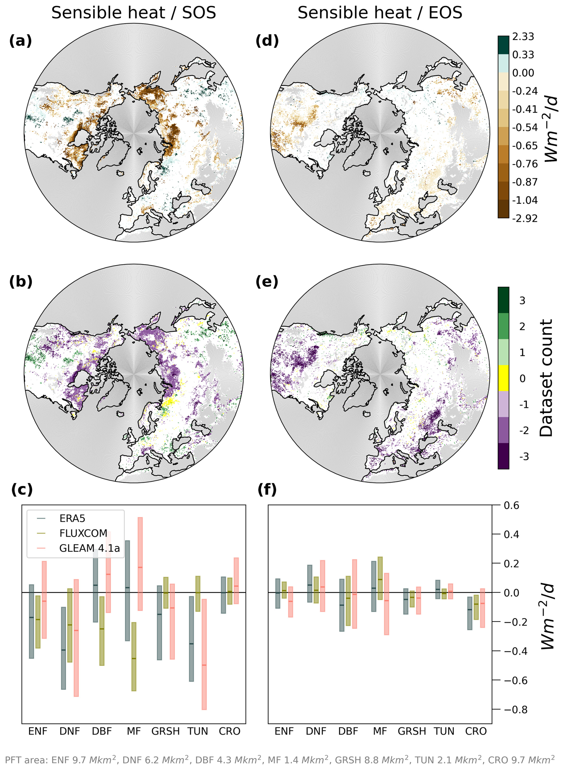
Figure 4 Sensitivity of spring and autumn sensible heat (H) to SOS (a–c) and EOS (d–f), respectively. Sensitivities are for the period 2001 to 2021. (a, d) Average significant (p value ≤0.05) linear regression detrended slope of spring H with SOS (a) and autumn H with EOS (d) across datasets with the same majority slope direction. Water, urban and built-up areas, permanent snow and ice, barren and sparsely vegetated areas, and areas with LAI <0.5 are masked gray, and non-significant slopes are masked white in all maps. (b, e) Significant slope direction count (negative or positive) of all three datasets. (c, f) Statistical distributions of slopes for each dataset and land cover. Boxplots show the median (line), 25th and 75th percentiles (box). ENF evergreen needleleaf forest, DNF deciduous needleleaf forest, DBF deciduous broadleaf forest, MF mixed forest, GRSH grass and shrubland, TUN tundra, CRO croplands.

3.3 Sensible heat fluxes

Sensitivities of sensible heat to SOS and EOS show no coherent large-scale pattern for northern lands and exhibit strong regional variability and dataset divergence (Fig. 4). However, smaller regions do exhibit coherent responses: spring H sensitivities to SOS are significantly negative across parts of northern Eurasia, particularly Siberia (Fig. 4a). Deciduous needleleaf forests show sensitivities of $-{\mathrm{0.24}}_{-\mathrm{0.643}}^{\mathrm{0.005}}$ $\mathrm{W}{\mathrm{m}}^{-\mathrm{2}}{\mathrm{d}}^{-\mathrm{1}}$, whereas other vegetation types display weaker and often mixed responses. Differences between datasets are especially pronounced in temperate and boreal Eurasia, with FLUXCOM generally indicating more negative or neutral sensitivities than ERA5 and GLEAM.

Partial correlations reveal little spatially extensive significant association between H and SOS, showing only weak tendencies towards negative correlations at some high latitude regions and positive correlations at some low latitude regions (Fig. A4a, b), reinforcing the absence of a robust spring signal.

Autumn sensible heat sensitivities to EOS are spatially mixed but show greater agreement between datasets than in spring (Fig. 4e, f). Central and south-eastern North America consistently exhibit negative sensitivities (e.g. $-{\mathrm{0.08}}_{-\mathrm{0.24}}^{-\mathrm{0.02}}$ $\mathrm{W}{\mathrm{m}}^{-\mathrm{2}}{\mathrm{d}}^{-\mathrm{1}}$ in croplands). Partial correlations coincide with these regions of significant sensitivities, again mainly showing negative relationships in mid- and lower-latitude regions (Fig. A4c, d).

Overall, these results show substantial uncertainty in how phenological shifts affect sensible heat. However, in high northern latitudes – particularly for deciduous and evergreen needleleaf forests and tundra (Fig. 4a, c) – a pattern of increased sensible heat flux with earlier SOS is emerging, mirroring the increase in latent heat flux (see Sect. 3.2). With both turbulent heat fluxes increasing, additional energy is required, consistent with the larger shortwave absorption from reduced albedo (Sect. 3.1). In the next section we examine how the partitioning of turbulent heat fluxes, expressed as the evaporative fraction (EF), responds to phenological shifts.

3.4 Evaporative fraction and surface temperature

Generally, sensitivities of EF integrate concurrent changes in LE and H (Fig. 5). Spring EF largely mirrors LE patterns, showing widespread negative sensitivities to SOS, indicating increasing EF with earlier SOS (Fig. 5a). Sensitivities reach $-{\mathrm{0.002}}_{-\mathrm{0.0048}}^{\mathrm{0.0012}}$ in deciduous needleleaf forests (Fig. 5c). ERA5 and GLEAM exhibit substantially larger variability than FLUXCOM-derived estimates. Regional positive sensitivities occur in Central Asia and the western United States, but datasets show limited agreement in these areas. Partial correlations reproduce the dominant spatial patterns but with reduced coverage, particularly at high latitudes (Fig. A5).

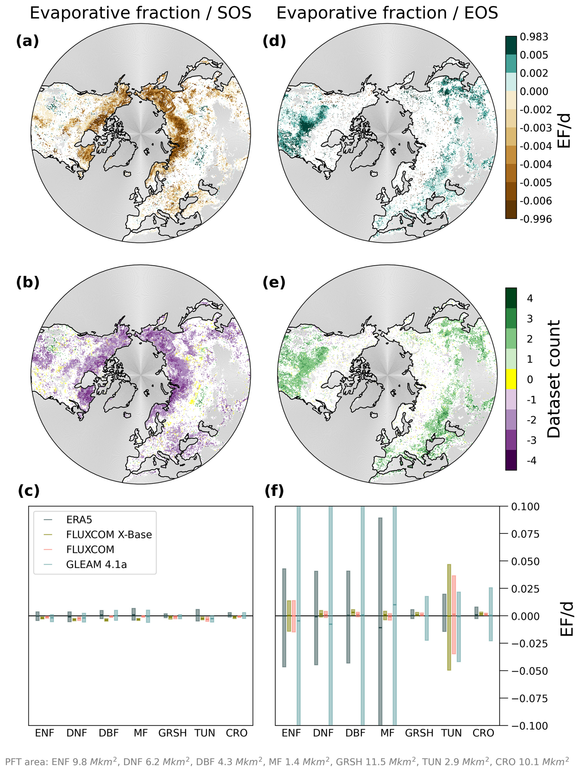
Figure 5 Sensitivity of spring and autumn evaporative fraction (EF) to SOS (a–c) and EOS (d–f), respectively. Sensitivities are for the period 2001 to 2021. (a, d) Average significant (p value ≤0.05) linear regression detrended slope of spring EF with SOS (a) and autumn EF with EOS (d) across datasets with the same majority slope direction. Water, urban and built-up areas, permanent snow and ice, barren and sparsely vegetated areas, and areas with LAI <0.5 are masked gray, and non-significant slopes are masked white in all maps. (b, e) Significant slope direction count (negative or positive) of all four datasets. (c, f) Statistical distributions of slopes for each dataset and land cover. Boxplots show the median (line), 25th and 75th percentiles (box). ENF evergreen needleleaf forest, DNF deciduous needleleaf forest, DBF deciduous broadleaf forest, MF mixed forest, GRSH grass and shrubland, TUN tundra, CRO croplands.

Autumn EF generally increases with delayed EOS in temperate regions (Fig. 5d), reaching ${\mathrm{0.0011}}_{-\mathrm{0.0008}}^{\mathrm{0.0054}}$ in croplands. Agreement among datasets is found across large parts of the Mediterranean, Central and Eastern Asia, and North America. In boreal and Arctic regions, however, EF sensitivities are spatially heterogeneous and datasets frequently disagree, particularly in boreal forests and tundra where ERA5 and GLEAM show much larger magnitudes than FLUXCOM. These discrepancies indicate substantial uncertainty in EF responses to phenological shifts. The potential confounding by SOS-driven soil moisture depletion (see Sect. 3.2) may likewise partially explain the dataset disagreement and spatial heterogeneity in autumn EF sensitivities: where soil moisture is limiting, suppressed transpiration reduces EF independently of EOS timing, masking or reversing the expected positive EOS–EF relationship.

Since rising surface temperature – primarily driven by increased downwelling longwave radiation from greenhouse gases over the long term – is the key driver of phenological changes, one cannot estimate the effect of phenological changes back on surface temperature. In other words, surface temperature both influences and responds to phenology through coupled energy-balance processes, and observational analyses cannot disentangle these feedbacks or provide quantitative causal attribution. Thus, we can only speculate about emerging effects linked to phenology based on observations.

The sensitivity analyses reveal negative associations between spring surface temperature and SOS and predominantly positive associations between autumn temperature and EOS (Fig. 6), consistent with earlier SOS and delayed EOS under warmer conditions. Warmer conditions also drive increases in both H and LE; however, the concurrent increases in EF suggest enhanced latent cooling, pointing toward a potential negative phenological feedback on surface warming. The negative partial correlations of LE and EF with SOS (Figs. A3 and A5) – i.e., statistically controlling for the effect of surface temperature – lend support to phenology-driven latent cooling. We therefore hypothesize that phenological shifts may partially offset GHG-induced surface warming through enhanced evaporation.

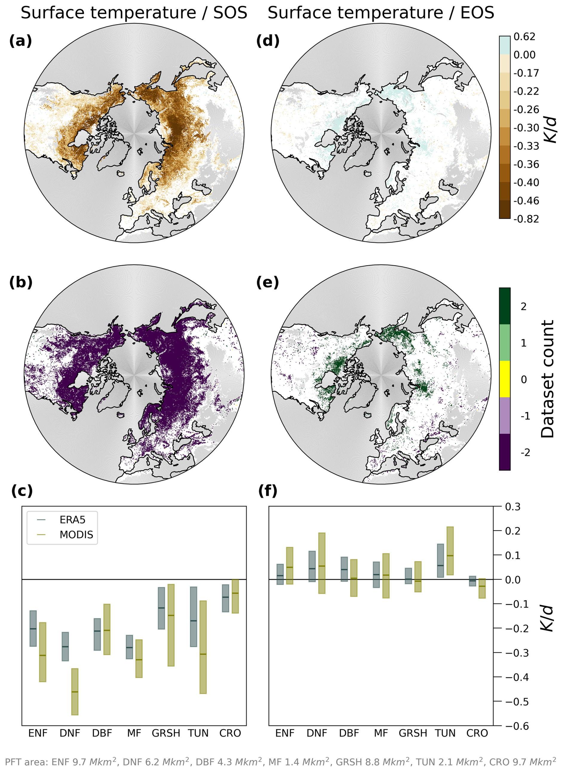
Figure 6 Relationship of spring and autumn surface temperature to SOS (a–c) and EOS (d–f), respectively. Sensitivities are for the period 2001 to 2021. (a, d) Average significant (p value ≤0.05) linear regression detrended slope of spring T with SOS (a) and autumn T with EOS (d) across datasets with the same majority slope direction. Water, urban and built-up areas, permanent snow and ice, barren and sparsely vegetated areas, and areas with LAI <0.5 are masked gray, and non-significant slopes are masked white in all maps. (b, e) Significant slope direction count (negative or positive) of all two datasets. (c, f) Statistical distributions of slopes for each dataset and land cover. Boxplots show the median (line), 25th and 75th percentiles (box). ENF evergreen needleleaf forest, DNF deciduous needleleaf forest, DBF deciduous broadleaf forest, MF mixed forest, GRSH grass and shrubland, TUN tundra, CRO croplands.

3.5 Robustness of Surface Energy Balance Sensitivities Across Plant Functional Types

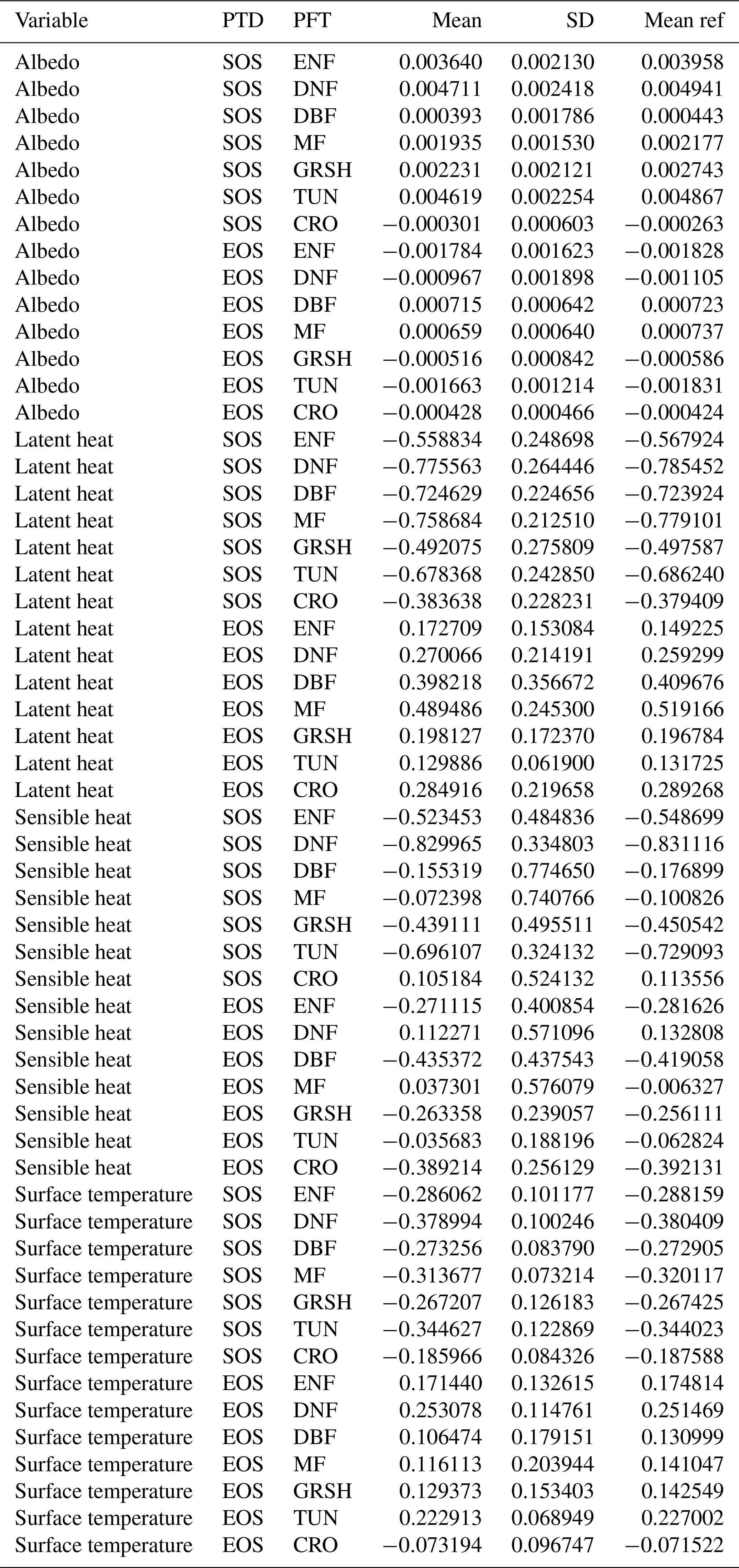
Overall, the estimated sensitivities are robust to the choice of analysis settings. Across all surface energy balance variables and PFTs, the spatially averaged reference slopes (30 % threshold, ±20 d window) generally fall near the centre of the distributions obtained from the alternative threshold and window width settings, and within one standard deviation of their mean (Figs. 7, A6, Table A1). The sign of the response is preserved in almost all cases; apparent sign changes occur only for H in MF, where mean sensitivities are close to zero across all settings and therefore do not represent a reversal of a meaningful trend.

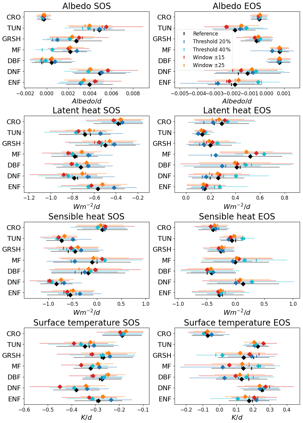
Figure 7 Statistical distribution of significant sensitivity slopes for the different analysis settings by plant functional type and surface energy balance variable. The reference analysis uses a 30 % threshold of the annual maximum LAI and a temporal window of ±20 d around the mean SOS/EOS. The alternative settings include a 20 % threshold, a 40 % threshold, a ±15 d window, and a ±25 d window. In each sensitivity analysis, only one parameter (threshold or window width) is varied, while the other is kept identical to the reference analysis. Results are shown for albedo, latent heat, sensible heat, and surface temperature. For each variable and plant functional type, the mean (diamond), median (vertical line), and standard deviation (horizontal error bar) of the significant sensitivity slopes are shown for evergreen needleleaf forest (ENF), deciduous needleleaf forest (DNF), deciduous broadleaf forest (DBF), mixed forest (MF), grass and shrubland (GRSH), tundra (TUN), and croplands (CRO).

The reference setting tends to produce slightly larger absolute slopes than the mean across all alternative settings and is most pronounced for SOS, where the ratio of larger to smaller reference slopes is roughly 8:1. EOS sensitivities show the greatest absolute deviation from the cross-settings mean, though the differences remain within the reported standard deviation.

Among the surface energy balance variables, sensible heat is the most robust: mean slopes and standard deviations are consistent across settings and PFTs. By contrast, autumn surface temperature shows the greatest sensitivity to the choice of analysis setting, with somewhat broader inter-setting distributions, particularly for GRSH and MF.

Among PFTs, mixed forest exhibits the highest sensitivity to the choice of settings, with large inter-setting variability. Croplands, in contrast, show the most compact and consistent distributions across all settings, with comparatively small sensitivities. This pattern that may partly reflect the managed nature of agricultural ecosystems.

Overall, the variability in sensitivities across PFTs and surface energy balance variables substantially exceeds the variability introduced by the tested methodological choices, suggesting that the observed responses primarily reflect underlying ecosystem characteristics rather than the specific choice of threshold or window width.

4 Conclusions

Our multi-datasets analyses show that an earlier start of season (SOS) is consistently associated with enhanced latent heat flux across northern extratropical ecosystems, while delayed end of season (EOS) exhibits a similar but weaker and more spatially heterogeneous effect. The results suggest that increased latent heat associated with observed SOS/EOS shifts may promote evaporative cooling, implying a potential negative feedback on surface warming. Independent modelling evidence shows that earlier SOS enhances evaporative cooling across northern vegetated regions (Lian et al., 2022), and large-scale observational analyses demonstrate that LAI increases reduce the Bowen ratio through enhanced transpiration (Forzieri et al., 2020), both consistent with the LAI/phenology-driven latent cooling feedback reported here. A companion paper currently under review with overlapping authorship provides a complementary mechanistic assessment of these feedbacks (Winkler et al., 2026). Across datasets, phenology-related shifts are found to influence the surface energy balance, although substantial regional and inter-dataset variability – particularly for sensible heat fluxes and evaporative fraction – indicates persistent uncertainties. These uncertainties call for improving the explicit representations of dynamic vegetation-controlled land surface dynamics, e.g., in the climate reanalysis efforts such as the successors of ECMWF's ERA5.

Two main limitations should be noted. First, satellite-based phenology primarily reflects canopy greenness dynamics and does not resolve underlying drivers such as climatic forcing, vegetation composition changes, land management, or non-phenological greening trends. Second, we do not explicitly account for interactions between concurrent SOS and EOS shifts; for example, an earlier SOS may increase the likelihood of summer soil moisture depletion, thereby influencing autumn energy balance responses.

Building on these findings, future work could pursue three complementary directions: (1) applying comparable sensitivity analyses to land surface models to assess latent heat responses and better constrain uncertainties in sensible heat and evaporative fraction; (2) using modelling frameworks to quantify legacy effects of SOS/EOS shifts and to separate climate-driven phenological changes from other drivers, improving attribution; and (3) integrating site-level observations of phenology and energy fluxes to better understand stand-scale mechanisms.

Overall, our results indicate that phenology-related changes in surface energy partitioning may contribute to dampen surface warming, although counteracting effects from albedo changes as part of the Arctic amplification mechanism need to be considered. Quantifying the magnitude and persistence of these feedbacks under continued climate change remains an important topic for future research.

Appendix A: Supporting Information

A1 Supplementary Figures

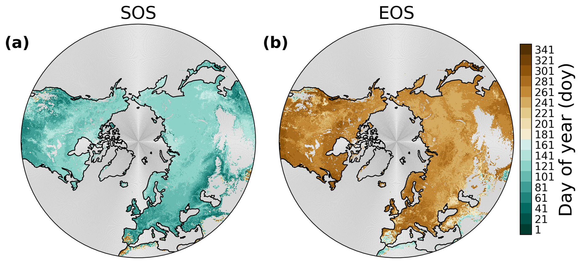
Figure A1 Spatial patterns of SOS (a) and EOS (b). The phenological transition dates are derived from smoothed MODIS-GLASS LAI data by using the EasyPhenology (Panwar, 2023) approach and threshold 0.3. Averaged phenological transition dates for the period 2001–2021 are displayed. Water, urban and built-up areas, permanent snow and ice, barren and sparsely vegetated areas, and areas with LAI <0.5 are masked gray.

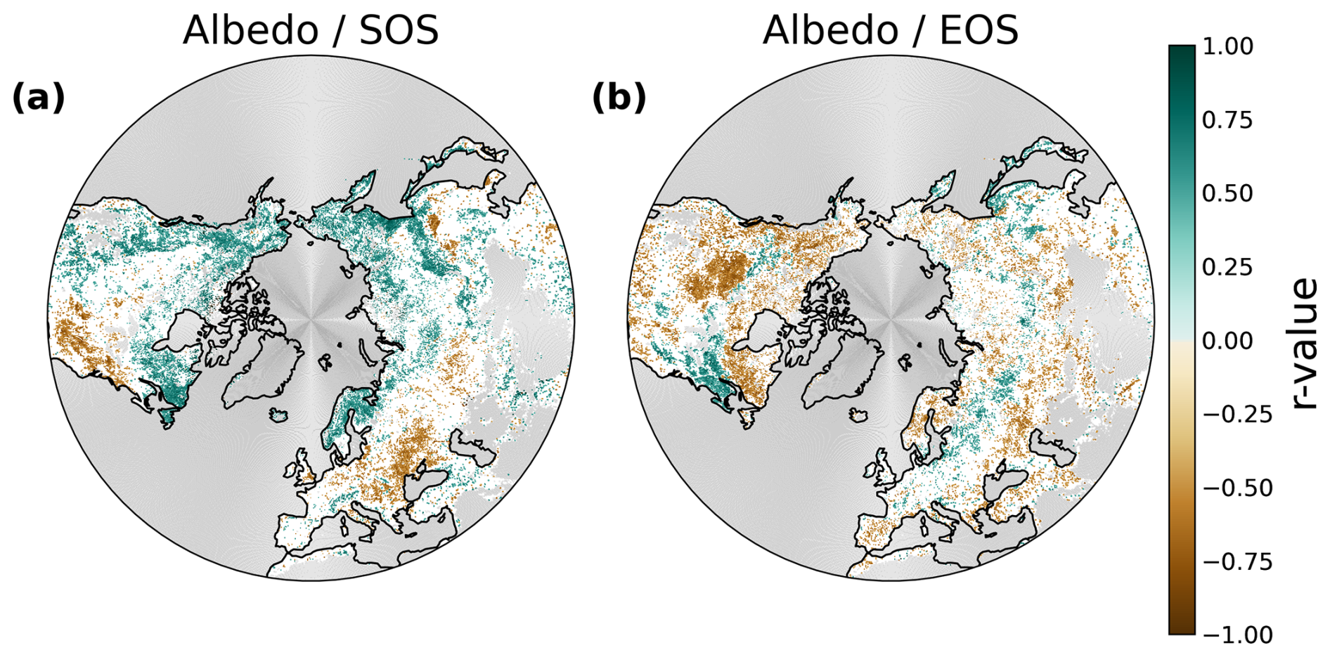
Figure A2 Spatial patterns of partial correlation between spring and autumn albedo with SOS and EOS, respectively, controlling for temperature. Significant (p value ≤0.05) relationship between detrended spring albedo with SOS (a) and autumn albedo with EOS (b), for the period 2001–2021. Water, urban and built-up areas, permanent snow and ice, barren and sparsely vegetated areas, and areas with LAI <0.5 are masked gray, and non-significant r values are masked white in the maps.

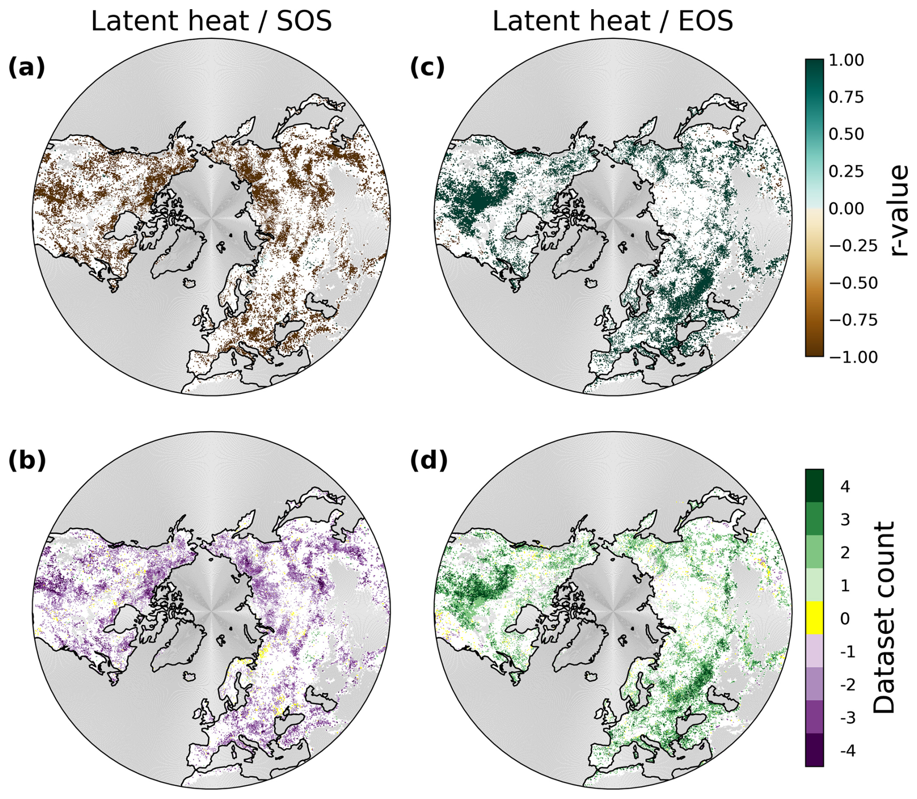
Figure A3 Spatial patterns of partial correlation between spring and autumn latent heat (LE) with SOS (a–b) and EOS (c–d), respectively, controlling for temperature. (a, c) Average significant (p value ≤0.05) relationship of detrended spring LE with SOS (a) and autumn LE with EOS (c) across datasets with the same majority r value direction, for the period 2001–2021. Water, urban and built-up areas, permanent snow and ice, barren and sparsely vegetated areas, and areas with LAI <0.5 are masked gray, and non-significant r values are masked white in all maps. (b, d) Significant r value direction count (negative or positive) of all four datasets.

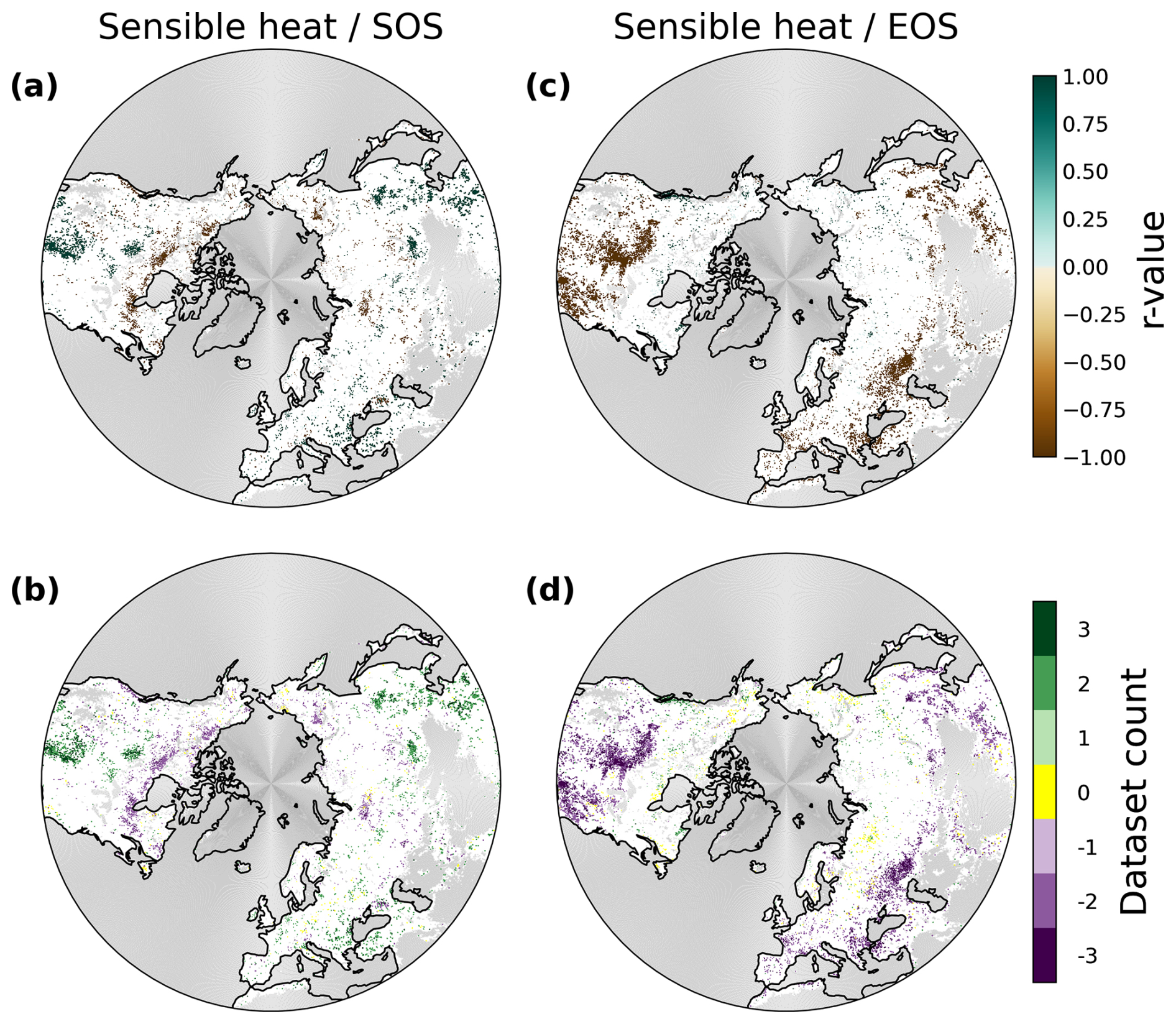
Figure A4 Spatial patterns of partial correlation between spring and autumn sensible heat (H) with SOS (a–b) and EOS (c–d), respectively, controlling for temperature. (a, c) Average significant (p value ≤0.05) relationship of detrended spring H with SOS (a) and autumn H with EOS (c) across datasets with the same majority r value direction, for the period 2001–2021. Water, urban and built-up areas, permanent snow and ice, barren and sparsely vegetated areas, and areas with LAI <0.5 are masked gray, and non-significant r values are masked white in all maps. (b, d) Significant r value direction count (negative or positive) of all three datasets.

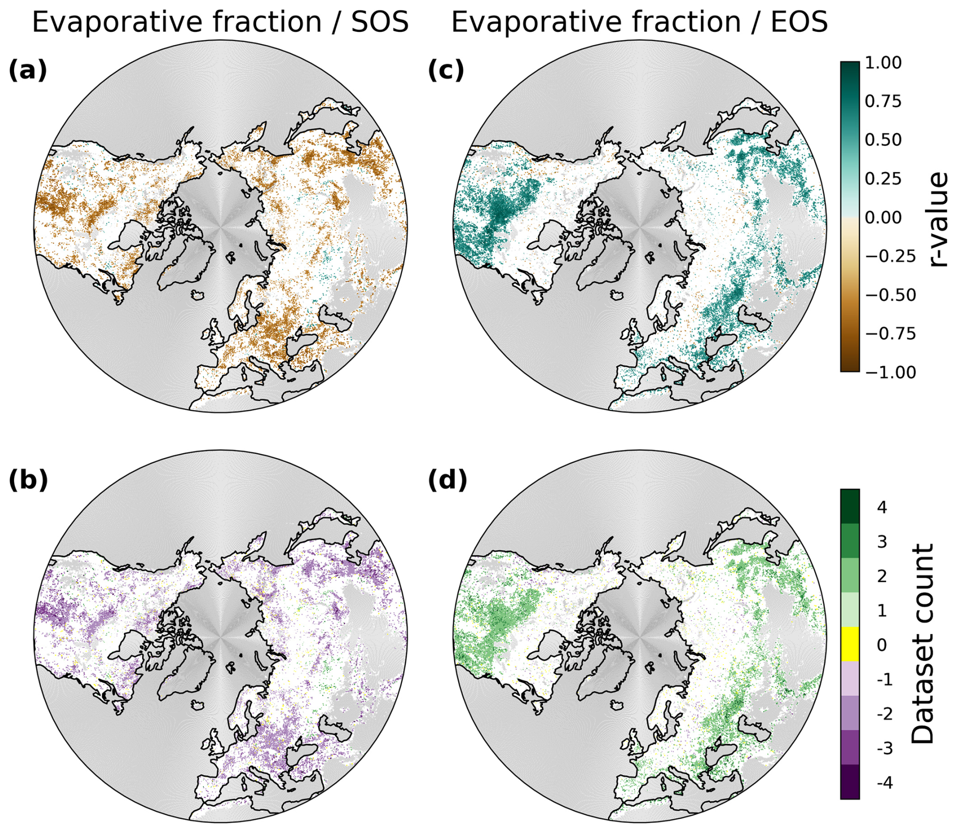
Figure A5 Spatial patterns of partial correlation between spring and autumn evaporative fraction (EF) with SOS (a–b) and EOS (c–d), respectively, controlling for temperature. (a, c) Average significant (p value ≤0.05) relationship of detrended spring EF with SOS (a) and autumn EF with EOS (c) across datasets with the same majority r value direction, for the period 2001–2021. Water, urban and built-up areas, permanent snow and ice, barren and sparsely vegetated areas, and areas with LAI <0.5 are masked gray, and non-significant r values are masked white in all maps. (b, d) Significant r value direction count (negative or positive) of all four datasets.

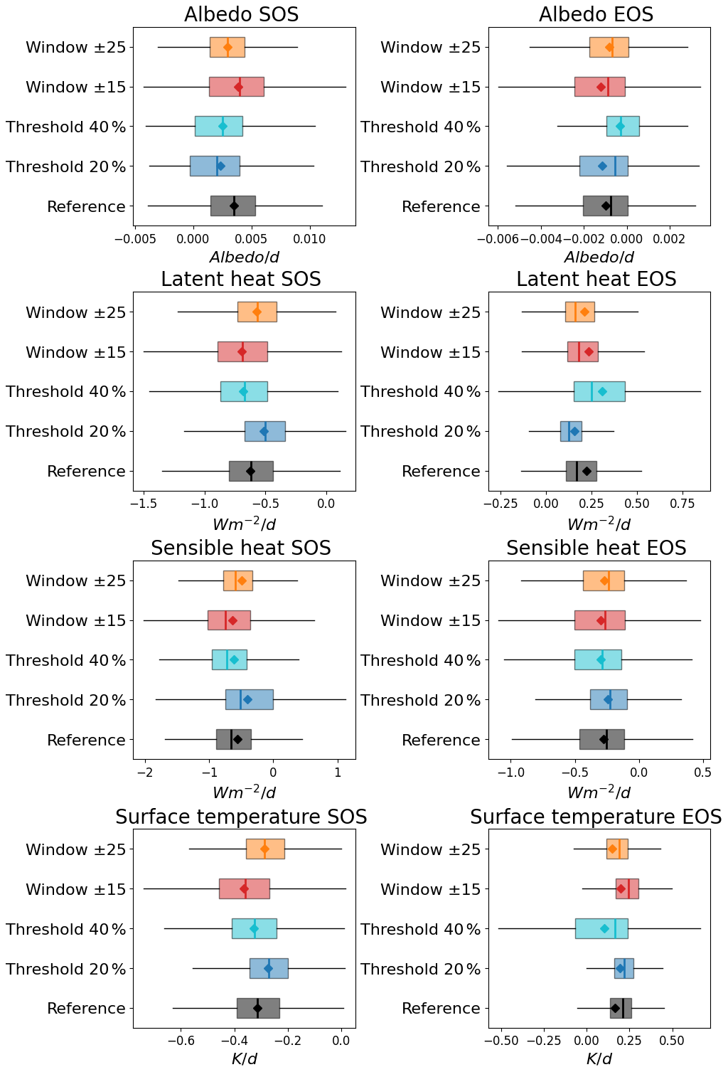
Figure A6 Statistical distribution of significant sensitivity slopes for the different analysis settings by surface energy balance variable. The reference analysis uses a 30 % threshold of the annual maximum LAI and a temporal window of ±20 d around the mean SOS/EOS. The alternative settings include a 20 % threshold, a 40 % threshold, a ±15 d window, and a ± 25 d window. In each sensitivity analysis, only one parameter (threshold or window width) is varied, while the other is kept identical to the reference analysis. Results are shown for the surface energy balance variables albedo, latent heat, sensible heat, and surface temperature. Box plots represent the distribution of significant sensitivity slopes (p value p≤0.05), with the box spanning the first and third quartiles (Q1–Q3), median (vertical line), mean (diamond), and whiskers (error bars).

A2 Supplementary Table

Table A1 Average significant sensitivities of surface energy balance variables (Albedo, LE, H, and surface temperature) to shifts in SOS and EOS across PFTs. The mean sensitivity (Mean) represents the average across all analysis settings (threshold 20 %, threshold 40 %, window width ±15 d, window width ±25 d, and the reference analysis). The spatially averaged sensitivities of the reference analysis (Mean ref) is based on a threshold of 30 % and window width of ±20 d, while the alternative analysis modify either threshold or window width. The average standard deviations across all analysis setting is reported as SD.