Technical note: a Recognition-assisted Camera for Automated Microscopy (RaCAM)

Automated microscopy workflows, including image acquisition, processing, and recognition using artificial intelligence (AI), are getting a growing interest from the scientific community in biogeosciences, as more and more research institutes are actively working on building datasets of images to train artificial convolutional neural networks (CNNs) to identify microscopic objects.

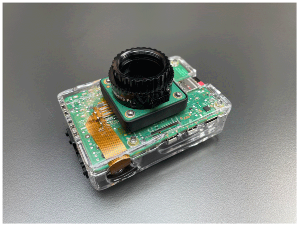
Here, we present a new, affordable, AI-assisted, and open-source Raspberry Pi-powered camera that can fit any microscope equipped with a regular C-mount (or CS-mount) camera thread. This camera is the first fully self-contained camera equipped with an integrated Single-Board Computer (Raspberry Pi 5) and high-resolution camera sensor (12.3 mp), attached together using a 3D-printable adaptor. Using two new open-source workflows written using the Python language and freely downloadable too, the camera is capable of performing automated microscopy using either an automated image segmentation workflow (RaCAM_IS software, including image acquisition, automated image processing, and object recognition using trained ResNet50 CNN models) or an object detection workflow (RaCAM_OD software, including image acquisition and automated still image/live stream object detection using YOLO models).

The camera is also adapted to on-field tasks such as core description, biostratigraphy or even palaeoenvironmental reconstructions based on microfossils census data or morphometry, as it can operate without the need for a spare computer and run directly on a power bank. Finally, since the automated microscopy workflows rely on images directly captured by the camera, applications can also be extended outside of the microscopy and micropaleontology research fields as any picture acquired with this device can virtually be processed.

1 Introduction

The past decades, and especially the last few years, have seen the development of artificial intelligence (AI) technology such as deep learning methods, applied to the training of convolutional neural networks (CNNs) to automatically recognise datasets of images. Rapidly, this technology has been used in the field of micropalaeontology to detect and recognise images of microscopic objects. Various groups of microfossils have been investigated so far using deep learning techniques, including coccoliths (Dollfus and Beaufort, 1999; Beaufort and Dollfus, 2004; Beaufort et al., 2026), foraminifera (Mitra et al., 2019; Hsiang et al., 2019; Marchant et al., 2020; Richmond et al., 2022; Govindankutty Menon et al., 2023; Piva et al., 2024; Tetard et al., 2026), pollen (Daood et al., 2018; Bourel et al., 2020; Gimenez et al., 2024; Sanhueza et al., 2026; Shi et al., 2026; Theuerkauf and Gillert, 2026), radiolaria (Itaki et al., 2020; Tetard et al., 2020, 2023; Carlsson et al., 2022, 2023; Mimura et al., 2024, 2025), or even diatoms (Zhang et al., 2023; Abdelmguid et al., 2026). Automated recognition, especially when integrated into a fully automated microscopy workflow, allows for fast analysis and counting of microscopic object images, as well as generation of morphometric data, some of which would not be possible without automated measurement (e.g. shape parameters such as circularity). These automated workflows allow one to save a substantial amount of time for microfossil counting, as several hundreds of specimens typically have to be counted over hundreds of samples, a task historically performed manually by an operator, also requiring substantial taxonomic knowledge.

This technology, at first requiring a high-performance computer, gradually became more and more accessible to regular machines over the past years. Several initiatives have recently emerged regarding affordable microscopy based on Raspberry Pi boards and camera modules (Raspberry Pi Ltd., Johnston and Cox (2017), that can be easily programmed for any need such as microfluidic applications, environmental monitoring of plankton, or even biological research to cite a few). Some initiatives focused on building a whole Raspberry Pi-assisted microscope from mass-produced parts that can be easily bought (Whittaker, 2020; Lynn, 2019), or 3D-printed (Grant et al., 2020; William, 2022, 2023), but few of these are actually key-in-hand solutions, as the software part usually relies on manual acquisition of images from a command line terminal and/or manual processing of these images (Webb, 2017; Nowosad, 2025), and none of them integrate an automated microscopy workflow software capable of performing automated recognition relying on trained CNNs. Schneidereit et al. (2017) also focused on building and automating a motorised stage that could be fitted on a microscope to automatically capture FOV images for entire microscope slides.

As development on Raspberry Pi boards using Python libraries and machine learning are becoming more and more accessible, and micro-computers and camera sensors cheaper and more powerful over time, automated tools and deep learning can now be directly used on such compact machines. We decided to develop a portable, affordable, and high-resolution solution that can fit most microscopes in laboratories or directly in the field and can perform whole automated microscopy workflows including image capture, processing, and object recognition: the Recognition-assisted Camera for Automated Microscopy (RaCAM). Automated microscopy workflows usually rely either on an image segmentation workflow (including field of view (FOV) image acquisition, segmentation, and recognition of individual object; e.g Marchant et al., 2020; Tetard et al., 2020; Beaufort et al., 2026), or object detection techniques (including FOV image acquisition and object detection and labelling directly performed on FOV images; (Lokteva et al., 2026; Beaufort et al., 2026)). Between image segmentation and object detection workflows, no approach should be directly considered superior to the other, as both were historically developed with different goals in mind. For example, depending on the investigated group of organisms, type of images (e.g. colour or greyscale), image resolution (high vs. low resolution), performance vs. time balance, need for further morphometric analysis on specimens, and deployment of the workflow, one approach might be more suitable than the other. This is why we decided to develop both approaches on the RaCAM camera through two independent software: RaCAM_IS for the automated image segmentation workflow and RaCAM_OD for the object detection workflow.

Such a low-cost and key-in-hand solution could be attractive for replacing aging camera units, or developing automated microscopy in emerging countries without sacrificing image quality, for example following MIT (Massachusetts Institute of Technology) involvement in low-cost and open-source, yet high-impact technology for science, education, and community development (e.g., MIT D-Lab (Hoffecker, 2018); MIT HEALS Collaborative developing low-cost diagnostics using AI for life sciences research: https://betterworld.mit.edu/mit-heals/, last access: 21 January 2026). Such initiatives highlight a commitment to reducing the economic barriers of high-cost scientific tools by providing “do-it-yourself” solutions to science. It can also be of significant interest for the deployment of analytical clusters (e.g., participative scientific project willing to equip a fleet of boats or ARGO floats (Wong et al., 2020); field water quality assessments using freshwater diatoms; scientific expedition where anyone can operate the microscope without the need for several taxonomic experts to be deployed; oil company working on many boreholes at once and needing a system that can handle a massive amount of microfossils and other microscopic objects to facilitate stratigraphic correlations (Martinsen et al., 2026)).

2 Material and methods

In the following sections, we will present and explain how to build the RaCAM camera, as well as how to install and use all required packages and software needed to operate both the RaCAM_IS and the RaCAM_OD software.

Table 1 Comparison between Raspberry Pi camera modules specifications.

2.1 Hardware: cameras

We recommend using either the Raspberry Pi HQ camera (https://www.raspberrypi.com/documentation/accessories/camera.html#hq-camera, last access: 2 November 2026; Sony IMX477 sensor with a built-in CMOS adaptor, compatible with most microscope mounts), AI camera (https://www.raspberrypi.com/documentation/accessories/ai-camera.html, last access: 2 November 2026; Sony IMX500 sensor, comes with a built-in AI chip), or camera module V2 (https://www.raspberrypi.com/documentation/accessories/camera.html#camera-module-2, last access: 2 November 2026; Sony IMX219 sensor, cheapest but lower resolution. We opted for the HQ camera (12.3 mp; physical pixel size of 1.55×1.55 µm) as it is delivered with a CMOS camera adapter, and no built-in lens, allowing for direct microscope image acquisition straight out of the box, without having to apply a lens shading correction to all acquired images when the factory lens is removed from its sensor. In case a camera module V2 or AI camera is used, the built-in lens has to be removed (easy for the AI camera, more difficult for the V2 camera has it is slightly glued), and a lens shading correction recalibration has to be performed to prevent discolouration of the acquired images after removing the factory lens for microscope use. As the AI camera sensor comes with a built-in AI chip, allowing for faster AI inference, it might also be a wise choice to develop and use neural networks through this sensor. The specifications for all camera sensors can be found in Table 1. Finally, as the camera sensor sizes are relatively small by comparison to regular DSLR cameras, the user might need to couple the camera with a 0.5× or 0.63× reduction lens adaptor to increase its captured field of view.

The camera module V3 (https://www.raspberrypi.com/documentation/accessories/camera.html#camera-module-3, last access: 2 November 2026; Sony IMX708 sensor), is also cheap and equipped with built-in motorised autofocus, but making the removal of the built-in lens a critical step (on top of disabling the motorised autofocus). Using this camera module V3 for our application is thus not recommended.

2.2 Hardware: board and accessories

To achieve the best possible performance in terms of acquisition speed/quality/processing of images, and to prevent compatibility issues between all camera parts, we recommend using at least a Raspberry Pi 5 8 GB board, an official fan module, an official 27 W USB-C power supply (providing up to 3 A at 5 V; or a power bank), and at least a 32 GB high-speed micro-SD card (including A2, U3, V30 specs; mandatory to ensure the board functions at a proper speed) or a NVMe M.2 SSD (2230 or 2242) and SSD adaptor.

2.3 Hardware: costs

Depending on configuration and specific purposes, one might need to choose a board with more RAM, or a different camera sensor, but the costs should remain low. Including the recommended Raspberry Pi 5 8 GB version board (∼ EUR 100; recommended retail prices vary from ∼ EUR 50 to ∼ EUR 150 for the 1 GB to the 16 GB versions), HQ camera module (∼ EUR 55), fan (∼ EUR 5) and high-speed microSD card (∼ EUR 10; or NVMe M.2 SSD (2230 or 2242) and SSD adaptor: ∼ EUR 40), the total for a micro-computer built-in RaCAM camera is about ∼ EUR 170 (∼ EUR 120 to ∼ EUR 250 depending on the board version).

On top of the RaCAM camera, the cost of an official Raspberry Pi screen (∼ EUR 120, USB-powered), micro-HDMI to HDMI cable (∼ EUR 6), keyboard (EUR 18), mouse (∼ EUR 8) and power supply (∼ EUR 13) add another EUR 165, for a total cost of ∼ EUR 340 for the full set-up. All software and packages presented in the next section needed to run the automated workflow are free. A bill of materials list is available as Supplement in Table S1 and is shown in Fig. A1.

2.4 Hardware: camera adaptors and cases

Using the Fusion360 3D-design software, 3D-printable (preferentially resin), Raspberry Pi 5-compatible board cases and camera module adaptors were sketched, designed (Figs. 1 and 2), printed, and are freely accessible as Supplement and at https://github.com/microfossil/particle-classification-onnx (last access: 2 November 2026). These 3D models (RaCAM_3D_files.zip © 2026 by Martin Tetard) are licensed under CC BY-NC-SA 4.0. To view a copy of this license, visit https://creativecommons.org/licenses/by-nc-sa/4.0/ (last access: 2 November 2026). This licence is allowing use, modification, and redistribution under the same terms, for personal purposes only as long as credit is given to the creator, and preventing any commercial use.

The camera module adaptors (for the HQ camera, AI camera module, and camera module V2) allow the camera module to be attached directly to a board case, using M2 screws and nuts. The AI camera module adaptor (and camera module V2) design includes a C-mount and CS-mount threaded version (actual usability largely depends on the 3D-printer, and on the print quality; resin SLA printing is recommended). This design also allows to glue a Ø 16 mm round cover-slip to act as a protective glass for the exposed sensor. A second 3D-printable version of the AI camera module (and camera module V2) adaptor to attach the camera to a common C-mount converter that can be bought on third-party websites is also included in the downloadable package.

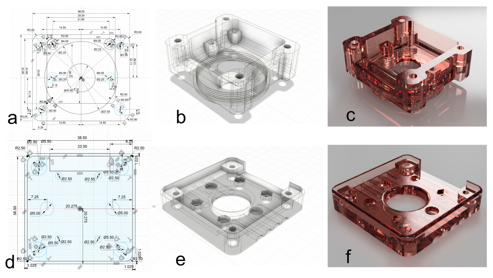
Figure 1 AI camera module (and camera module V2; a, b, c), and HQ camera (d, e, f) adaptors to fix the camera module to the board case designed using the Fusion360 3D-design software. (a) AI camera module adaptor schematic view. (b) AI camera module adaptor 3D view. (c) AI camera module adaptor rendering view. (d) HQ camera module adaptor schematic view. (e) HQ camera module adaptor 3D view. (f) HQ camera module adaptor rendering view.

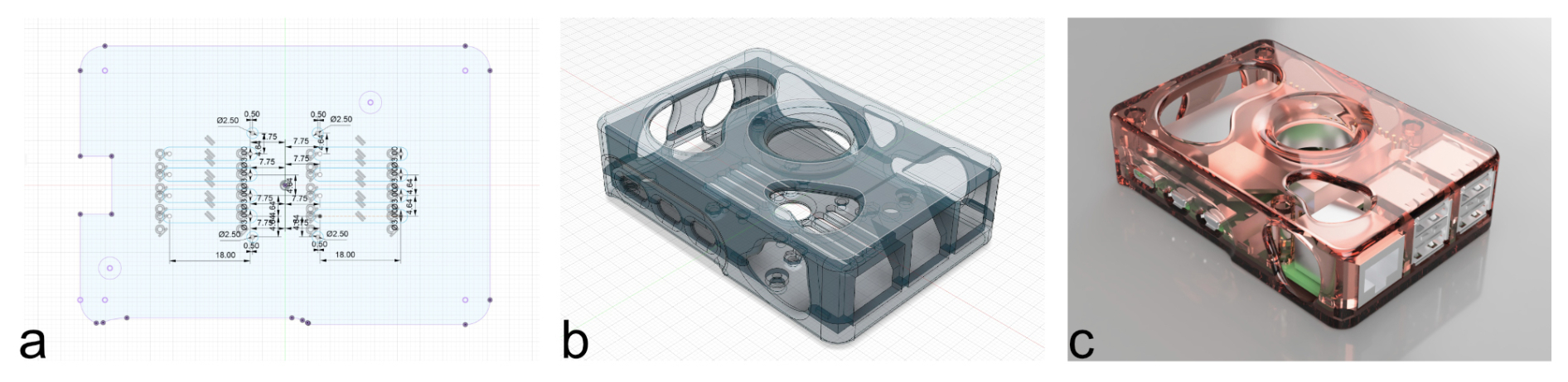
Figure 2 (a) Camera board case schematic view. (b) Camera board case 3D view. (c) Camera board case rendering view (designed using the Fusion360 3D-design software).

2.5 Hardware: assembling and mounting the camera

After 3D-printing one of the adaptor compatible with the camera module, both can be screwed together and fastened to the board case (see Fig. 3c) through the vent holes located under it, using M2 screws and nuts (4 × 12 mm for the HQ sensor adaptor + 4 × 5 mm washers; 4 × 8 mm + 4 × 10 mm for the AI and V2 sensor adaptor). The camera module ribbon cable can be plugged into the “CAM/DISP 0” port on the board, and the board can be secured to its case and closed using M2 screws and nuts (4 × 8 mm).

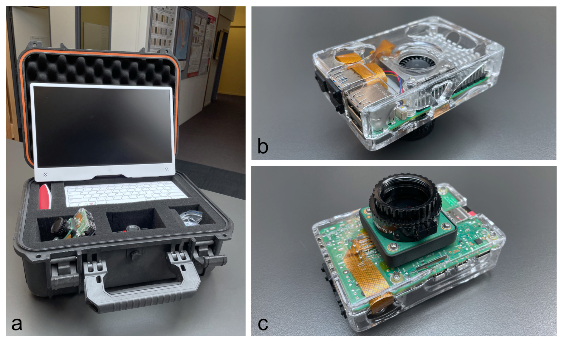
Figure 3 (a) RaCAM full set-up with transport and storage hard case. (b) Upper side view. (c) Lower side view.

Next, the camera can be mounted on the C-mount thread located on top of the microscope. It can then be connected to a USB-C power supply (or power bank), and connected to a screen using a micro-HDMI to HDMI cable. Finally, a keyboard and mouse can be connected to any USB-A ports on the main board.

2.6 Software: OS installation

Micro-computers/boards are usually key-in-hand and only require a micro-SD card or a NVMe M.2 SSD (2230 or 2242) loaded with the latest version of Raspberry OS (Linux distribution) to operate. A tutorial can be followed to easily format and install the last OS on a micro-SD card (https://www.raspberrypi.com/documentation/computers/getting-started.html#raspberry-pi-imager, last access: 2 November 2026), or on an NVMe M.2 SSD (https://www.raspberrypi.com/documentation/accessories/m2-hat-plus.html, last access: 2 November 2026). The current RaCAM_IS and RaCAM_OD software was developed in 2026 on Raspberry Pi OS (64 bit) running Debian version 13 (Trixie). These software are thus adapted for usage directly on the camera (Linux distribution), but could both potentially be easily adapted to run on any computer. If the reader wish to copy and paste command lines, we recommend doing it from the Installation_procedure_IS.txt and Installation_procedure_OD.txt files.

2.7 Software: downloading and installing Python packages

Some specific Python packages are required to run the RaCAM_IS and RaCAM_OD software, operating both automated microscopy workflows. To download and install them, open a new terminal window and then run:

• sudo apt update

• sudo apt upgrade

• sudo apt install python3-pip

• sudo apt install python3-tk

• sudo apt install python3-pil

• sudo apt install python3-pil.imagetk

2.8 Software: Image segmentation workflow

This section is dedicated to a step-by-step installation procedure of every software and package required to run the image segmentation workflow (segmentation of every individual particle present on an FOV image, and automated recognition of each of these particles using the RaCAM_IS software). These procedures are also detailed in the Installation_procedure_IS.txt file included in the RaCAM_IS_software.zip file (located in the /RaCAM_IS_files/ directory) and are available as Supplement and at: https://github.com/microfossil/particle-classification-onnx (last access: 2 November 2026).

The RaCAM_IS_software.zip (containing the RaCAM_IS software, ImageJ scripts, and miso-onnx library developed in this study) is protected under GNU GPLv.3 license (copyright © 2026 Martin Tetard). This license allows users to freely run, share, and modify software, while requiring that any modified versions be distributed under the same license terms, including the disclosure of source code.

2.8.1 Downloading and installing the RaCAM_IS software

The RaCAM_IS software is responsible for controlling the automated image segmentation workflow, from image acquisition, image processing and segmentation, to image recognition (Figs. 4 and 5), as well as batch processing of existing images and census data file generation.

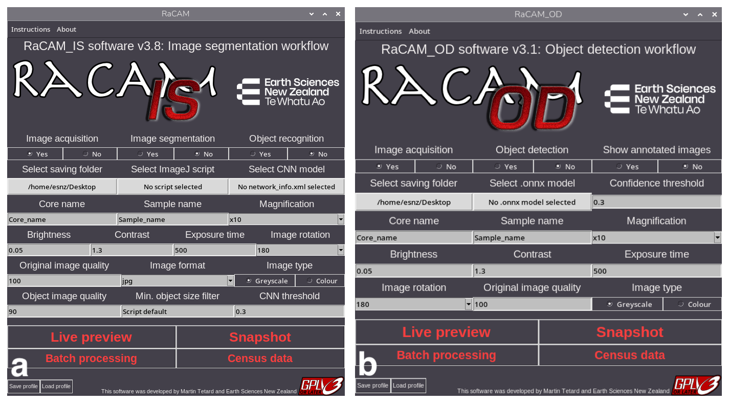
Figure 4 RaCAM_IS and RaCAM_OD software graphical user interfaces.

To check if your camera is detected and working properly, open a terminal window and run: rpicam-hello --timeout 0.

Then you can use “Ctrl+C” in the terminal window or simply the close button on the preview window to stop rpicam-hello.

For more information about the built-in camera software and the rpicam library, the reader is referred to https://www.raspberrypi.com/documentation/computers/camera_software.html (last access: 2 November 2026).

The RaCAM_IS software package (RaCAM_IS_software.zip) and the ResNet50_EoceneRadiolaria.zip (example images and CNN model) can be freely downloaded at: https://github.com/microfossil/particle-classification-onnx (last access: 2 November 2026) (and current version at the time of publication available as Supplement). It is an open-source software, using open-source packages and software. To install the RaCAM_IS software:

• Unzip the RaCAM_IS_software.zip file on the camera desktop and ensure that the RaCAM_IS file, and /RaCAM_IS_files/ and /RaCAM_IS_output/ folders are directly located on the desktop.

• Unzip the ResNet50_EoceneRadiolaria.zip file and place the ResNet50_EoceneRadiolaria folder in the /RaCAM_IS_files/CNN_models/ directory.

• Navigate to the /RaCAM_IS_files/ directory located on the desktop, right-click on the RaCAM_IS.py file, and select “Thonny” as default application to open this type of file.

• Open a file manager window, navigate to the “Edit” menu: “Preferences” and select “Don't ask option on launch of executable files” in the “General” tab.

• Right click on the RaCAM_IS file located on the desktop to open it with a text editor and update lines 3 (Exec=) and 4 (Icon=) by replacing <user> by your OS username (two times total), and save it. You should enter the username profile currently in use that can be found by looking at the path to the desktop directory (e.g. /home/<user>/Desktop/). You should now see the RaCAM_IS file icon as a RaCAM camera after a restart of the system.

• Double-click on it to start the RaCAM_IS software, you will be prompt to enter your username for updating paths for running the software. Again, you should enter the username profile currently in use, and that can be found by looking at the path to the desktop directory (e.g. /home/<user>/Desktop/.

• Once validated, the software should start successfully and you should be able to see the user interface (Fig. 4a). The RaCAM_IS software can now be closed as other software and packages are required before using it.

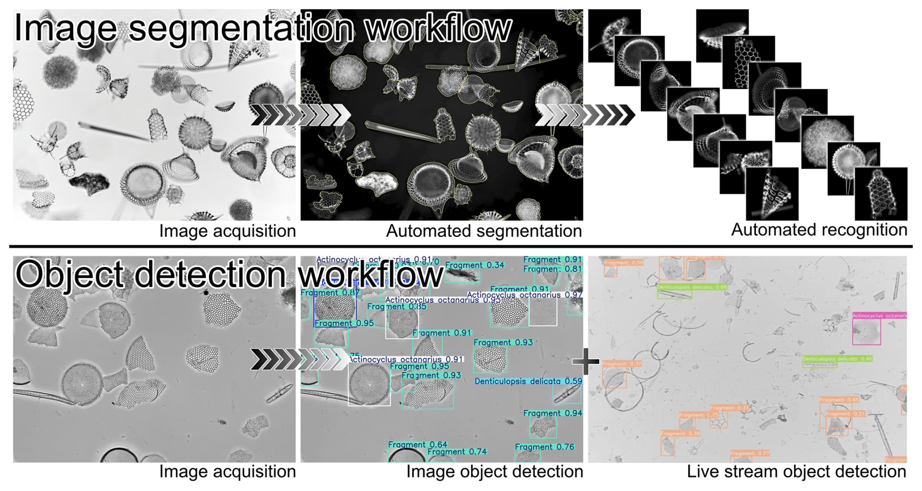
Figure 5 Different steps that can be performed individually or subsequently by the RaCAM_IS (image segmentation workflow) and RaCAM_OD (object detection workflow) software.

2.8.2 Download and installing ImageJ

ImageJ is an open-source software (Schneider et al., 2012) dedicated to image analysis and image processing. We use it in our workflow to automatically process the original FOVs that are captured during the acquisition step and segment every particle/microfossil into individual object images. To install it on the Raspberry Pi OS:

• Click on the top-left “Application menu bar” icon: “Preferences”: “Add/Remove software” and look for “Image processing program with a focus on microscopy images” and “Java library for ImageJ”. Select both of them then click “OK”.

• Start it in “Application menu bar” under “Education”, and close it.

• Navigate to /home/<user>/. Press “Ctrl+H” to show hidden files and folders.

• Go into the /home/<user>/.imagej/ directory.

• Copy the AutoRadio_RaCAMx10.ijm and Adjustable_Watershed.class files (located in /home/<user>/Desktop/RaCAM_IS_files/imagej_plugins/) into the /home/<user>/.imagej/macros/ and /home/<user>/.imagej/plugins/, respectively.

The AutoRadio_RaCAMx10.ijm script, originally published in Tetard et al. (2020) allows for batch processing of original FOVs. It is provided to allow the user to check that the workflow is working correctly by identifying an example set of images of marine plankton specimens (Eocene Radiolarian). It is specialised for segmentation of radiolarian specimens captured using a ×10 lens, but parameters can be easily modified for the segmentation of other microscopic objects, acquired at various magnification (and directly from the RaCAM_IS software interface).

2.8.3 Downloading and installing Miniconda3

Miniconda3 is an open-source environment manager that is used to handle specific Python packages and libraries installation through a virtual environment that cannot be used directly in the default OS environment. It is used in our workflow to automatically perform inference of segmented object images using pre-trained onnx models (based on ResNet50 CNNs) and the miso-onnx library (modified after (Marchant et al., 2020)). To install Miniconda3, open a new terminal window, and run:

• wget repo.anaconda.com

• wget https://repo.anaconda.com/miniconda/Miniconda3-latest-Linux-aarch64.sh

• bash ∼/Miniconda3-latest-Linux-aarch64.sh

Closely follow the instructions during Miniconda3 installation. Answer “Yes” to the license terms and install it in the default location (/home/<user>/miniconda3/), and answer “Yes” when asked to proceed to initialisation. After installing Miniconda 3, it is necessary to close the window to initialise it.

2.8.4 Install packages in the Miniconda3 environment

Next, to install packages in the Miniconda3 environment, open a new terminal window, run and accept main terms of service and proceed to installation:

• conda create -n miso-onnx python=3.11

• conda activate miso-onnx

• pip install opencv-python

• pip install numpy torch pillow onnxruntime

• pip install git+https://github.com/microfossil/particle-classification-onnx

Finally, check if the miso-onnx installation is successful by testing an onnx model inference using a CNN model pre-trained on Eocene radiolarian images (Tetard et al., 2020), and examples of radiolarian specimen images by running (after replacing the three <user> fields with your username):

• miso-onnx classify --network-info /home/<user>/Desktop/RaCAM_IS_files/CNN_models/ResNet50_EoceneRadiolaria/model_onnx/network_info.xml --images /home/<user>/Desktop/RaCAM_IS_files/CNN_models/ResNet50_EoceneRadiolaria/simple_test/unlabeled_images --output-csv /home/<user>/Desktop/RaCAM_IS_files/CNN_models/ResNet50_EoceneRadiolaria/simple_test/prediction_file/predictions.csv.

This operation should take a few seconds and should generate a .csv file located in /RaCAM_IS_files/CNN_models/ResNet50_EoceneRadiolaria/simple_test/prediction_file/. For more information about training an .onnx model for this workflow, the reader is referred to Marchant et al. (2020). For this example, all images are greyscale as per Tetard et al. (2020) and the individual input image size is reduced to 256×256 px² for memory saving purposes. The architecture chosen for CNN training of the example CNN model provided here for Eocene radiolaria is the ResNet50 with gain and cyclic layers, commonly used for microfossil identification (Mitra et al., 2019; Marchant et al., 2020; Bourel et al., 2020; Tetard et al., 2020; Carlsson et al., 2023; Tetard et al., 2023). This pre-trained model is focused on Eocene radiolaria, but the workflow can be applied to any microfossils observable under a transmitted or stereoscopic microscope. Using the ParticleTrieur software (Marchant et al., 2020) and documentation freely available at https://particle-classification.readthedocs.io/en/latest/installation.html (last access: 2 November 2026), the user can also train their own model, based on their own dataset of images and upload it to the RaCAM camera.

2.8.5 Using the RaCAM_IS software

This section is a step-by-step guide of every step required to use the image segmentation workflow (also available in Sect. S1 in the Supplement with images):

• When starting up the RaCAM_IS software, the user is presented with a graphical interface. In the first row of buttons, select the operation you wish to perform (“Image acquisition” and/or “Image segmentation” and/or “Object recognition”) by choosing “Yes” or “No” below each function (Fig. 4a).

• In the second row, select the corresponding saving folder/imagej script/CNN model network_info.xml file depending on the requested operations (e.g. you don't need to select an imagej script or CNN model if you only want to perform image acquisition; you can keep the saving folder by default: /home/<user>/Desktop/).

• In the third row, fill in information about the core, sample and magnification you are using (“Core_name”, “Sample_name”, and “Magnification” fields, which can also be used to account for any other kind of metadata if the acquisition does not follow a /Core/Sample/ structure). If the magnification is not in the drop-down list, you can directly write it (providing magnification has no impact on any data processing, it is just a metadata that will be written in the filename).

• In the fourth, fifth and sixth rows, adjust the parameters as you need such as brightness, contrast, exposure time, image (camera) rotation, image quality (% jpeg quality), image format (.jpg or .png), image type (8 bit greyscale or colour), segmented object image quality, minimum size for an object to be saved (px²), and finally the confidence threshold for a CNN to label an object image. More information about each parameter can be found in the “Instructions” tab directly in the software.

• The “Save profile” and “Load profile” can be used to save all these parameters before shutting down the software. Only one profile can be saved.

• Clicking on the “Live preview” button shows a livestream preview from your microscope so you can adjust the parameters, focal depth, and slide position before capturing and saving an image. The preview window must be closed before using any other function.

• Clicking on the “Snapshot” button captures an image and saves it in the “saving folder” (again, we recommend keeping the saving folder by default on the Desktop). The image will be saved in the /Desktop/RaCAM_IS_output/Image_acquisition/ directory following a /Core_name/Sample_name/Label/ path structure (Fig. A2) using the core name and sample name provided. If you also selected “Image segmentation”: “Yes”, and/or “Image recognition”: “Yes”, the corresponding images will also be saved in the /Desktop/RaCAM_IS_output/Image_processing/ and /Desktop/RaCAM_IS_output /Image_recognition/ directories, respectively.

• Clicking on the “Batch processing” button allows you to process an existing batch of image (either do segmentation on a batch of existing original FOV images, or identify a batch of segmented images, or both) by unselecting “Image_acquisition” and selecting “Image_processing” and/or “Image_recognition”: “Yes”, and providing an ImageJ script and/or CNN model. You will be asked to choose and enter a folder, which should be a “core” directory containing “sample” directories, containing images. For the recognition step, object images that will be labelled are those located in /RaCAM_IS_output/Temp/ temporary folder generated after an image segmentation job.

• Clicking the “Census data” button generates a census table (.csv file) containing taxa in columns and samples in rows, by scanning the /Label/ subdirectories of each /RaCAM_IS_output/Image_recognition/Core_name/Sample_name/ directory and compiling the number of images of each subdirectory (taxa abundance). When the “Census data” button is clicked, the user will be asked to choose a core directory, which must be selected and entered to successfully perform the census data generation.

2.9 Software: object detection workflow

This section is a step-by-step installation procedure of every software and package required to run the second available workflow, relying on object detection techniques (namely detection and recognition of particles of interest directly on the FOV image using the RaCAM_OD software and live detection). These procedures are also detailed in the Installation_procedure_OD.txt file included in the RaCAM_OD_software.zip file (located in the /RaCAM_OD_files/ directory) and are available as Supplement and at: https://github.com/microfossil/particle-classification-onnx (last access: 2 November 2026).

The RaCAM_OD_software.zip (containing the RaCAM_OD software) is protected under GNU GPLv.3 license (copyright © 2026 Martin Tetard). This license allows users to freely run, share, and modify software while requiring that any modified versions be distributed under the same license terms, including the disclosure of source code.

2.9.1 Downloading and installing the RaCAM_OD software

The RaCAM_OD software is responsible for controlling the automated object detection workflow, from image acquisition, object recognition, live detection (Figs. 4 and 5), as well as batch processing of existing images, and census data file generation.

To check if your camera is detected and working properly, open a new terminal window and run: rpicam-hello --timeout 0.

Then you can use “Ctrl+C” in the terminal window or simply the close button on the preview window to stop rpicam-hello.

For more information about the built-in camera software and the rpicam library, the reader is referred to https://www.raspberrypi.com/documentation/computers/camera_software.html (last access: 2 November 2026).

The RaCAM_OD software package (RaCAM_OD_software.zip) can be freely downloaded at: https://github.com/microfossil/particle-classification-onnx (last access: 2 November 2026) (and the current version at the time of publication available as Supplement). It is an open-source software, using open-source packages and software. To install the RaCAM_OD software:

• Unzip the Racam_OD_software.zip file on the camera desktop and ensure that the RaCAM_OD file, and /RaCAM_OD_files/ and /RaCAM_OD_output/ folders are directly located on the desktop.

• Navigate to the /RaCAM_OD_files/ directory located on the desktop, right-click on the RaCAM_OD.py file, and select “Thonny” as default application to open this type of file.

• Right click on the RaCAM_OD file located on the camera desktop and update lines 3 (Exec=) and 4 (Icon=) by replacing <user> by your OS username (three times total), and save it. You should enter the username profile currently in use and that can be found by looking at the path to the desktop directory (e.g. /home/<user>/Desktop/). You should now see the RaCAM_OD file icon as a RaCAM camera after a restart of your system.

• Double-click on it to start the RaCAM_OD software, you will be prompted to enter your username for updating paths for running the software. You should enter the username profile currently in use and that can be found by looking at the path to the desktop directory (e.g. /home/<user>/Desktop/).

• Once validated, the software should start successfully and you should be able to see the user interface (Fig. 4b). The RaCAM_OD software can now be closed as other software and packages are required before using it.

2.9.2 Create virtual environment, and install ultralytics and onnxruntime packages

• Open a new terminal window, then run and accept main terms of service if asked, and proceed to installation:

  • /usr/bin/python3 -m venv --system-site-packages yolo_OD

  • source yolo_OD/bin/activate

  • sudo apt update

  • sudo apt install python3-pip -y

  • pip install -U pip

  • pip install ultralytics[export]

  • pip install numpy picamera2 onnxruntime

  The ultralytics package install might be long, you can close the terminal window afterward.

  You can then run a test inference using the provided YOLO .onnx model:

• Copy the complete /Core_name/ folder from the /Desktop/RaCAM_OD_files/Test_inference/ directory into the /Desktop/RaCAM_OD_output/Image_acquisition/ directory.

• Double click on the RaCAM_OD software located on the desktop to start it.

• Select “Image acquisition”: “No”, “Object detection”: “Yes”, and “Show annotated images”: “Yes”, then select an .onnx model (located at /Desktop/RaCAM_OD_files/Exported_models/yolo11n1280_diatoms_test.onnx)

• Click on the “Batch processing” button that will prompt you to select and input core directory. Select and enter the /Desktop/RaCAM_OD_output/Image_acquisition/Core_name/ directory and click “Ok”.

• When batch processing is done, you should now see a labelled image containing annotated diatom taxa in the /Desktop/RaCAM_OD_output/Image_recognition/ directory, and a census file in the /Desktop/RaCAM_OD_output/Raw_census_data/ directory.

The example .onnx YOLO model provided here is a YOLO11n model with a 1280 px input image size. This pre-trained model is dedicated to a few marine diatoms taxa, but the workflow can handle any YOLO .onnx models (preferably nano, small, or medium) trained with an input image size of 640 to 1280 px (more than that makes inference more time consuming). Additional tutorials and information on how to build and label your training dataset, as well as training your own model, can be found at http://platform.ultralytics.com (last access: 2 November 2026).

2.9.3 Using the RaCAM_OD software

This section is a step-by-step guide of every step required to use the object detection workflow (also available in Sect. S1 with images):

• When starting up the RaCAM_OD software, the user is again presented with a graphical interface (Fig. 4b). In the first row of buttons, select the operation you wish to perform: “Image acquisition” and/or “Object detection” and/or “Show annotated images” (the latter will automatically open the annotated images after automated acquisition and object detection for manual control).

• In the second row, select the corresponding saving folder (default is /home/<user>/Desktop/) and/or a YOLO .onnx model file, and confidence threshold for object detection depending on the requested operations (e.g. you don't need to select an .onnx model if you only want to perform image acquisition; you can keep the saving folder by default).

• In the third row, the user should also fill in the “Core_name”, “Sample_name”, and “Magnification” fields. These can account for other metadata if you are not using a /Core_name/Sample_name/ path structure (Fig. A3). If the magnification is not in the drop-down list, you can directly write it (providing magnification has no impact on any data processing, it is just a metadata that will be written in the filename).

• In the fourth and fifth rows, adjust the image capture parameters as needed (brightness, contrast, exposure time, image (camera) rotation, image quality (% jpeg quality), image type (8 bit greyscale or colour) and neural network confidence threshold above which a label will be annotated). More information about each parameter can be found in the “Instructions” tab directly in the software.

• The “Save profile” and “Load profile” can be used to save all these parameters before shutting down the software. Only one profile can be saved.

• Clicking on the “Live preview” button shows a livestream preview from your microscope so that you can adjust the parameters, focal depth, and slide position before capturing and saving an image. The preview window must be closed before using any other function.

• Performing live stream object detection using the same .onnx YOLO model is also possible. By selecting “Image acquisition”: “No” and “Object detection”: “Yes”, the “Live preview” button will switch to “Live detection”, allowing you to perform automated live detection using the selected YOLO .onnx model. When you click on the “Live detection” button, a pop-up window will ask you for a target species: if you write a target class name exactly as learnt by the model, a snapshot will automatically be captured (saved in /RaCAM_OD_output/Live_detection/) by the software every time this target class is detected with a cool-down of 10 s, allowing one to manually drag the microscopic slide under the microscope and let the system capture images when needed. If you leave this field empty, no image will be automatically captured.

• Clicking on the “Snapshot” button captures an image and saves it in the “saving folder” (again, we recommend keeping the saving folder by default on the Desktop). The image will be saved in the /Desktop/RaCAM_OD_output/Image_acquisition/ directory following a /Core_name/Sample_name/ path structure (Fig. A3) and using the core name and sample name provided. If you also select “Object detection”: “Yes”, the corresponding images will be saved in the /Desktop/RaCAM_OD_output/Image_recognition/ directory, as well as an individual census file for each annotated image in the /RaCAM_OD_output/Raw_census_data/ directory.

• Clicking on the “Batch processing” button allows you to batch process an existing folder of FOV images for object detection. For this purpose, you need to select “No” for “Image acquisition” and “Yes” for “Object detection”, and click the “Batch processing” button after selecting a YOLO .onnx model. You will be asked to choose and enter a /Core_name/ directory located in /RaCAM_OD_output/Image_acquisition/. Annotated images will then be saved in /RaCAM_OD_output/Image_recognition/, as well as individual census files in /RaCAM_OD_output/Raw_census_data/.

• Clicking the “Census data” button will generate a .txt census table containing taxa in columns and samples in rows for all samples of the investigated core, by compiling the individual .txt files generated during the object detection step for each FOV image and located in the /Desktop/RaCAM_OD_output/Raw_census_data/ directory. When clicking the “Census data” button, the user will be asked to choose a core directory, which must be selected and entered to successfully perform the census data generation for a core directory

3 Results and Discussion

3.1 Overall camera performance

With a physical pixel size of 1.55 µm (for an effective pixel size of about 0.155 to 0.015 µm if used together with ×10 to ×100 magnification lenses, for example), the RaCAM camera resolution is comparable to an high-end camera for regular (i.e., stereoscopic or transmitted light) microscopy for a fraction of their price, As the camera is also able to directly perform image processing and recognition, and without any additional costs for any proprietary software, it is suitable for most purposes regarding image acquisition, processing or even recognition of microscopic objects using either the image segmentation or the object detection workflow. A direct comparison between the same FOV acquired on both the RaCAM camera (Sony IMX477 sensor) and an Axiocam 712 Mono Zeiss 12 mp camera (Sony IMX304 sensor) shows subtle to no difference, since most of the resolution is determined by the optical quality of the host microscope and lenses (Fig. 6). Of course, the difference in pricing is largely due to other features implemented in the high-end cameras (e.g., rolling shutter for the RaCAM vs. global shutter for most high-end cameras, much more advanced and expensive, but not mandatory for regular microscopy).

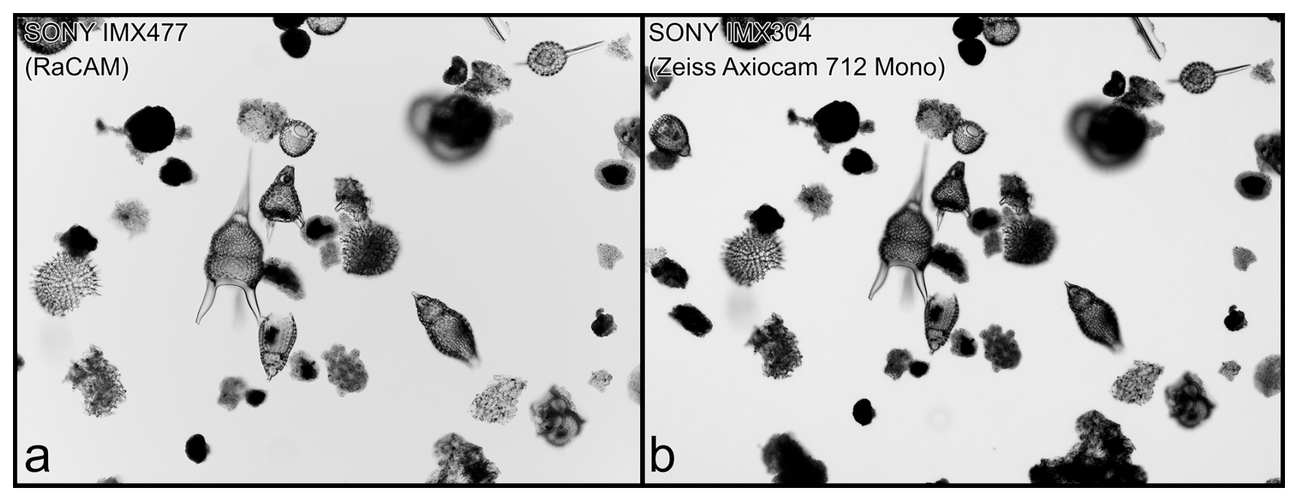
Figure 6 Image quality comparison for the same field of view (Eocene radiolarian fauna, sample IODP342-1407A-11H-CC) captured with the RaCAM camera (a), and a Zeiss 712 Mono camera (b).

The time required to perform the image segmentation workflow using the RaCAM_IS software for a single FOV image varies depending on the number of object images that are segmented and need to be identified and the board version (from 1 to 16 GB of RAM, the higher the better). Individually, the image capture step is almost instantaneous (excluding a 5 s delay, whose duration can however be increased or decreased, to perform a full-screen focal adjustment before the FOV image is actually captured). The image processing is about 4 s per FOV, and includes saving of all generated individual object images. Finally, time needed to perform image recognition is about 1–2 s per individual object image. For example, overall, the whole workflow would last for about 15 s (for 5 objects detected), 20–25 s (10 objects), 45 s (20 objects), and so on. Generating a census data file is almost instantaneous. As this workflow will save all the individual segmented images, it is more adapted to perform subsequent morphometric analysis, for example.

Regarding the object detection workflow using the RaCAM_OD software, the time required to perform acquisition and object detection on a single FOV image is very rapid. Again, the image capture step is almost instantaneous (excluding the 5 s delay to adjust the focal depth), and object detection step is about less than 1 s per FOV, including saving the original FOV image and a labelled copy of this image as well as individual census file. Generating a summary census data file is almost instantaneous. Live detection performance (in terms of frames per second, not accuracy) will greatly depend on available RAM, YOLO model variant (e.g. nano “n” will be faster but less accurate, extra large “x” will be more accurate but much slower; “n” to “m” recommended), as well as YOLO model image input size (e.g. 640 px will be faster but less accurate than 1280 px). As this workflow will directly annotate images with all objects detected, it is faster to run and operate than the RaCAM_IS software (about 1 s per FOV image vs. 1 s per individual object image). It is also easier and more straightforward to install and to run.

3.2 Comparison with other microscopy platform

In order to compare the RaCAM's ability to use a trained CNN model for image segmentation workflow against a regular automated microscopy platform (Zeiss AXIO Imager.M2 automated transmitted light microscope equipped with an Axiocam 712 Mono 12 mp camera, controlled with a Dell Precision 5820 computer, 64 go RAM and AMD Radeon Pro W6600 graphic card, routinely used at ESNZ), we decided to evaluate the overall recognition accuracy of the provided Eocene radiolarian CNN model (published in Tetard et al. (2023)). To do so, we performed the acquisition of the same new FOV images from two samples unknown to the CNN model (early (IODP342-1407A-11H-CC) and late Eocene (DSDP29-277-18-3-20cm)), on both the microscopy platform and the RaCAM mounted on an Olympus BX53 microscope. Both batches of FOV images were automatically segmented, and individual specimen images were identified using the same trained CNN model on both the Dell computer associated with the Zeiss microscope platform and directly on the RaCAM, respectively. The same 11 FOV images were acquired with both systems (due to subtle differences in final magnification, the total count of specimens varies between both; see Fig. 6). Of the 273 individual specimen images acquired with the microscope platform and automatically identified, 234 were correct (86 % overall accuracy). Of the 226 individual specimen images acquired and identified with the RaCAM, 192 were correct (85 % overall accuracy). Both systems thus perform very similarly, as expected by the overall accuracy predicted by the trained CNN itself (87.5 %; Tetard et al., 2023). This highlights that in this aspect, the RaCAM sensor and specifications can cope with high-end systems, as the recognition accuracy is mostly depending on the frozen model itself.

3.3 Field testing the camera

For an accurate and representative field testing of the camera, we decided to use it routinely during the third field season for the SWAIS2C programme (Sensitivity of the West Antarctic Ice Sheet to 2 degrees Celsius of warming), a six week field season on ice at Crary Ice Rise, located 700 km off Scott Base that aimed to recover a 200 m+ sediment core from below the ice sheet. The camera was mounted on a Nikon Alphaphot microscope for image capture of micropaleontological smear slide images for real-time microfossils assessment (diatoms, silicoflagellates, ebridian cysts) and biostratigraphic purposes during drilling operations.

For about two weeks, the camera was used continuously for 12–14 h a day as part of an upgraded biostratigraphic workflow, for live-monitoring of the drilling process by performing image acquisition of smear slides prepared from samples regularly recovered from every core section. When microfossils were present, about 20 FOV images per sample were acquired, and automatically processed using the RaCAM_IS software (image segmentation workflow; the object detection workflow was yet to be developed) to segment every particle (biogenic or not), which were then automatically labelled and saved using a CNN trained for inference of Quaternary to Pliocene Antarctic marine diatom images.

As the recovered samples were primarily Late to Early Miocene in age, most of the taxa imaged and labelled were not learnt by our trained CNN yet. However, most of the diatom specimens identified by the camera were assigned to morphologically and phylogenetically close taxa (e.g., species of the same genus such as Actinocyclus, Fragilariopsis and Thalassiosira species). As the CNN training (performed on another computer), and accuracy are independent from the camera itself, and only dependent on the image database it was trained on, we consider that no technical issue was encountered by the camera. Thus the automated image segmentation workflow using the RaCAM_IS software is fully operational. For future field work, new CNNs will be trained for other time intervals and loaded on the camera in order to cover a longer biostratigraphically significant time bin.

As the camera operates using a built-in micro-computer, allowing for other operations such as using spreadsheet, text document, web browser, and image acquisition, processing and recognition, it prevents the need for a separate computer (Fig. 7). With an average power consumption of about 3 W (about 6 W with full CPU load), the RaCAM is very energy efficient and can be operated in the field, or anywhere else, using a portable power bank (and together with the USB-powered Raspberry Pi screen).

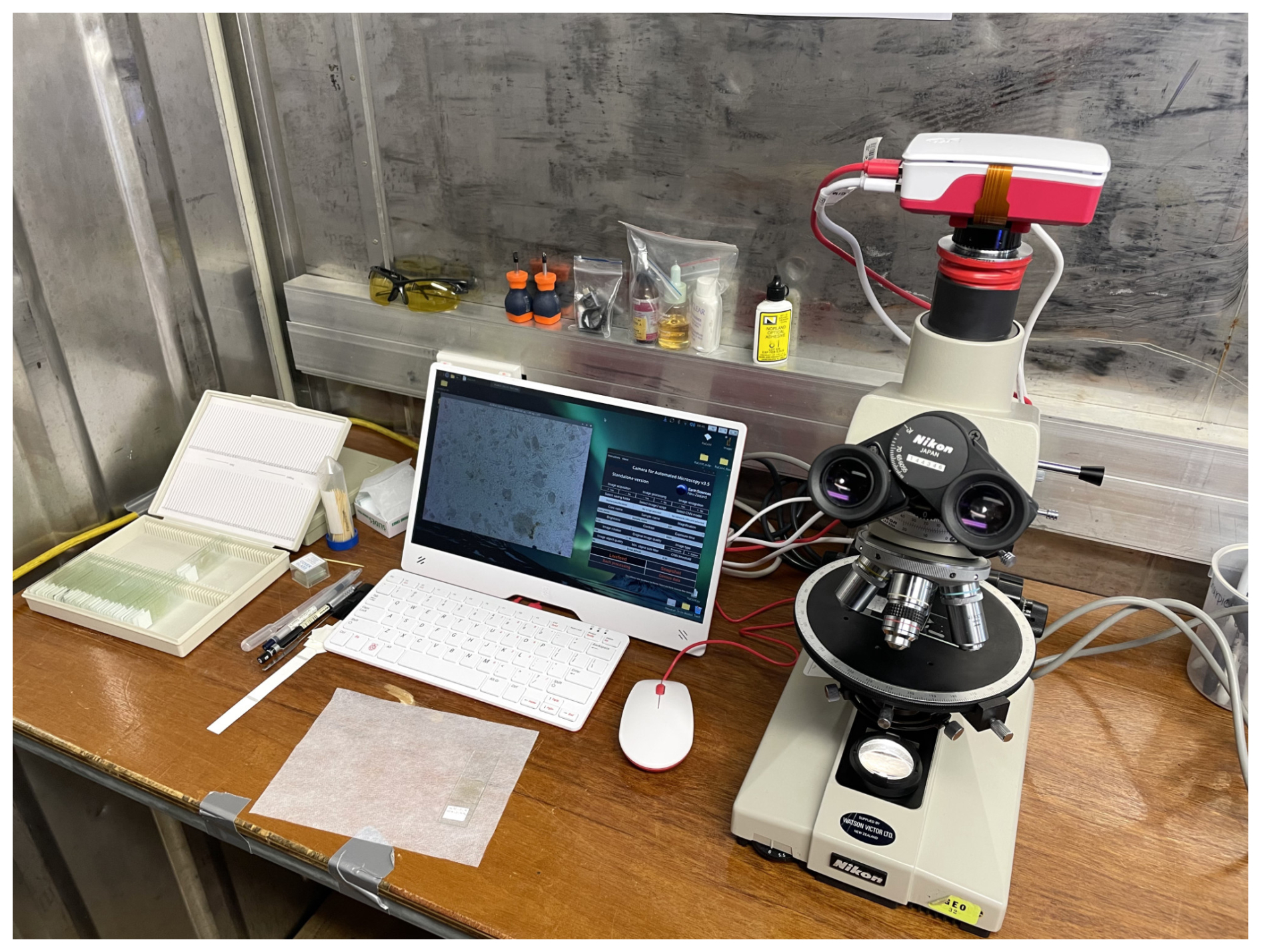
Figure 7 RaCAM camera mounted on a Nikon Alphaphot during the SWAIS2C 2025–2026 season, Crary Ice Rise.

4 Conclusions

We developed an affordable and fully automated camera that can be plugged into the C- or CS-mount thread of any microscope such as transmitted light or stereoscopic microscopes. At a cost of about ∼ EUR 120 to ∼ EUR 250 (depending on the board version), freely available OS, software and packages, and free guides to build it yourself, the RaCAM camera allows the user to perform two automated microscopy workflows, relying on image segmentation (RaCAM_IS software) and object detection (RaCAM_OD software) techniques, respectively.

Using the RaCAM_IS software, the user can perform image acquisition and/or automated image processing, and/or automated object recognition of segmented images using trained CNNs. Original, segmented, and classified images are saved. The software can also perform batch image segmentation and/or object recognition of existing images and generate summary census data files compiling taxa counts for every sample of a core. Using the RaCAM_OD software, the user can perform image acquisition and automated object detection directly on captured FOV images using common YOLO .onnx models. Original and annotated FOV images can be saved, as well as census data files. The software can also perform batch object detection for existing FOV images, and perform live stream object detection using the same YOLO .onnx model and automatically capture images when a target species is detected.

We emphasise that the object recognition accuracy, on both workflows, depends on the trained model performance (itself depending on the training dataset size, resolution, number of classes, morphological complexity and variability of the organisms of interest, to cite a few). Regarding image processing and recognition, the camera itself just acts as a micro-computer, using pre-trained models. We developed the two image segmentation and object detection workflow software around commonly used CNN models, such as the ones developed in Marchant et al. (2020) for ParticleTrieur, and YOLO models (now commonly used in micropaleontology), respectively, to allow people to re-use their existing models directly on the camera.

The installation and use procedure, RaCAM_IS and RaCAM_OD software, and 3D model files are available for free as Supplement and at: https://github.com/microfossil/particle-classification-onnx (last access: 2 November 2026). Our next step for the RaCAM project is to develop a motorised stage that would fit most microscopes and be directly controlled by the integrated computer board and coupled with the RaCAM automated microscopy workflows.

Appendix A

Figure A1 Schematic of all components required to assemble the RaCAM camera.

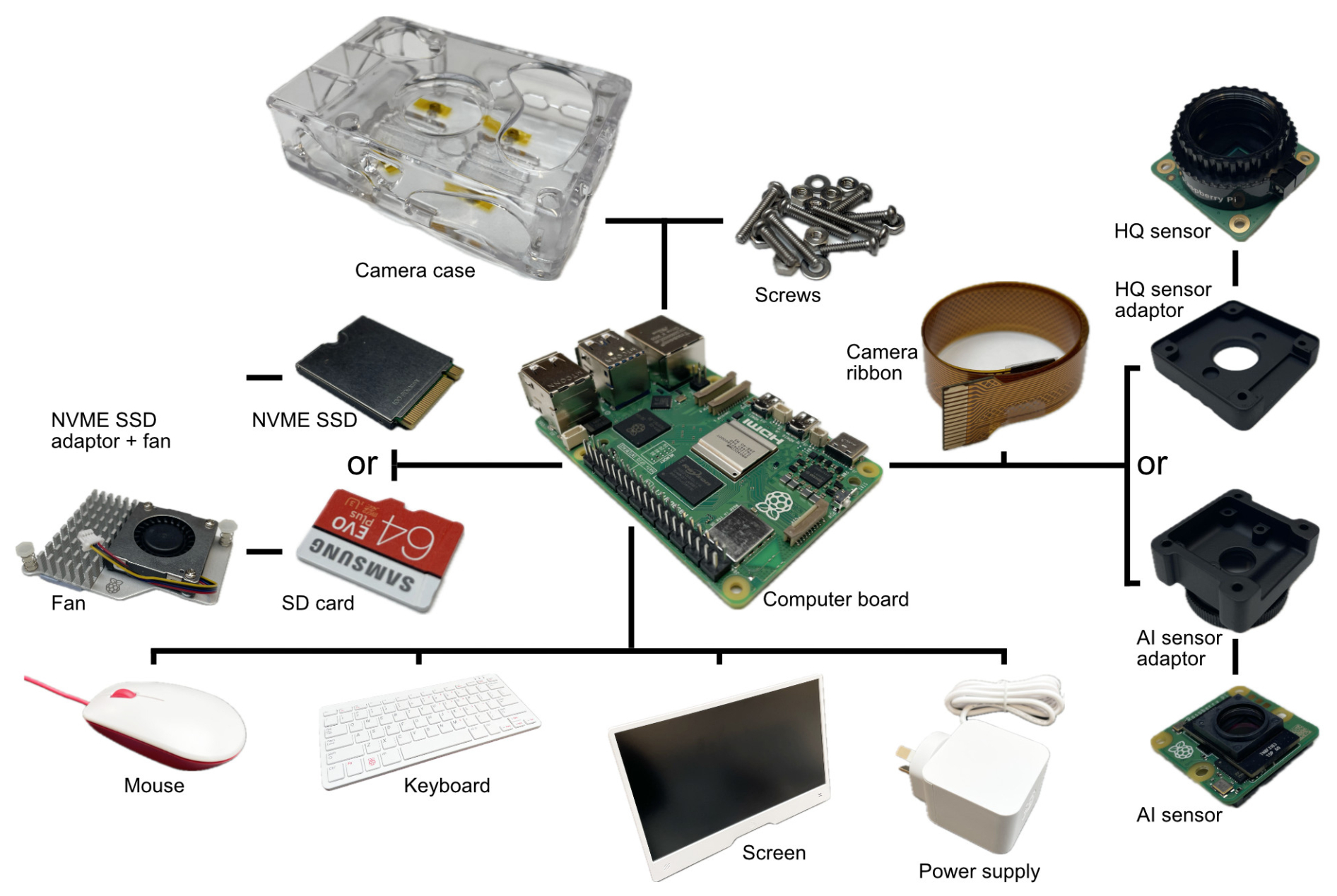
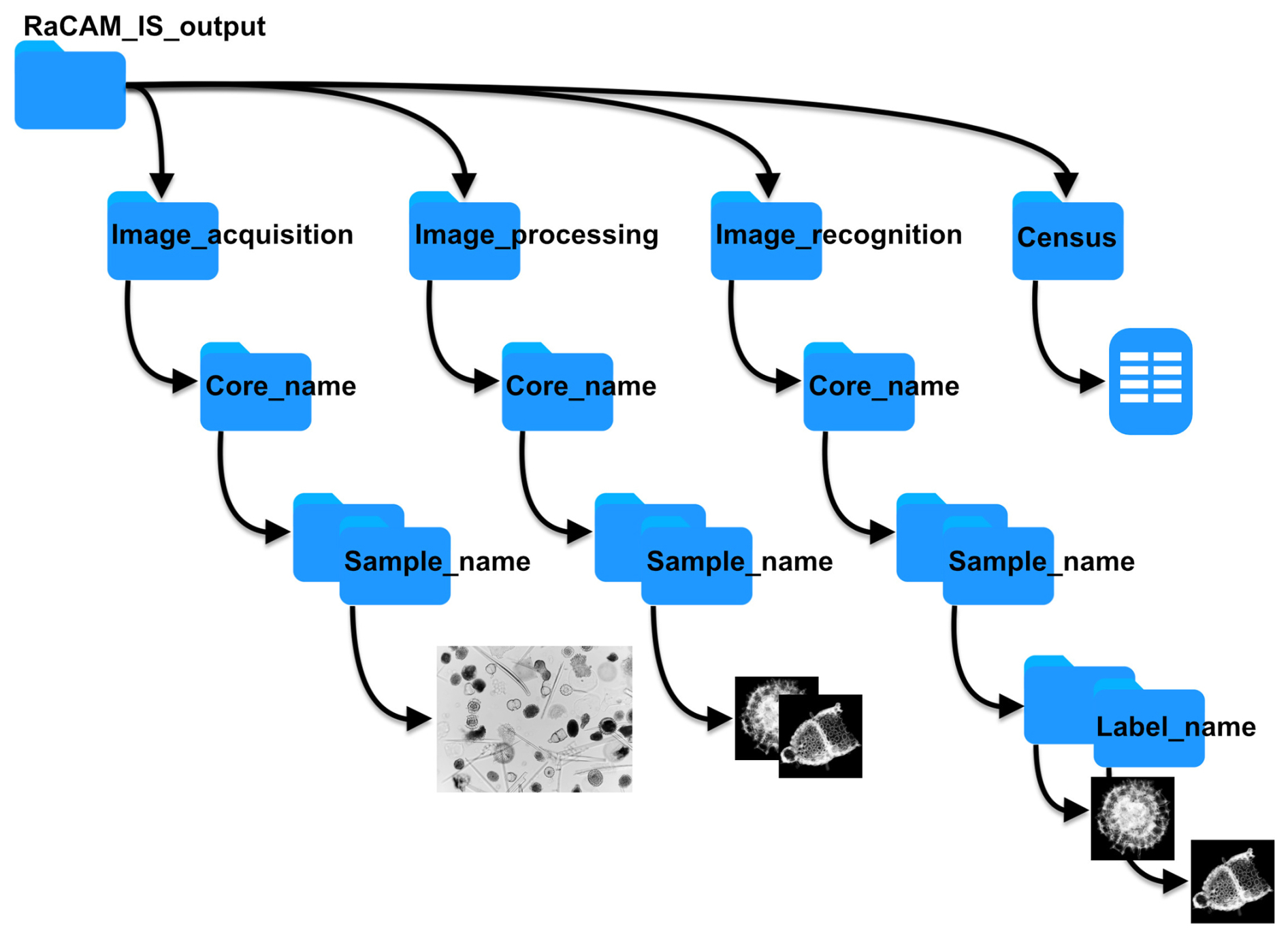
Figure A2 File saving directory structure for the original FOV images, segmented object images, labelled object images, and census data files for the RaCAM_IS software.

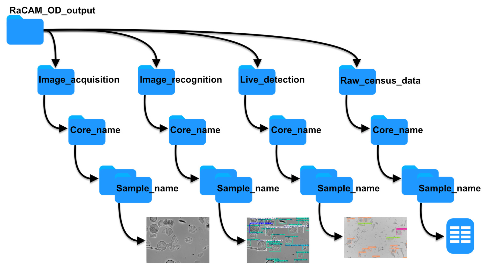
Figure A3 File saving directory structure for the original FOV images, annotated images, live detection images, and census data files for the RaCAM_OD software.