A global spatially contiguous solar-induced fluorescence (CSIF) dataset using neural networks

Satellite-retrieved solar-induced chlorophyll fluorescence (SIF) has shown great potential to monitor the photosynthetic activity of terrestrial ecosystems. However, several issues, including low spatial and temporal resolution of the gridded datasets and high uncertainty of the individual retrievals, limit the applications of SIF. In addition, inconsistency in measurement footprints also hinders the direct comparison between gross primary production (GPP) from eddy covariance (EC) flux towers and satellite-retrieved SIF. In this study, by training a neural network (NN) with surface reflectance from the MODerate-resolution Imaging Spectroradiometer (MODIS) and SIF from Orbiting Carbon Observatory-2 (OCO-2), we generated two global spatially contiguous SIF (CSIF) datasets at moderate spatiotemporal (0.05^∘ 4-day) resolutions during the MODIS era, one for clear-sky conditions (2000–2017) and the other one in all-sky conditions (2000–2016). The clear-sky instantaneous CSIF (CSIF_clear-inst) shows high accuracy against the clear-sky OCO-2 SIF and little bias across biome types. The all-sky daily average CSIF (CSIF_all-daily) dataset exhibits strong spatial, seasonal and interannual dynamics that are consistent with daily SIF from OCO-2 and the Global Ozone Monitoring Experiment-2 (GOME-2). An increasing trend (0.39 %) of annual average CSIF_all-daily is also found, confirming the greening of Earth in most regions. Since the difference between satellite-observed SIF and CSIF is mostly caused by the environmental down-regulation on SIF_yield, the ratio between OCO-2 SIF and CSIF_clear-inst can be an effective indicator of drought stress that is more sensitive than the normalized difference vegetation index and enhanced vegetation index. By comparing CSIF_all-daily with GPP estimates from 40 EC flux towers across the globe, we find a large cross-site variation (c.v. = 0.36) of the GPP–SIF relationship with the highest regression slopes for evergreen needleleaf forest. However, the cross-biome variation is relatively limited (c.v. = 0.15). These two contiguous SIF datasets and the derived GPP–SIF relationship enable a better understanding of the spatial and temporal variations of the GPP across biomes and climate.

1 Introduction

Obtaining a spatiotemporal continuous photosynthetic carbon fixation or gross primary production (GPP) dataset is crucial to food security, ecosystem service and health evaluation, and global carbon cycle studies (Beer et al., 2010). However, this is not possible without remote sensing data, since in situ carbon flux measurements, such as FLUXNET (Baldocchi et al., 2001), are usually costly and have limited spatial and temporal coverage (Schimel et al., 2015). Many remote-sensing-based productivity efficiency models (PEMs) have been built, but the model structure and parameterizations differ from each other and the performance of most models is not satisfactory in terms of simulated interannual variability and trends (Anav et al., 2015; Chen et al., 2017).

Müller (1874) found that the chlorophyll fluorescence (Chl F) from a dilute chlorophyll solution was much stronger than the Chl F from a green leaf, suggesting that an alternative energy pathway exists for leaves in vivo. In the 1980s, scientists found that plant photosynthesis and heat dissipation are two alternatives to quench the excited chlorophyll, and there is a close linkage between Chl F and carbon assimilation rate (Genty et al., 1989; Krause and Weis, 1991). Leaf-level photosynthesis (A_leaf) and fluorescence (Chl F) share the same source of energy originating from photosynthetically active radiation (PAR) absorbed by chlorophyll (APAR_chl), which can be written using a light-use efficiency (LUE) approach (Monteith, 1972):

$$\begin{array}{}\text{(1)}& {\displaystyle }& {\displaystyle }\mathrm{Chl}F=\mathrm{PAR}\times f{\mathrm{PAR}}_{\mathrm{chl}}\times {\mathit{\varphi }}_F\text{(2)}& {\displaystyle }& {\displaystyle }{A}_{\mathrm{leaf}}=\mathrm{PAR}\times f{\mathrm{PAR}}_{\mathrm{chl}}\times {\mathit{\varphi }}_{\mathrm{P}},\end{array}$$

where ϕ_F and ϕ_P represent the efficiencies for Chl F emission and photochemistry, respectively. fPAR_chl, being different from the conventional definition of fraction of photosynthetically active radiation absorption, only considers the fractions absorbed by chlorophyll pigments where the photosynthesis and fluorescence originate (Zhang et al., 2018c). However, Chl F measurements have been mostly conducted at the leaf level, using pulse amplitude modulation (PAM) fluorometers (Porcar-Castell et al., 2008; Roháček and Barták, 1999). In this case, the measured Chl F intensity is not induced by the Sun but by the modulated light source. Although the absolute value of the Chl F intensity does not directly link to A_leaf, it can still be used to calculate the fluorescence yield and investigate the reaction mechanism of the energy partitioning during the light reaction, and to calculate the quantum yield for photochemistry or as a tool to detect plant reactions under stress (Adams and Demmig-Adams, 2004; Flexas et al., 2002).

The successful retrieval of solar-induced (steady-state) chlorophyll fluorescence (SIF) from satellites has made it possible for vegetation photosynthetic activities to be observed at the global scale (Frankenberg et al., 2011; Guanter et al., 2012; Joiner et al., 2011, 2013). Satellite SIF can be expressed as a function similar to the Chl F at the leaf level but with extra terms considering the radiative transfer within the canopy and through the atmosphere (Joiner et al., 2014):

$$\begin{array}{ll}{\displaystyle }& {\displaystyle }{\mathrm{SIF}}_{\mathrm{sat}}\left(\mathit{\lambda }\right)=\mathrm{PAR}\times f{\mathrm{PAR}}_{\mathrm{chl}}\times {\mathrm{\Theta }}_F\left(\mathit{\lambda }\right)\times f_{\mathrm{esc}}(\mathit{\lambda },{\mathit{\theta }}_{\mathrm{s}},{\mathit{\theta }}_{\mathrm{v}},\mathit{\varphi })\\ \text{(3)}& {\displaystyle }& {\displaystyle }\times {\mathit{\tau }}_{\mathrm{atm}}(\mathit{\lambda },{\mathit{\theta }}_{\mathrm{s}},{\mathit{\theta }}_{\mathrm{v}},\mathit{\varphi }),\end{array}$$

where the satellite-retrieved SIF (SIF_sat), fluorescence yield (Θ_F), f_esc and τ_atm are all functions of the wavelength (λ); in addition, f_esc and τ_atm are also affected by sun-sensor geometry characterized by Sun zenith angle (SZA; θ_s), view zenith angle (θ_v) and relative azimuth angle (ϕ). f_esc is a factor describing how much SIF emitted by the chloroplast leaves the canopy, and τ_atm is a function of atmospheric optical depth, which indicates how much SIF that leaves the canopy top passes through the atmosphere before it is captured by the satellite sensors. It should be noted that the fraction of PAR for fluorescence (fPAR_F) may have a different activation spectrum than that for photosynthesis (fPAR_chl), but this difference is ignored here for simplicity. Although additional factors come into play during this process, satellite-retrieved SIF shows high consistency with GPP using both model simulations and ground-based measurements from eddy covariance (EC) flux towers, at least at the monthly timescale (Guanter et al., 2014; Li et al., 2018a; Zhang et al., 2016c, b). In addition, recent studies suggest that the GPP–SIF relationship is consistent across biome types (Sun et al., 2017). This finding, if valid across all biomes, would greatly benefit the usage of SIF for model benchmarking (Luo et al., 2012) and global GPP estimation.

However, several issues hinder exploring the relationship between SIF and in situ GPP estimates. Since the SIF signal is very small and sensors used to retrieve SIF were not initially built to estimate SIF, the satellite-retrieved SIF usually has a large footprint and large uncertainties in individual retrievals (Frankenberg et al., 2014; Joiner et al., 2013, 2016). For instance, the SIF retrieval from the Global Ozone Monitoring Experiment-2 (GOME-2) has a footprint of 40 km×40 km or larger, and the SIF from the Greenhouse gases Observing SATellite (GOSAT) has a circular footprint with 10.5 km in diameter. Direct comparison between the satellite-retrieved SIF signal and GPP estimates from EC flux tower sites thus faces the problem of spatial inconsistency except in areas of large homogenous landscape, e.g., the US Midwest cropland (Zhang et al., 2014) or boreal evergreen forests (Walther et al., 2016). However, corn (C4 pathway) and soybean (C3 pathway) in SIF footprints have different electron use efficiencies (Guan et al., 2016), which should affect the relationship between SIF and GPP. The low precision of SIF measurements also leads to a need for averaging multiple pixels either in space or time before being used.

SIF retrieved from the Orbiting Carbon Observatory-2 (OCO-2) satellite partially solved this issue with a much smaller footprint size (1.3 km×2.25 km), higher signal-to-noise ratio compared to GOSAT (relatively higher SIF retrieval accuracy) and much larger numbers of observations per day (Frankenberg et al., 2014; Sun et al., 2018). However, due to the sparse sampling strategy and long revisit cycle, the OCO-2 SIF data have large gaps between nearby swaths, and the average sampling frequency for each flux tower site is only 3.21 year⁻¹ during 2015–2016 (Lu et al., 2018). In addition, OCO-2 is often aggregated to a monthly dataset at relatively coarse spatial resolution, typically at $\mathrm{1}{}^{\circ }\times \mathrm{1}{}^{\circ }$, which limits its application in small regions. Although several statistical methods have been proposed to downscale satellite observations to finer spatial–temporal resolutions (Tadić et al., 2015, 2017), considering the large land surface heterogeneity and wide gaps between OCO-2 swaths (∼100 km), it could be challenging to apply these methods to OCO-2 SIF.

A high spatiotemporal resolution SIF dataset is needed to improve our understanding of the relationship between SIF and GPP and provide accurate GPP estimates at the global scale. As discussed previously, the satellite-observed SIF contains signals from APAR_chl, fluorescence yield, and canopy and atmospheric attenuation. APAR_chl is considered to be the first-order approximation of SIF as it exhibits high correlation with SIF at the canopy scale (Du et al., 2017; Rossini et al., 2016; Verrelst et al., 2015; Zhang et al., 2018c). Previous studies have shown that fPAR_chl can be inversely estimated using the surface reflectances and radiative transfer models (Zhang et al., 2005, 2016a). The canopy structure information that affects the SIF reabsorption within canopy is also embedded in the near-infrared reflectance (Badgley et al., 2017; Knyazikhin et al., 2013; Yang and van der Tol, 2018). Many previous studies have shown high correlation between SIF and vegetation indices (VIs), especially VIs related to the chlorophyll concentration (Frankenberg et al., 2011; Guanter et al., 2012). Therefore, broadband surface reflectances may have the potential to be used to estimate vegetation information and reconstruct global SIF (Duveiller and Cescatti, 2016; Gentine and Alemohammad, 2018a). However, physical models that can predict SIF (e.g., the Soil Canopy Observation, Photochemistry and Energy fluxes, SCOPE; van der Tol et al., 2009) often require many parameters, making it difficult to use reflectance and modeling to predict SIF at a larger scale.

Neural networks (NNs), together with many other machine learning algorithms, have been used with remote sensing datasets in the Earth sciences, especially for carbon and water fluxes estimation (Alemohammad et al., 2017; Jung et al., 2011; Tramontana et al., 2016), land cover mapping (Kussul et al., 2017; Zhu et al., 2017), soil moisture retrievals and downscaling (Alemohammad et al., 2018; Kolassa et al., 2018) or to bypass parameterization (Gentine et al., 2018). These studies mostly attempted to link the satellite signals with limited in situ observation or model simulations for model training, while taking advantage of the large amount of data in remote sensing observations; they applied the trained algorithm to generate a regional or global dataset. Reconstructing SIF from surface reflectance, on the other hand, uses no in situ observations but faces more problems related to the satellite data quality assurance. The SIF–reflectance relationship is complicated, and the NN benefits from the fact that an explicit physical and radiative transfer relationship is not required.

In this study, we aim to generate a global contiguous SIF (CSIF) product based on the SIF retrievals from OCO-2 and surface reflectances from Moderate-resolution Imaging Spectroradiometer (MODIS) aboard the Terra and Aqua satellites. The CSIF dataset aims to fill the spatial gaps between the OCO-2 swaths and temporal gaps due to the long revisit cycle of OCO-2. Specifically, we first trained and validated the NN using the satellite-observed instantaneous SIF under clear-sky conditions so that the relationship is not affected by cloud-related artifacts. We further generated two SIF products, namely the clear-sky instantaneous SIF (CSIF_clear-inst) and the all-sky daily SIF (CSIF_all-daily). The spatiotemporal variations of these CSIF products were analyzed and compared with SIF from OCO-2 and three other GOME-2 SIF datasets. Finally, we showed two applications of CSIF datasets: (1) monitoring drought impact using CSIF_clear-inst and OCO-2 SIF; (2) evaluating the GPP–SIF relationship by comparing CSIF with GPP estimates from 40 flux tower sites.

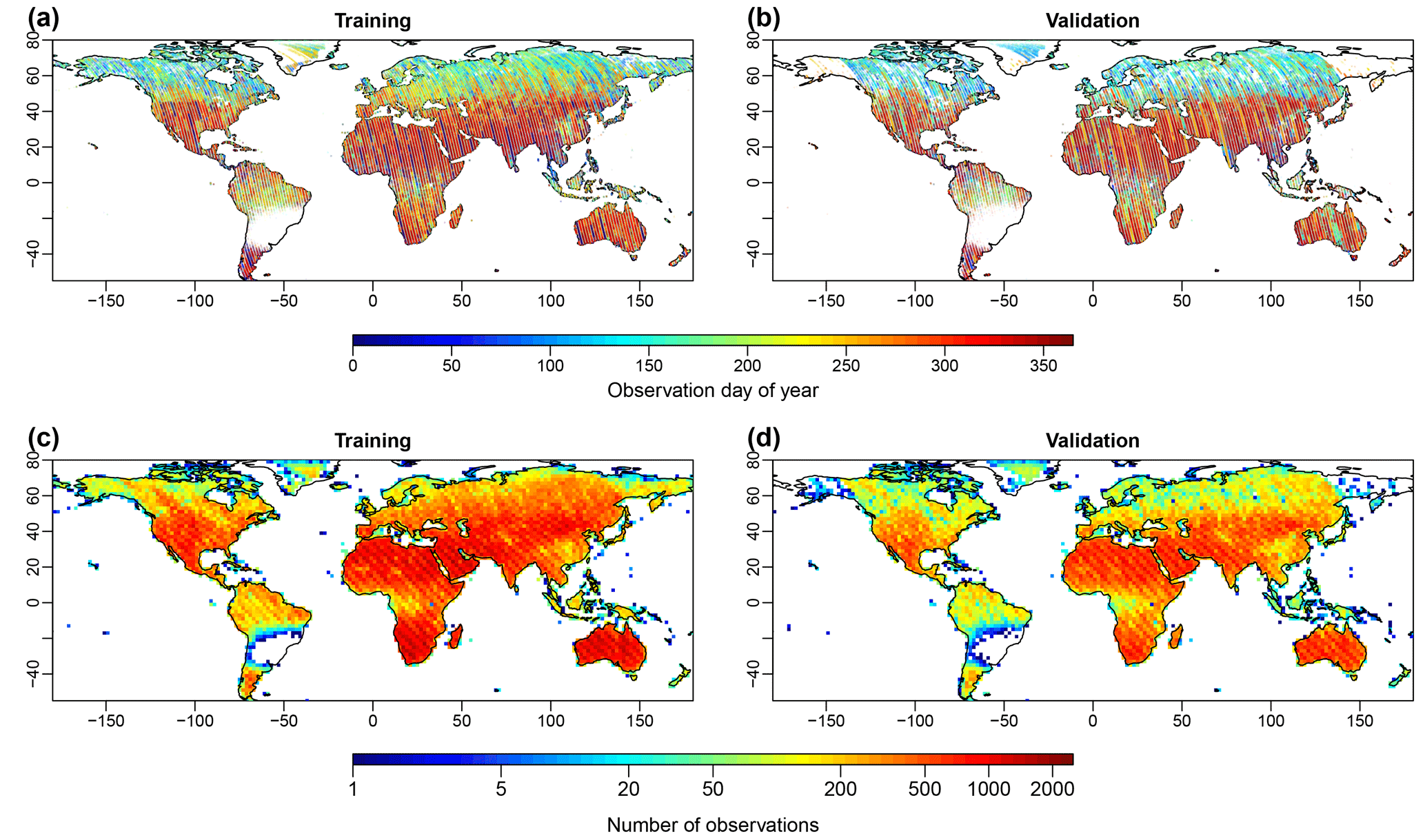
Figure 1 Samples that were used for NN training (years 2015 and 2016) and validation (2014 and 2017). Panels (a) and (b) show the spatial distribution of observation day of year (DOY) and panels (c) and (d) show the spatial distribution of the sample density. Each point in panels (a) and (c) represents a 0.05^∘ training grid cell. Limited observations in South America were caused by the South Atlantic Anomaly (Sun et al., 2018).

2 Materials and methods

2.1 OCO-2 solar-induced chlorophyll fluorescence dataset

The 8100r OCO-2 SIF data between September 2014 and December 2017 were used for NN training and evaluation (Frankenberg, 2015; Frankenberg et al., 2014; Sun et al., 2018). The daily sounding-based SIF retrievals at 757 nm were first aggregated to 0.05^∘ (around 5.6 km×5.6 km at the Equator), consistent with MODIS Climate Modeling Grid (CMG) resolution. The reasons for using this resolution include the following: (1) it is directly comparable (of the same order of magnitude) to the OCO-2 SIF footprint size (around 1.3 km×2.25 km) and the samples within each grid cell can be more evenly distributed and thus more representative of the grid cell SIF values than using much coarser $\mathrm{1}{}^{\circ }\times \mathrm{1}{}^{\circ }$ or $\mathrm{2}{}^{\circ }\times \mathrm{2}{}^{\circ }$ grids; (2) by averaging multiple observations, the uncertainty in the SIF signal can be approximately reduced by a factor of $\sqrt{n}$ (n is the number of observations within this grid cell), assuming independent estimates and homogeneous SIF value within each grid cell (Frankenberg et al., 2014). During this aggregation, we only used cloud-free observations indicated by the OCO-2 cloud flag. For each 0.05^∘ grid cell, the SIF value was only calculated when it contained more than five cloud-free SIF soundings. Although several studies have shown that SIF at different wavelengths has different sensitivity to stress and leaf and canopy reabsorption (Porcar-Castell et al., 2014; Rossini et al., 2015, 2016), we only use SIF at 757 nm since it showed superior performance to SIF at 771 nm in predicting GPP (Li et al., 2018a). The years 2015 and 2016 were used for training and 2014 and 2017 were used for validation. Altogether, 2 947 819 SIF grid cells passed quality check during 2014–2017. Figure 1 shows the spatial distribution of the SIF grid cells used for training and validation (test). It should be noted that the OCO-2 satellite started obtaining data from September 2014 and experienced some malfunctioning during August and September in 2017, causing lower coverage for validation samples in boreal regions.

In addition to these cloud-free observations, we also calculated the all-sky SIF at 0.05^∘ resolution. All SIF retrievals that passed the suggested quality checks (documented in detailed by Sun et al., 2018) were used for the aggregation. The aggregated all-sky instantaneous SIF retrievals were converted to daily values based on the solar zenith angle (Zhang et al., 2018a). We used this dataset to validate the all-sky daily SIF (CSIF_all-daily) (see Sect. 2.5). In both cloud-free and all-sky aggregations, only observations from the nadir mode were used since glint mode tends to underestimate SIF (Sun et al., 2018).

2.2 MODIS reflectance dataset (MCD43C4 V006)

We used the 0.05^∘ daily nadir bidirectional reflectance distribution adjusted reflectance (NBAR) product from MODIS (MCD43C4 V006) during 2000–2017 as input variables for the NN. The NBAR product computed the reflectance at a nadir viewing angle for each pixel at local solar noon. Compared to MOD09 or MYD09 surface reflectance product, it removed the angle effects and therefore should be more stable and consistent (Schaaf et al., 2002). This dataset was processed in two different ways for training and prediction. For the training process, following Gentine and Alemohammad (2018a), we extracted the reflectance from the first four bands of MODIS (centered at 645, 858, 469 and 555 nm, respectively) for the corresponding pixels and days when the cloud-free SIF observations were obtained. It should be noted that although the MCD43C4 is generated for each day and can match the daily SIF observations, the MCD43C4 NBAR uses 16 days worth of inputs and so that the reflectances includes the information on other days than the day of interest. However, we consider this to have limited effects since (1) the vegetation growth/changes are continuous in time, (2) the NBAR product uses 16-day data but also emphasizes the specific day of interest (Schaaf, 2018). These four bands were selected because the visible and near-infrared bands included most of the vegetation information and drives the variation of SIF (Verrelst et al., 2015). We also tested using all seven bands with/without the meteorological variables (temperature and vapor pressure deficit, obtained from the OCO-2 SIF lite files) to train the NN, but the improvements in training and validation were very minor (R² increased by less than 0.01; data not shown), and thus we decided not to use it. Since SIF is very sensitive to the incoming solar radiation, using cloud-free training samples can minimize the uncertainty of using cosine of the solar zenith angle as the proxy of incoming PAR. It should be noted that the training dataset may contain snow-affected samples, but these were not removed to get a more realistic prediction of SIF during winter.

For prediction, we first aggregated the daily reflectance to 4 days. The 4-day temporal resolution is selected to reach a balance among application requirements, information redundancy and dataset sizes. During this process, we used a gap-filling and smoothing algorithm to reconstruct the surface reflectance for the four bands. The detailed description of the gap-filling algorithm can be found in Zhang et al. (2017a). In this study, we slightly modified the algorithm by not applying the best index slope extraction (BISE) algorithm and Savitzky–Golay (SG) filter. The reconstructed 4-day 0.05^∘ reflectance together with other datasets allowed us to predict SIF at 4-day 0.05^∘ resolution during 2000–2017. Since this processing does not involve any extra information and only uses the reflectance observations from the successful model inversion, it should be comparable to the reflectance used for NN training.

2.3 Machine learning algorithms

A feed-forward NN is a number of computational nodes (called neurons) structured in a single or multi-layer architecture. Each neuron is connected with all neurons in the previous layer and next layer. The neuron values are calculated using an activation function with a pre-activated value, i.e., the weighted sum of all neurons in previous layer plus biases. The training of the NN attempts to optimize these weights and biases so that the differences between the output variable in the training data and NN prediction are minimized. In this study, we used Tensorflow (https://www.tensorflow.org, last access: 27 September 2018) and built feed-forward networks with one to three layers and two to nine neurons for each layer. After training models with data from 2015 and 2016, we validated the models using the test dataset from the years 2014 and 2017. We then picked the one with best performance and simplest structure for SIF prediction. The rectified linear unit (ReLU) was used as the activation function since it has shown better performance in our application, and the cost function used is the root mean square error (RMSE). We used 50 epochs with a batch size of 1024. Before training, each variable was normalized by its mean and standardized deviation. Since the NN is not deep and there is no sign of overfitting, we did not use any regularization methods during the training.

2.4 Reconstructing the clear-sky instantaneous SIF and daily SIF

During the NN training process, we only used the SIF and reflectance data in clear-sky conditions, and therefore cos(SZA) was used as a proxy of the incoming photosynthetically active radiation at top of canopy. In the prediction process, we also used the calculated cos(SZA) based on the satellite overpass local solar time and latitude. Since we did not consider the cloud and aerosol attenuation of the PAR, this product was referred to as the “clear-sky instantaneous SIF (CSIF_clear-inst)”.

In addition to the clear-sky instantaneous SIF, we also calculated two daily SIF data by assuming that the incoming solar radiation is the only factor that drives the diurnal cycle (Zhang et al., 2018a). All-sky daily SIF (CSIF_all-daily) can be calculated using the clear-sky top-of-canopy radiation (PAR_clear-inst) and the daily average radiation from the Breathing Earth System Simulator (BESS) (Ryu et al., 2018):

$$\begin{array}{}\text{(4)}& {\displaystyle }{\mathrm{CSIF}}_{\text{all-daily}}={\displaystyle \frac{{\mathrm{CSIF}}_{\text{clear-inst}}}{{\mathrm{PAR}}_{\text{clear-inst}}}}\times {\mathrm{PAR}}_{\mathrm{daily}}^{\mathrm{BESS}},\end{array}$$

where PAR_clear−inst was calculated following previous studies that only considered atmospheric scattering (see Appendix A1). Clear-sky daily SIF (CSIF_clear-daily) assumes no cloud throughout the day and can be calculated by multiplying CSIF_clear-inst with a daily correction factor (γ) (Zhang et al., 2018a):

$$\begin{array}{}\text{(5)}& {\displaystyle }{\mathrm{CSIF}}_{\mathrm{clear}-\mathrm{daily}}={\mathrm{CSIF}}_{\mathrm{clear}-\mathrm{inst}}\times \mathit{\gamma }.\end{array}$$

γ is calculated as the ratio between the cos(SZA) during the satellite overpass and the daily averaged cos(SZA).

2.5 GOME-2 SIF (SIF_GOME-2), reconstructed SIF from GOME-2 (RSIF_GOME-2) and SIF^* datasets

In this study, we also used the GOME-2 SIF (SIF_GOME-2), reconstructed SIF from GOME-2 (RSIF_GOME-2) using machine learning and the SIF^* dataset in comparison with our contiguous SIF from OCO-2. The GOME-2 SIF V27 was retrieved using a principle component analysis algorithm in the wavelength range 734–758 nm (Joiner et al., 2013, 2016). The V27 version, compared to the widely used V26, provides daily correction factor and improved bias correction and calibration (https://avdc.gsfc.nasa.gov/, last access: 27 September 2018). The level-3 monthly 0.5^∘ daily average SIF was used to compare with CSIF_all-daily.

RSIF_GOME-2 (Gentine and Alemohammad, 2018a) uses a similar machine learning technique approach to CSIF but the training is based on the biweekly gridded SIF product from GOME-2 and the 8-day MYD09A1 reflectance dataset. Both clear-sky and cloudy-sky SIF are used for NN training. This dataset has a spatial resolution of 0.05^∘ and 8-day temporal resolution. Both RSIF_GOME-2 and CSIF_all-daily were aggregated to the 0.5^∘ and semi-monthly to facilitate the comparison.

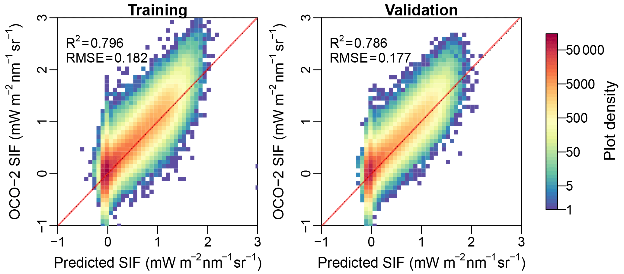
Figure 2 Predicted SIF in comparison with the OCO-2 SIF. Red lines represent the regression slope and the black dotted lines represent the 1:1 line.

The SIF^* dataset (Duveiller and Cescatti, 2016) applies a statistical method and calibrates a model that links monthly 0.5^∘ SIF to the normalized difference vegetation index (NDVI), evapotranspiration (ET) and land surface temperature (LST) dataset for each moving window. The model and its spatiotemporally varied parameters were then applied to finer resolution dataset (NDVI, ET, LST) with a weighted average to generate SIF at 0.05^∘ resolution. In this study, we used the 0.5^∘ monthly SIF^* dataset during 2007–2013 to compare with CSIF.

2.6 Comparing CSIF with GPP at flux tower sites

We further compared the CSIF dataset to GPP estimates from the tier 1 FLUXNET2015 datasets (http://fluxnet.fluxdata.org, last access: 27 September 2018) to investigate the SIF–GPP relationship. Since the CSIF dataset is continuous in space and time, it provides many more samples pairs compared to the original OCO-2 SIF data (Lu et al., 2018). However, because of the landscape heterogeneity and inconsistency between the flux tower footprint and CSIF pixel size, a rigorous site selection is needed. We took the vegetation growth condition into consideration during this process: (1) the annual average, minimum, maximum and seasonal variability (represented by standard deviation) of NDVI (from MOD13Q1 C6) for the target pixel (where the flux tower is located, 250 m by 250 m) need to be similar (within 20 % difference or 0.05 NDVI) to the neighboring (5 km by 5 km) area; (2) the maximum NDVI value for target pixel and neighboring area needs to be greater than 0.2 (not barren). The daily GPP estimates, estimated using nighttime method (Reichstein et al., 2005), were averaged and aggregated into 4-day values to compare with CSIF. The 4-day GPP based on more than 80 % of half-hourly valid (not gap-filled) net ecosystem exchange was retained. Only sites that have at least 92 valid observations (1 year) were used. Only 40 out of 166 sites passed these criteria and were grouped into different biome types (Table S1). In addition to CSIF_all-daily, we also calculated CSIF_clear-daily and CSIF_site which used flux-tower-observed radiation instead of ${\mathrm{PAR}}_{\mathrm{daily}}^{\mathrm{BESS}}$ in Eq. (4).

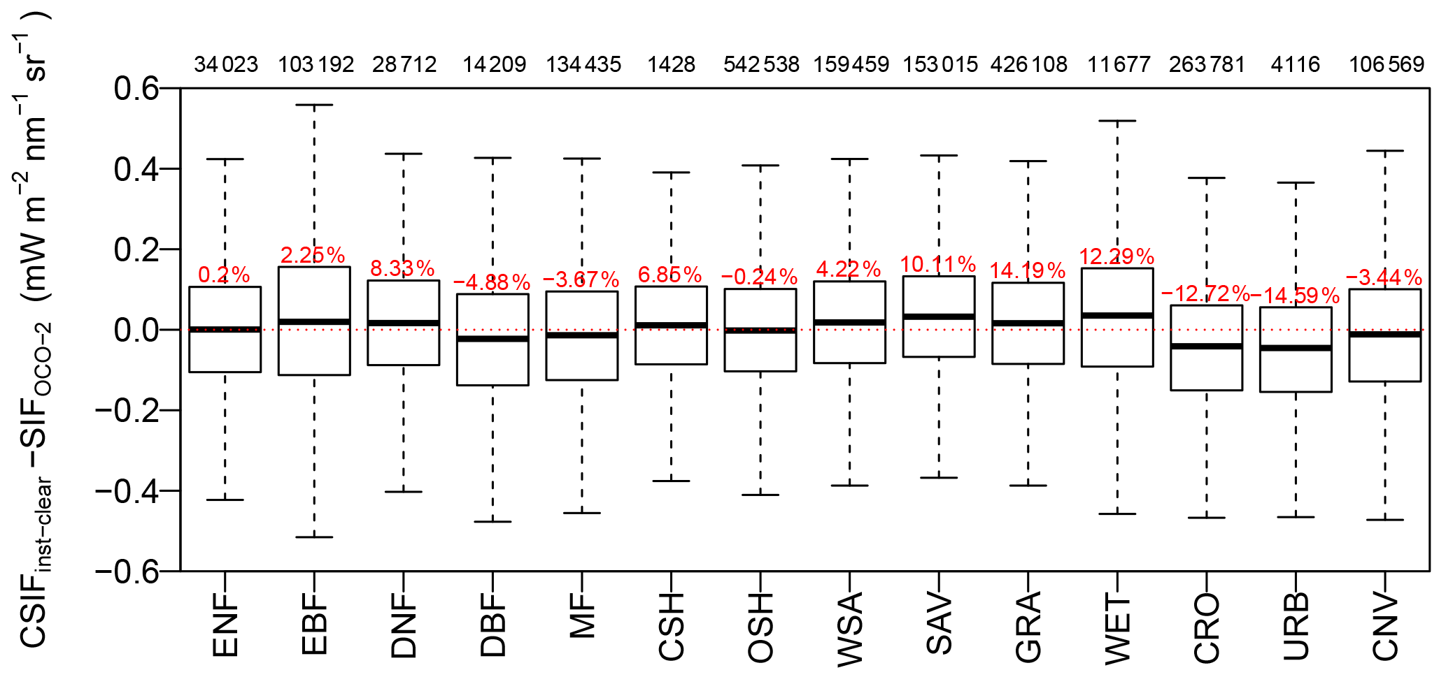
Figure 3 Difference between CSIF_clear-inst and SIF_OCO-2 for major biome types during 2014–2017. The MODIS land cover dataset for 2010 was used to identify the land cover type for each 0.05^∘ grid cell (Friedl et al., 2010). The red percentages above each box represent the mean relative error, and the numbers on top of the figure frame represent the total sample numbers for each biome type. Abbreviations are as follows: ENF, evergreen needleleaf forest; EBF, evergreen broadleaf forest; DNF, deciduous needleleaf forest; DBF, deciduous broadleaf forest; MF, mixed forest; CSH, closed shrubland; OSH, open shrubland; WSA, woody savannas; SAV, savannas; GRA, grassland; WET, wetland; CRO, cropland; URB, urban; CNV, cropland or natural vegetation mosaics.

3 Results

3.1 NN training and validation

The NN with one layer and five neurons generally predicts the OCO-2 SIF during the training with a coefficient of determination (R²) around 0.8 and an RMSE of 0.18 mW m⁻² nm⁻¹ sr⁻¹ (Fig. 2). The model also performs well in the validation (R²=0.79, RMSE = 0.18) and does not show effects of overfitting. Using a variety of layer (one to three) and neuron (two to nine) combinations, we found that one layer with five neurons exhibited slightly higher model performance during the validation compared with a more complex NN (Fig. A1 in Appendix). Therefore, we chose to use the four-band reflectances to feed the one-layer-five-neuron NN to generate the contiguous SIF for 2000 to 2017 when MCD43C4 NBAR dataset is available.

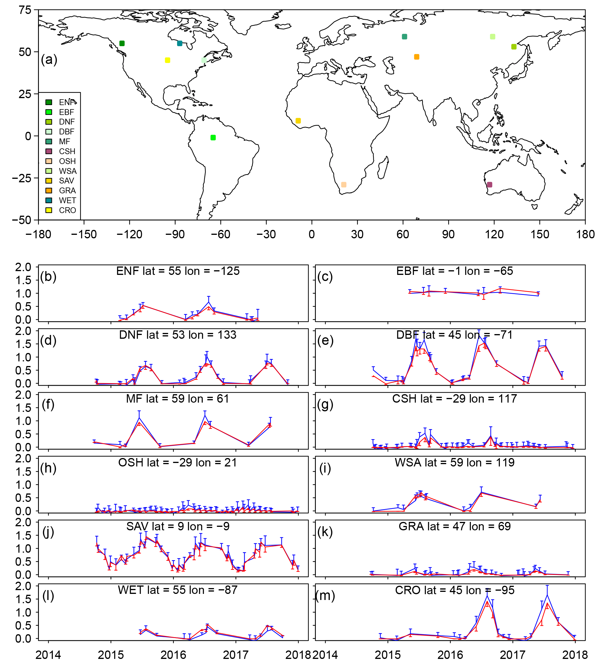
Figure 4 Comparison of predicted SIF by NN and OCO-2-observed SIF for 12 samples ($\mathrm{2}{}^{\circ }\times \mathrm{2}{}^{\circ }$) of major vegetated land cover types during 2014 to 2017. All samples in the training and validation are used. The blue color represents the observed SIF by OCO-2, and the red color represents the SIF prediction by NN. The error bars represent the standard deviation of all $\mathrm{0.05}{}^{\circ }\times \mathrm{0.05}{}^{\circ }$ samples used to generate the $\mathrm{2}{}^{\circ }\times \mathrm{2}{}^{\circ }$ grid boxes. MODIS MOD12C1 V6 land cover dataset is used to select these sample grid boxes.

We also investigated the bias of our prediction among different biome types in Fig. 3. For 9 out of 14 biome types, the differences between the CSIF_clear-inst and the satellite-retrieved SIF are less than 10 %, and most of the biases were within 5 %. Wetlands and urban ecosystem show a 15 % bias compared to the satellite-retrieved SIF, which may be caused by the water or built-up contamination on the reflectance signal and the relatively small sample numbers. For savannas and grassland, the changes in fluorescence yield due to seasonal drought may be important, which cannot be considered in the NN based on reflectances only. Over croplands, CSIF exhibits a 12 % underestimation. The croplands usually have high nitrogen/chlorophyll concentration that may not be fully captured by the four broadband reflectances (Wu et al., 2008). Because we did not build biome-specific NNs for the training, we do not expect biome-specific (especially needleleaf vs. broadleaf) relationships between SIF and reflectance. Interestingly, we still reproduced SIF with very high accuracy regardless of the plant function traits (PFTs), i.e., leaf types and canopy characteristics (leaf clumping, etc.). This suggests that the escape factor and long-term changes in mean fluorescence yield might be correctly accounted for by the NN across PFTs, through the information available in the reflectances only. However, it should be noted that this does not suggest that the NN and reflectances can fully replicate the fluorescence yield variations due to short-term variations caused by stresses.

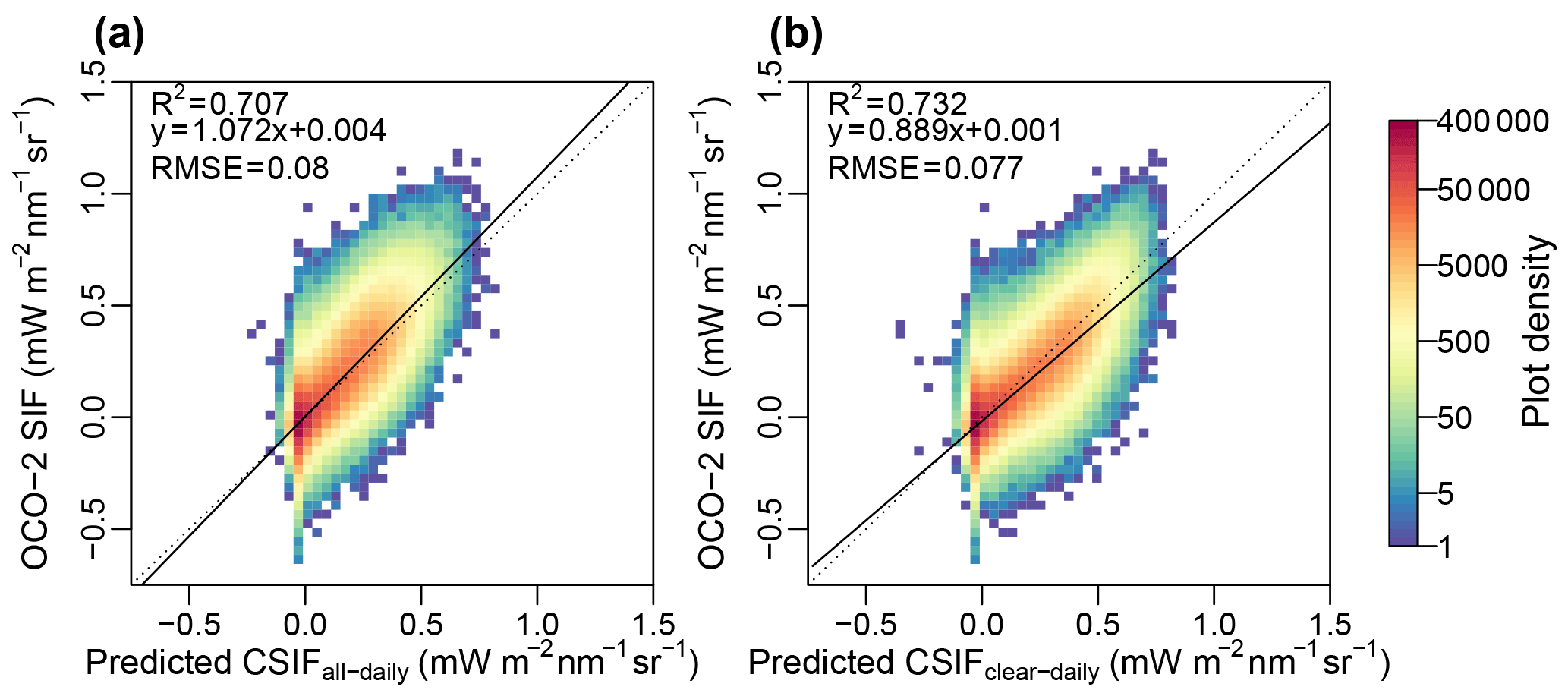
Figure 5 Comparison between the retrieved SIF and the (a) predicted all-sky daily CSIF and (b) clear-sky daily CSIF. The instantaneous SIF retrievals from OCO-2 were converted to daily average values for comparison.

We also compared the time series of predicted CSIF and OCO-2 SIF for 12 typical biome types (Fig. 4). The predicted CSIF accurately captures the seasonal and interannual variation for most biome types, while the standard deviation for each DOY is usually smaller than OCO-2 SIF. This may suggest that the uncertainty of SIF is smaller in CSIF dataset. For some ecosystems, e.g., DBF, MF and CRO, CSIF shows slight underestimation during the peak growing season.

When comparing the daily average SIF from satellite retrievals with the predicted all-sky daily CSIF (CSIF_all-daily) dataset (Fig. 5), the predicted SIF exhibits ∼7 % underestimation, with an R² of 0.71 and a RMSE of 0.08 mW m⁻² nm⁻¹ sr⁻¹. The clear-sky daily CSIF (CSIF_clear-daily) shows ∼11 % overestimation, with a slightly higher R² and lower RMSE. Considering the uncertainty in SIF retrievals and the inconsistency in time of the comparison (satellite SIF was based on instantaneous PAR at the time of satellite overpass and converted to daily values assuming the atmospheric condition did not change within a day; predicted CSIF was based on 4-day average PAR), the all-sky daily CSIF performs reasonably well.

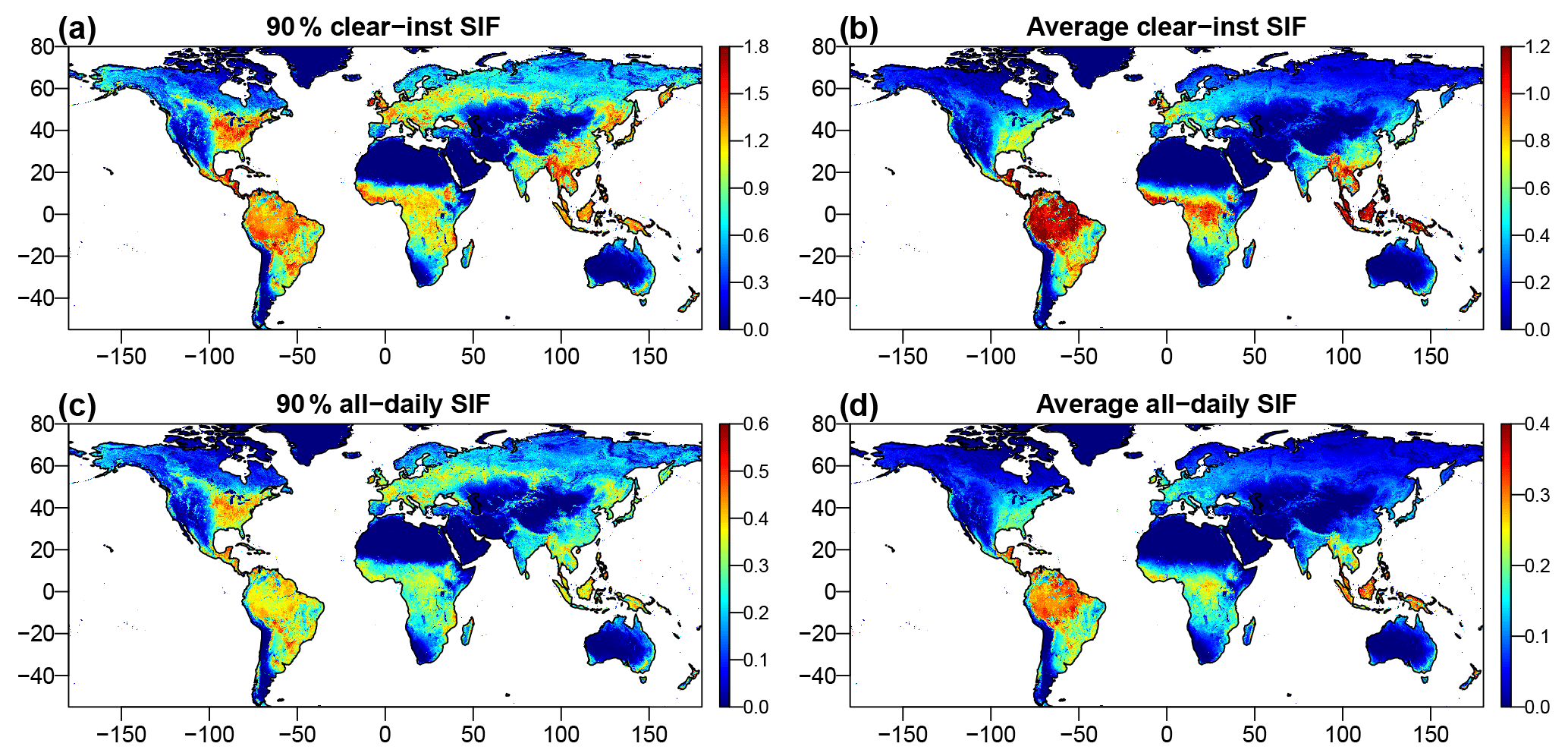
Figure 6 Spatial pattern of maximum (90th percentile) and average daily values for instantaneous clear-sky SIF and all-sky daily SIF. All values are in units of mW m⁻² nm⁻¹ sr⁻¹.

3.2 Spatial–temporal variation of the global 0.05^∘ SIF datasets

Using the trained NN with the gap-filled reflectance datasets, we produced two global CSIF datasets at 4-day temporal and 0.05^∘ spatial resolution. Figure 6 shows the spatial patterns of the 90th percentile for each pixel and the annual average for both clear-sky instantaneous CSIF (CSIF_clear-inst) and the all-sky daily average CSIF (CSIF_all-daily). For the 90th percentile, CSIF_clear-inst exhibits hotspots in the tropical rainforest, south Asia and the North American corn belt, consistent with regions with high peak productivity (Guanter et al., 2014); CSIF_all-daily shows similar spatial patterns but with relatively lower values in the tropical forest, due to the persistent cloud coverage. For the annual average SIF, tropical forests exceed temperate cropland and show very high values for instantaneous clear-sky SIF. In all conditions, African tropical forests exhibit lower values than Amazonian and Southeast Asian tropical forests.

We further investigated the seasonal and interannual variations of the all-sky daily SIF across the latitudes. The tropical regions show continuous high SIF values across seasons, and the northern mid- to high-latitude regions also exhibit recurrent high values during the Northern Hemisphere summers (Fig. 7a). Near 40^∘ S, a hot spot is present in austral summer, with high interannual variability. Low SIF values can be found in dry years (2006–2007, 2009–2010), while high values were observed in wet or normal years (2010–2011, 2012–2015). The global average SIF also displays a strong seasonality coinciding with the Northern Hemisphere growing season (Fig. 7b). For the annual total SIF values, a statistically significant increasing trend (Mann–Kendall test, p<0.0001) is found with around 0.39 % increase per year. The year 2015 exhibited a low anomaly after detrending, which may be caused by the El Niño events (Fig. 7c).

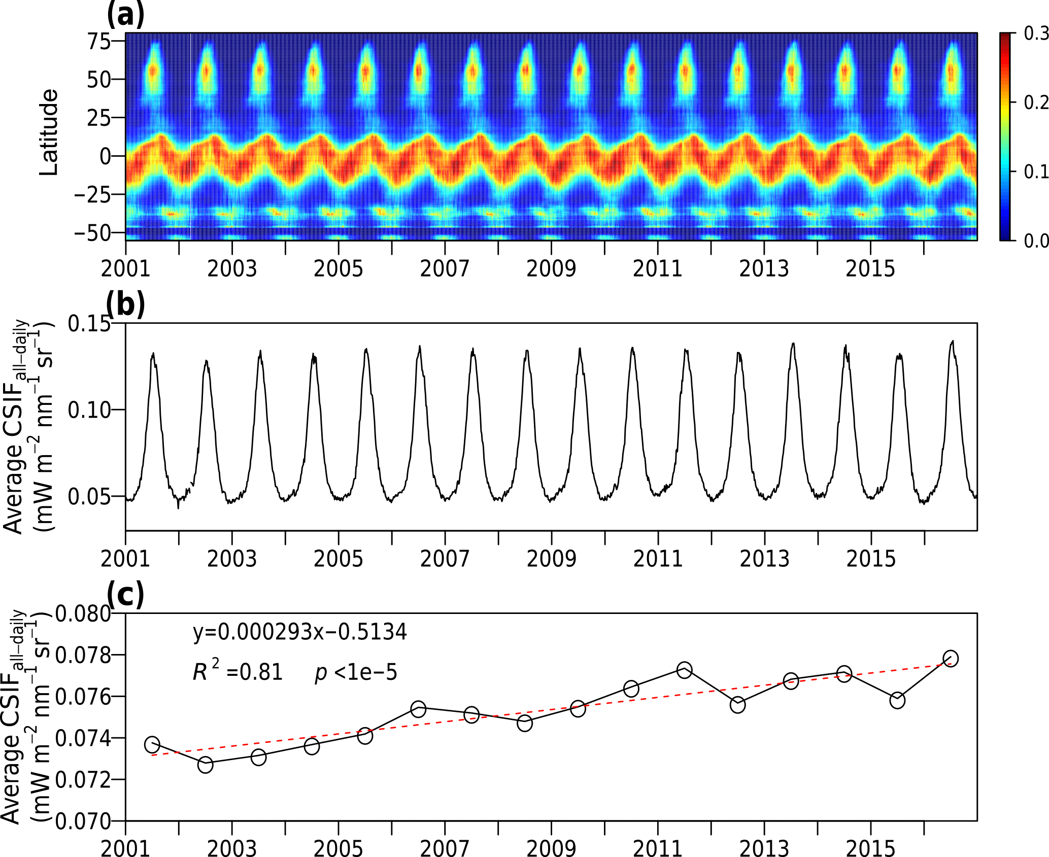
Figure 7 Seasonal and interannual variation of all-sky condition daily CSIF (CSIF_all-daily). (a) The latitudinal averages of CSIF_all-daily for each 4-day period (in mW m⁻² nm⁻¹ sr⁻¹). (b) Global average of CSIF_all-daily for each 4-day period. (c) The annual average CSIF_all-daily between 2001 and 2016 (black line) with linear fit (red dashed line).

Figure 8 Trend of annual average CSIF_all-daily during 2003–2016. The trend is calculated by the Sen's slope estimator. Dots represent the trend is significant (p<0.05) through a Mann–Kendall test. The inset in the bottom left shows the histogram of the CSIF_all-daily trend. Dashed vertical line represents the average trend. Barren areas with an annual average CSIF_all-daily smaller than 0.006 mW m⁻² nm⁻¹ sr⁻¹ are screened from analysis. Trends are in units of mW m⁻² nm⁻¹ sr⁻¹ yr⁻¹.

The spatial pattern of the trend in CSIF_all-daily is displayed in Fig. 8. An increasing trend dominates Europe, southeast Asia and south Amazon. A decreasing trend is mostly found in east Brazil, east Africa and some areas of inland Eurasia. The histogram also shows a positive shift with a magnitude (0.00027 mW nm⁻¹ sr⁻¹ yr⁻¹) similar to the average global trend in Fig. 7c. The spatial pattern of CSIF_all-daily is very similar to the trend pattern of MODIS enhanced vegetation index (EVI) (C6) (Zhang et al., 2017b), but the south Brazilian Amazon forest shows a more positive trend than that of EVI.

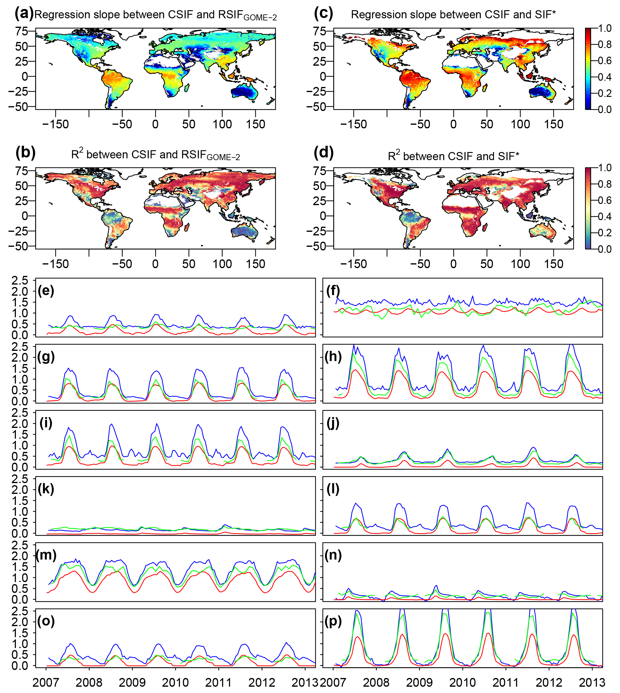
Figure 9 Comparison between CSIF, RSIF_GOME-2 and SIF^* dataset. Regression slopes and coefficient of determination (R²) between the contiguous clear-sky condition instantaneous SIF from OCO-2 (CSIF_inst-clear) and the reconstructed SIF from GOME-2 (RSIF_GOME-2 a, b) or SIF^* (c, d) dataset. The regressions are forced to pass the origin. The CSIF_clear-inst is aggregated to semi-monthly and $\mathrm{0.5}{}^{\circ }\times \mathrm{0.5}{}^{\circ }$ spatial resolution to be consistent with RSIF_GOME-2. Comparison uses the data between 2007 and 2016 (RSIF) or 2007 to 2013 (SIF^*). White regions are barren regions. (e–p) Time series comparison among CSIF (red), RSIF_GOME-2 (blue) and SIF^* (green) for pixels in 12 major land cover types shown in Fig. 4.

3.3 Comparison between SIF from GOME-2 and CSIF

We then compared the CSIF datasets with the reconstructed SIF (RSIF) and SIF^* based on coarser-scale and all-sky GOME-2. Although these datasets were trained based on different satellites, the relationship between CSIF and RSIF or CSIF and SIF^* is consistent across most regions across the globe (Fig. 9). The R² values are generally high (> 0.8) for most regions except over tropical rainforests, barren regions in western US, northwestern China, and northern Canada and Russia. The low R² values are mostly due to the relatively low variability in the temporal domain in the tropics but are also indicative of regions strongly polluted by cloud cover in which CSIF might have a competitive advantage, as the training OCO-2 data better observe the surface due to smaller footprint and with higher signal-to-noise ratio. The regression slopes are higher for regions with persistent cloud cover (e.g., tropical forest). In the time series comparison (Fig. 9e–p), all three SIF datasets show similar seasonal patterns, while GOME-2-based RSIF and SIF^* generally show higher values than CSIF. In addition, RSIF exhibits larger fluctuation during the non-growing season for some sites, which may be caused by snow contamination.

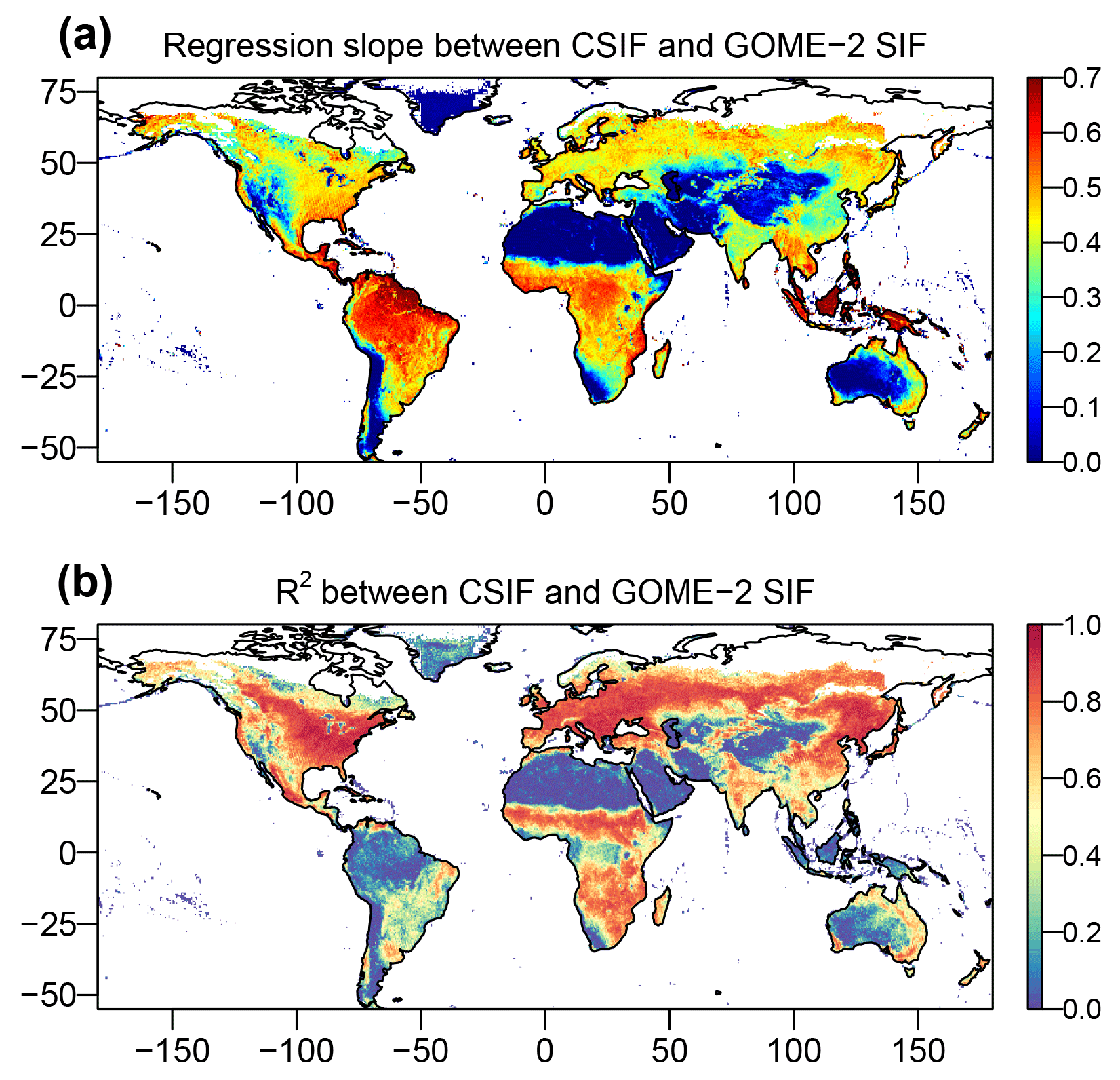
Figure 10 Regression slopes and coefficient of determination (R²) between the contiguous all-sky condition daily SIF from OCO-2 (CSIF_all-daily) and the satellite-retrieved daily SIF from GOME-2 (SIF_GOME-2). The regressions are forced to pass through the origin. The CSIF_all-daily is aggregated to monthly and $\mathrm{0.5}{}^{\circ }\times \mathrm{0.5}{}^{\circ }$ spatial resolution to be consistent with SIF_GOME-2. Comparison uses the data between 2007 and 2016.

We further compared the CSIF_all-daily with GOME-2 daily average SIF (Fig. 10). In general, the correlation is much lower as compared with RSIF for most regions. For regions with high variability in temporal domain, the CSIF_all-daily still shows high R² values with respect to GOME-2 SIF. The regression slopes exhibit smaller variation except for the Amazonian tropical rainforests, southeast Asia and barren regions in the Sahara, western US, northwestern China, central Australia and the Andes mountains in South America. In general, considering the various uncertainties and different satellite overpass times, sensors used and retrieval algorithms, CSIF_all-daily well captured the GOME-2 SIF variations both in space and time. In addition, since GOME-2 SIF in most Argentina is affected by the South Atlantic Anomaly (SAA), the coefficient of determination values are also lower as compared with Fig. 9.

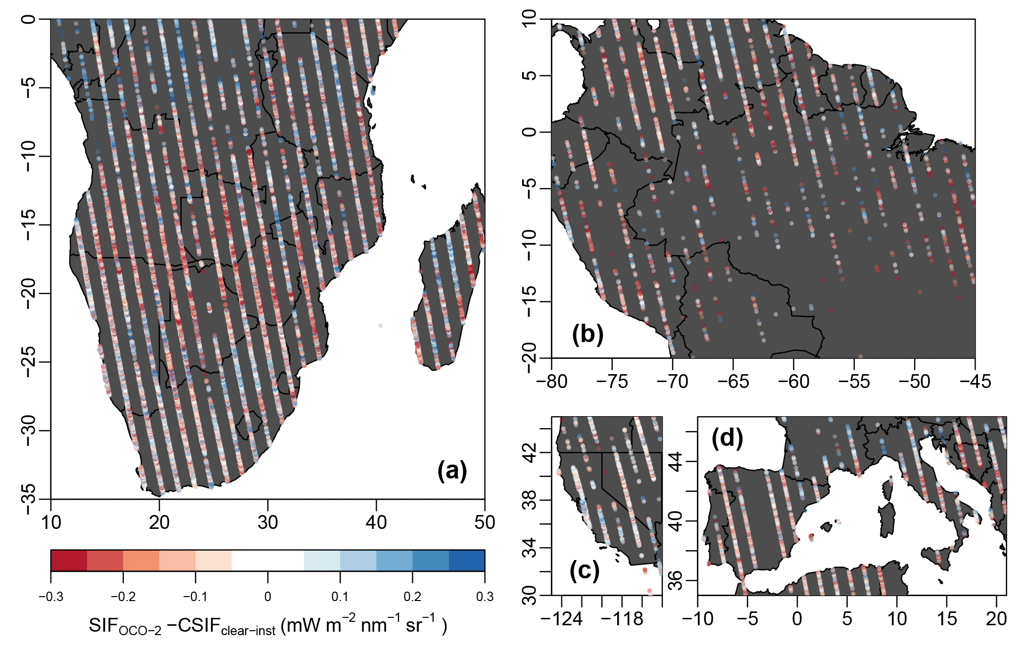
Figure 11 Difference between the OCO-2 SIF and CSIF_clear-inst for four specific drought events during 2014–2017. (a) Southern Africa drought between October 2015 and February 2016. (b) Northeast Amazon drought between January and March 2016. (c) California drought between January and March 2015. (d) Southern Europe drought between July and August 2017.

3.4 Using CSIF for drought monitoring

Since the CSIF dataset only uses broadband reflectances, it should not contain the SIF_yield information. Compared to the SIF retrieved from OCO-2, the difference can be mostly attributed to the SIF_yield. Therefore, the difference or ratio between SIF_OCO-2 and CSIF can reflect the environmental stress on SIF_yield. Figure 11 shows the difference between instantaneous clear-day OCO-2 SIF and CSIF_clear-inst. Except for Fig. 11c, the difference mostly captures the physiological limitation of drought on energy partitioning after being absorbed by chlorophyll. The spatial extent of drought is also well-captured by the difference, where the most severe drought-impacted places also exhibited the largest decline (e.g., Namibia, Botswana, Zimbabwe in Fig. 11a, northeast Amazon in Fig.11b and southern Spain, southernmost France, central Italy, Croatia and Bosnia and Herzegovina). The drought impact on California is less pronounced, possibly because of the irrigation systems and sparse sampling points.

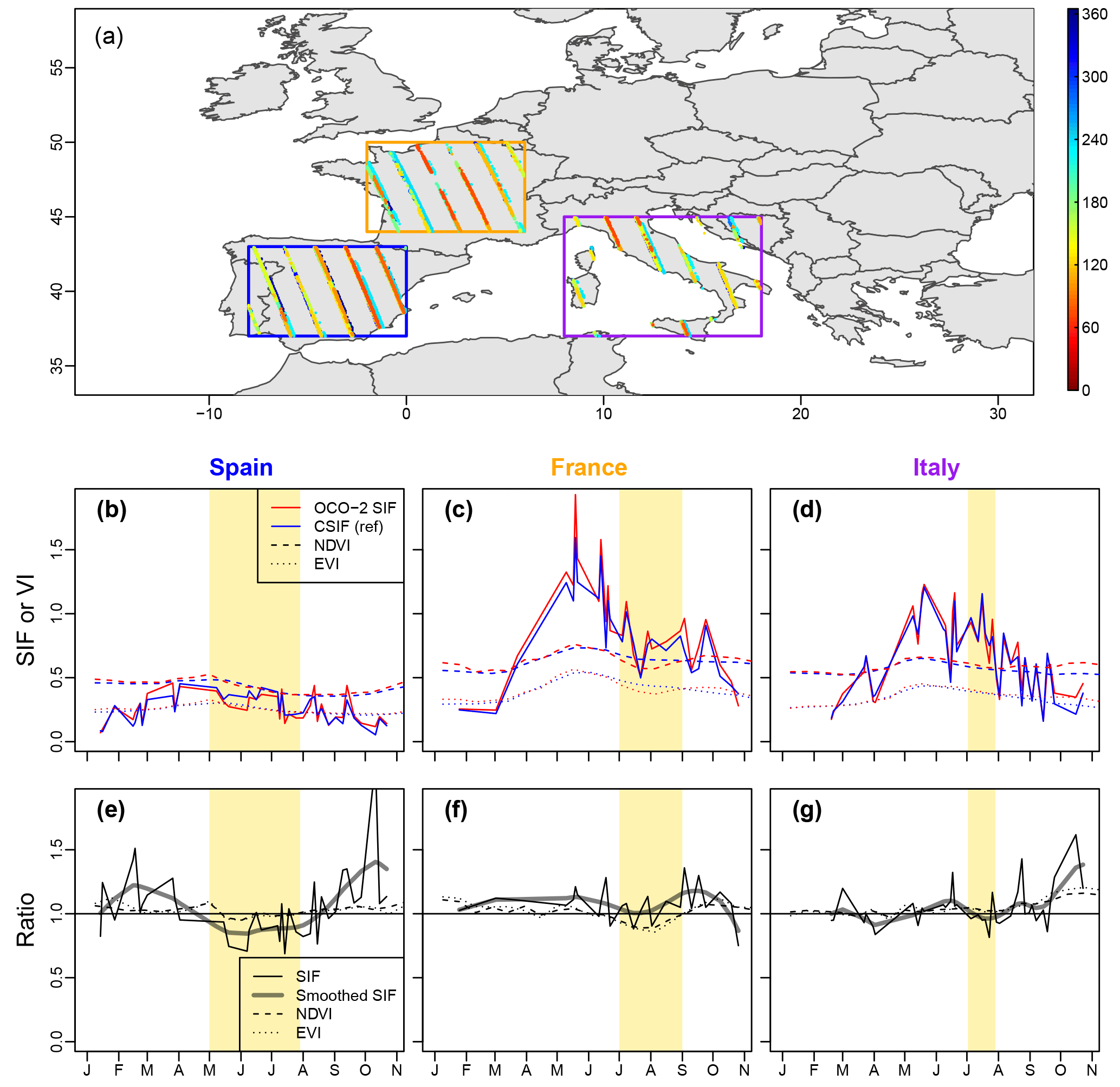
Figure 12 (a) Spatial distribution of OCO-2 SIF observations during 1 January to 1 November in 2015. Different colors represent the observation DOY. (b–d) Average OCO-2 SIF, CSIF NDVI and EVI for the three countries as indicated by three boxes in panel (a). For two vegetation indices, the red color represents the observations in 2015 and blue color represents multi-year average (2000–2014). (e–g) The ratio between OCO-2 SIF and CSIF (SIF) or vegetation indices in 2015 and multi-year average. The thick grey line presents the splines' smoothed SIF ratio.

We further focused on the 2015 European drought to compare the drought response of CSIF and two vegetation indices (NDVI and EVI). Because the OCO-2 samples were not collected at the same swath for each DOY, a large fluctuation can be found in OCO-2 SIF and on the CSIF (which are using the same pixels for a fair comparison) (Fig. 12a–d). However, when calculating the ratio between CSIF and OCO-2 SIF, its variation can be mostly attributed to the variation in SIF_yield, which can quantify the drought stress on plant physiology. In all three regions, the ratio between OCO-2 SIF and CSIF experienced a decrease during the drought period, but the signal is only obvious after applying a smoothing filter. The two vegetation indices, NDVI and EVI, on the other hand, show a reduced response in Spain and Italy, perhaps due to the plants' adaption or very short drought duration.

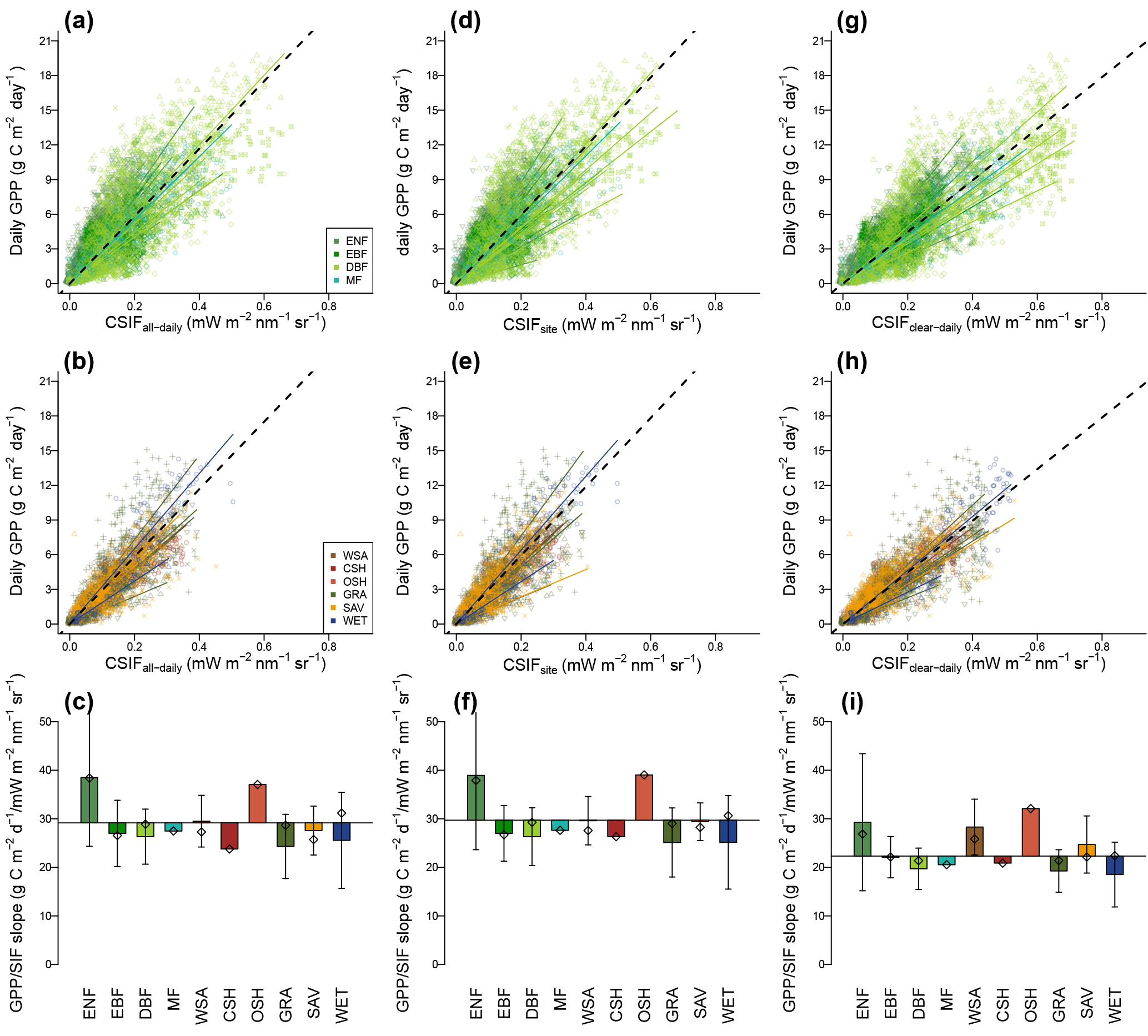
Figure 13 Comparison between GPP estimates from 40 EC flux towers and CSIF_all-daily (a–c) that uses BESS PAR, CSIF_site (d–f) that uses site-measured radiation and CSIF_clear-daily (g–i) that assumes clear-sky condition. The 40 sites were grouped into forests (a, d, g) and non-forests (b, e, h). Color–symbol combinations represent different sites. Summary of the regression slopes between GPP and CSIF for different land cover types (c, f, i). The baseline (dashed black lines) was calculated using all samples (29.71 for CSIF_all-daily, 29.18 for CSIF_site and 22.33 for CSIF_clear-daily). Error bars represent the standard deviation of slopes across sites within this biome type. Rhombuses represent regression for each biome type when data from all sites were combined.

3.5 GPP–CSIF relationship across biome types

With this contiguous SIF_all-daily dataset, we finally evaluated the GPP–CSIF relationship using GPP estimates from 40 flux tower sites from FLUXNET tier 1 dataset. The regression slope between GPP and CSIF (a_GPP∕CSIF) spreads across sites with a regression slope ranging from 11.91 to 68.59 (g C m⁻² day⁻¹/mW m⁻² nm⁻¹ sr⁻¹) for CSIF_all-daily, 11.61 to 72.10 (g C m⁻² day⁻¹/mW m⁻² nm⁻¹ sr⁻¹) for CSIF_site and 11.37 to 62.75 (g C m⁻² day⁻¹/mW m⁻² nm⁻¹ sr⁻¹) for CSIF_clear-daily. The R² value for each individual site ranges from 0.01 to 0.93 with a median value of 0.64, 0.62 and 0.69 for all-daily, site and clear-daily CSIF, respectively. The RMSE is 1.67 g C m⁻² day⁻¹ on average.

Although the CSIF–GPP relationship varies across 40 sites, when lumping all observations within each biome type, the variation is smaller (c.v. = 0.16, rhombus in Fig. 13c, f, i). Specifically, ENF exhibited a significant larger a_GPP∕CSIF (two-tailed Student's t test, p=0.036), which is caused by a stronger canopy reabsorption/scattering of SIF. OSH only has one site and also showed very high value. If both biomes are eliminated, the a_GPP∕CSIF for the other biomes exhibited smaller variation (c.v. = 0.08).

The CSIF–GPP relationship not only varies across biomes but also varies within each biome type, especially for evergreen needleleaf forest (ENF, nine sites), grassland (GRA, eight sites) and wetland (WET, two sites) (Fig. 13c, f). For CSIF_all-daily, the average within-biome variation of a_GPP∕CSIF (c.v. = 0.26±0.08) is comparable to cross-site variations (c.v. = 0.34) but larger than the cross-biome variations (c.v. = 0.16, using the biome-specific CSIF–GPP factor). A similar pattern can be found using CSIF_site or CSIF_clear-daily.

4 Discussion

4.1 Information in contiguous SIF produced by machine learning

Vegetation photosynthetic activity has variations in several respects controlled by vegetation type, phenology, coverage and interactions with the environment. These variations can be expressed in the spatial, seasonal, diurnal and/or interannual domains (Zhang et al., 2018a). Machine learning algorithms try to minimize the differences between the predicted SIF and the satellite-observed SIF. For OCO-2 SIF and the MODIS reflectance used for NN training, the variance in the spatial and seasonal domains is largest. Therefore, the NN generally predicts SIF well in these two domains. The interannual variations (i.e., the variations caused by year-to-year anomalies, e.g., due to drought) typically have much smaller variance and are more difficult to capture. This is why some machine learning products fail to reproduce interannual variability accurately (Jung et al., 2011). Using additional variables that are sensitive to this interannual anomaly in the model training can improve the model performance (Alemohammad et al., 2017; Gentine and Alemohammad, 2018b; Tramontana et al., 2016).

In this study, since the variations in SIF_yield are relatively small (Lee et al., 2015) and cannot be detected by broadband surface reflectances, the SIF_yield information may not be reproduced by our CSIF data. Because the environmental limitation on SIF_yield may be complicated (may not be a linear combination of temperature, vapor pressure deficit (VPD) or surface reflectance in the shortwave infrared) and biome specific (van der Tol et al., 2014), inclusion of other environmental variables and reflectances in shortwave bands during NN training did not greatly increase the SIF prediction accuracy. It should also be noted that SIF_yield is relatively stable when no strong environmental limitation is present (Zhang et al., 2018c). Therefore, the CSIF product should be considered as a good proxy of OCO-2 SIF.

The satellite-retrieved SIF has a relatively large uncertainty for each individual sounding, typically ranging between 0.3 and 0.5 mW m⁻² nm⁻¹ sr⁻¹ (Frankenberg et al., 2014). Previous site-level studies usually use SIF averaged over a large buffered area (Li et al., 2018a; Verma et al., 2017) to reduce the uncertainty. Assuming the uncertainty is unbiased and has a Gaussian distribution, machine learning algorithms are designed to reproduce SIF with lower uncertainty. Compared with previous studies that use light-use efficiency models to downscale SIF to higher resolution (Duveiller and Cescatti, 2016), this study does not rely on multiple modeled input (evapotranspiration, for example) that may introduce additional uncertainties.

We also found a significant increasing trend (0.39 % yr⁻¹) in the global annual CSIF_all-daily (Fig. 7). This trend is close to the GPP trend derived from the satellite-data-driven vegetation photosynthesis model (VPM) (0.32 % yr⁻¹) (Zhang et al., 2017a) but much greater than GPP derived from other remote sensing data-driven models – FLUXCOM (0.01 % yr⁻¹; Tramontana et al., 2016), BESS GPP (0.22 % yr⁻¹; Jiang and Ryu, 2016), MODIS C6 (0.26 % yr⁻¹; Zhao et al., 2005) and WECANN (−0.8 % yr⁻¹, affected by the decreasing GOME-2 SIF trend; Zhang et al., 2018b; Alemohammad et al., 2017). Considering there is no significant trend (−0.02 % yr⁻¹, p>0.1) in BESS PAR (Ryu et al., 2018), this increase is likely caused by the greening of the Earth (Zhang et al., 2017b; Zhu et al., 2016) as captured in the MODIS reflectance data. This increasing trend is also within the range of most Earth system models' predictions (Anav et al., 2015). We also observed a more pronounced increasing trend in the southern Amazon than when using MODIS EVI (Zhang et al., 2017b). This may suggest that CSIF is less likely to suffer from high biomass saturation than optical vegetation indices and can more effectively detect changes in tropical rainforests or over high leaf area regions such as croplands.

4.2 The use of satellite SIF for drought monitoring

Drought can be categorized into different stages. At an early stage, when plants sense water deficit in the soil and higher vapor pressure deficit in the atmosphere, they reduce water loss through stomatal closure. This, in turn, also reduces the CO₂ exchange from stomatal closure and inhibits photosynthesis. The quantum yield for heat dissipation will increase accompanied by a decrease in quantum yield for photochemical quenching and fluorescence (Genty et al., 1989; Porcar-Castell et al., 2014). This should allow satellites to potentially capture this decrease in the SIF signal (especially during the mid-afternoon when stress is more pronounced) as an indicator of vegetation stress. In the second stage, with prolonged dry conditions, plants will recycle the nitrogen in the leaves as represented by a decrease of the greenness (chlorophyll content) of leaves. In the third stage, if the drought continues, leaf senescence and vegetation mortality may follow. SIF can potentially detect changes during all those drought stages, whereas broadband reflectance-based indices (NDVI, EVI) should only see the second and third stages.

Previous drought monitoring studies have mostly used vegetation indices (VIs) as a indictor of drought stress (Ji and Peters, 2003; Zhang et al., 2013). However, vegetation indices can only respond to drought changes in the plants' optical properties (mostly during the second and third stages). For most plants, there might be a tipping point where plants will not recover from drought-induced xylem cavitation (Urli et al., 2013). Since most VIs (e.g., NDVI, EVI) are most sensitive to the canopy changes, drought monitoring based on VIs may not be useful for drought mitigation and agricultural irrigation management. SIF retrievals from satellite, compared to optical reflectance signals, carry the information not only about the PAR absorption by chlorophyll but also about the drought stress on plant physiology. Although previous studies used satellite-based SIF datasets for post-drought impact assessment (Lee et al., 2013; Yoshida et al., 2015; Sun et al., 2015; Wang et al., 2016), these studies did not separate the contribution of decreased APAR_chl or deceased SIF_yield. A more recent study compared the SIF and VIs in India during heat stress (Song et al., 2018) and found that SIF is more sensitive to heat stress than VIs. Similarly, since NDVI and EVI cannot well capture the change in chlorophyll concentration, heat stress on APAR_chl and SIF_yield cannot be fully separated. This study developed a new method to compare the difference between SIF signals and the reflectances, which can be applied for early drought warning at global scale. Although daily OCO-2 data have large gaps between swaths, combining several days of observation can provide enough spatial coverage considering the spatial extent for most drought events. The spatial coverage issues could be further improved using geostatistical-based methods (Tadić et al., 2017), but this may need further investigation. Compared to other meteorological drought indices, this drought monitoring technique uses only near real-time data and avoids the interannual anomalies caused by other factors (land cover change, crop rotation, etc.). The MCD43C4 dataset uses 16 days of inputs for the model inversion, and although this may lead to temporal inconsistencies for the comparison between CSIF and OCO-2 SIF, it may have limited effect due to the higher data quality during drought because of the reduced cloud coverage.

4.3 Cross-biome and within-biome GPP–CSIF relationship

In contrast to Sun et al. (2017), we found a large variation of GPP–CSIF relationship across sites. Compared to previous studies, our study gave higher a_GPP∕CSIF estimates, probably due to a much higher a_GPP∕CSIF value for evergreen needleleaf forest (10 out of 40 sites are ENF) (Table S1 in the Supplement) and slight underestimation of CSIF_all-daily dataset. This higher a_GPP∕CSIF value for ENF was also suggested by the comparison between OCO-2 SIF and FLUXCOM GPP dataset (Sun et al., 2018) and other comparisons using GOSAT SIF (Guanter et al., 2012). Consistent with Li et al. (2018b), we also found small cross-biome variation of the GPP–SIF relationship. However, a large within-biome variation of a_GPP∕CSIF is also found, which contributes to a large proportion of the observed cross-site variations rather than the cross-biome variation. Compared to studies that use OCO-SIF within a large buffering area (e.g., 40 km diameter circle in Verma et al., 2017), we made the comparison over a much smaller area and much higher temporal frequency.

There are several explanations for the observed site-specific GPP–SIF relationship. (1) Leaf morphology may directly affect the reabsorption and scattering of SIF that leaves the foliage (Atherton et al., 2017); however, this factor is not considered in current SIF modeling (van der Tol et al., 2009; Verrelst et al., 2015) and will directly affect the model simulation of the GPP–SIF relationship at the ecosystem scale (Verrelst et al., 2016; Zhang et al., 2016c). (2) Vegetation canopy characteristics also affect the reabsorption and scattering of SIF before leaving the canopy (Romero et al., 2018; Yang and van der Tol, 2018). (3) Atmospheric condition may attenuate and bias satellite SIF retrievals to some extent, but this effect is assumed to be small unless thick clouds are present (Frankenberg and Berry, 2017). (4) SIF and GPP likely have different sensitivities to environmental stresses (Flexas et al., 2002); therefore, ecosystems with frequent environmental stresses (e.g., drought) during the growing season tend to have relatively lower GPP-to-SIF ratio. (5) Since light saturations have less effect on SIF than GPP (Damm et al., 2015; Zhang et al., 2016c), the growing-season averaged light intensity (affected by latitude, average cloud coverage), vegetation canopy structure and leaf characteristics that relate to the light saturation will also affect GPP–SIF relationship. For example, the evergreen needleleaf forests have much higher specific leaf area and usually lower Sun zenith angle, making them less prone to light saturation. These factors may vary not only across biomes but also across sites. Therefore, within one biome type, the GPP–SIF relationship can also be different.

It is also noteworthy that clear-sky daily SIF exhibited stronger correlation with GPP (Fig. 13); a possible explanation would be that the light-use efficiency increases with diffused radiation, which partly compensates for the decrease in incoming PAR when clouds are present (Gu et al., 2002; Turner et al., 2006). Because the satellite SIF retrieval algorithm discarded observations that were affected by thick clouds (Sun et al., 2018), the SIF retrievals from OCO-2 are more positively biased than the actual SIF emission of the plants. However, during periods when thick clouds are present, the LUE also increases and so does the GPP ∕ SIF ratio. The positive SIF retrieval biases compensated the increase in the GPP ∕ SIF ratio and therefore contributed to a stronger correlation between satellite-retrieved SIF (rather than the actual SIF emission) and GPP.

4.4 Uncertainties and caveats

Although our CSIF_clear-inst showed good performance as supported by the comparison with the clear-sky instantaneous SIF retrievals from OCO-2, the CSIF_all-daily exhibits a slight underestimation. A possible explanation is that most SIF retrievals during overcast conditions did not pass the quality checks, such that OCO-2 SIF are more likely obtained during clear-sky conditions. This is supported by the fact that if we compare OCO-2 SIF with clear-daily SIF, the R² is even higher (Fig. 6).

The canopy structure and sun-sensor geometry were not explicitly considered in our modeling and only implicitly embedded in the machine learning retrieval. Several recent studies suggest that canopy structure will affect the PAR absorption and re-absorption of SIF before leaving the canopy (f_esc in Eq. 3) (Knyazikhin et al., 2013; Liu et al., 2016; Yang and van der Tol, 2018) and further affect the GPP–SIF relationship (He et al., 2017; Migliavacca et al., 2017; Zhang et al., 2016c). However, most of these studies made assumptions requiring either a dense canopy or non-reflecting soil and thus cannot be easily applied at the global scale. In addition, OCO-2 SIF data used in this study are from nadir observations, while both the MODIS and GOME-2 sensors acquire images both at nadir and near nadir. Such discrepancy in observation angles may induce bidirectional effects. Since CSIF is trained based on the satellite-observed SIF instead of the canopy SIF emission, and as previously discussed, it did not consider the atmospheric attenuation of SIF signal in the presence of clouds. The CSIF values are expected to be closer to the canopy SIF emission than the satellite-observed SIF at the top of atmosphere.

The BESS PAR 4-day dataset has high overall accuracy (RRMSE of 15.2 %) and very little bias (1.4 %). For different climate zones, the uncertainties are typically under 20 %. These uncertainties do not affect the CSIF_clear-inst data but will propagate to CSIF_all-daily.

5 Conclusions

In this study, using the surface reflectance from the MODIS instrument and a NN algorithm, we developed two spatially contiguous and high-temporal-resolution SIF datasets (CSIF). These two SIF products not only show high accuracy when validated against the satellite-retrieved OCO-2 SIF but also exhibit reasonably high consistency with both reconstructed and satellite-retrieved GOME-2 SIF. CSIF_all-daily exhibits an increasing trend globally during 2001–2016, which is attributed to the Earth greening and not to changes in PAR. Since the CSIF dataset includes most information on PAR absorption of chlorophyll, the difference between OCO-2 SIF and CSIF mostly contains the information on physiological stress on fluorescence yield. This indicator is found to be more effective for early drought warning than vegetation indices. By comparing CSIF_all-daily with GPP estimates across 40 EC flux tower sites, the GPP–SIF relationship is found to vary across sites, and a large proportion of this comes from within-biome variation. However, this finding still requires further examination using SIF from both new satellites instruments (e.g., TROPOMI) and ground-based measurements. The high-resolution CSIF dataset can be further used for regional to global carbon and water flux analysis.

Appendix A: Calculation of clear-sky radiation

We calculated the clear-sky radiation following previous studies (Duffie and Beckman, 2013; Ryu et al., 2018). The total surface shortwave radiation R_T is the summation of direct surface beam radiation (R_sb) and diffused radiation (R_sd):

$$\begin{array}{}\text{(A1)}& R_{\mathrm{T}}=R_{\mathrm{sb}}+R_{\mathrm{sd}}.\end{array}$$

R_sb and R_sd are calculated as the product of the top-of-atmosphere shortwave radiation (R_TOA) and the atmospheric transmittance for beam radiation (τ_b) and that for diffused radiation (τ_d):

$$\begin{array}{}\text{(A2)}& {\displaystyle }& {\displaystyle }{R}_{\mathrm{sb}}=R_{\mathrm{TOA}}\times {\mathit{\tau }}_{\mathrm{b}}\text{(A3)}& {\displaystyle }& {\displaystyle }{R}_{\mathrm{sd}}=R_{\mathrm{TOA}}\times {\mathit{\tau }}_{\mathrm{d}},\end{array}$$

where R_TOA is calculate as a function of solar constant (S₀=1360.8 W m⁻²), the proportion of solar irradiance within shortwave range (α=0.98), the day of year (n) and the cosine of the solar zenith angle (cosθ_s):

$$\begin{array}{}\text{(A4)}& {\displaystyle }{R}_{\mathrm{TOA}}=S_{\mathrm{0}}\times \mathit{\alpha }\times \left[\mathrm{1}+\mathrm{0.033}\cos \left({\displaystyle \frac{\mathrm{2}\mathit{\pi }n}{\mathrm{365}}}\right)\right]\times \cos {\mathit{\theta }}_{\mathrm{s}},\end{array}$$

and τ_b is calculated as

$$\begin{array}{}\text{(A5)}& {\displaystyle }{\mathit{\tau }}_{\mathrm{b}}=a_{\mathrm{0}}+a_{\mathrm{1}}\exp \left({\displaystyle \frac{-k}{\cos {\mathit{\theta }}_{\mathrm{s}}}}\right),\end{array}$$

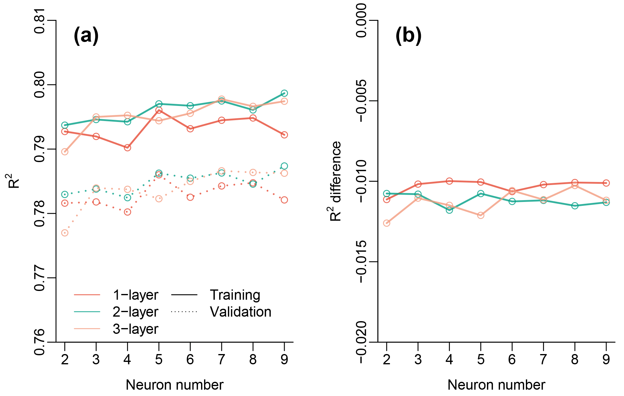
Figure A1 (a) Comparison of model performance (R²) during training and validation with a variety of NN layers (one to three) and neuron numbers for each layer (two to nine). (b) Difference of model performance between the training and validation for different layer and neuron combinations.

where a₀, a₁ and k are coefficients that consider the atmospheric attenuation based on the atmosphere path length and abundance of the gases or particles that need to be adjusted for elevation:

$$\begin{array}{}\text{(A6a)}& {\displaystyle }& {\displaystyle }{a}_{\mathrm{0}}=\mathrm{0.4237}-\mathrm{0.00821}{\left(\mathrm{6}-A\right)}^{\mathrm{2}}\text{(A6b)}& {\displaystyle }& {\displaystyle }{a}_{\mathrm{1}}=\mathrm{0.5055}+\mathrm{0.00595}{\left(\mathrm{6.5}-A\right)}^{\mathrm{2}}\text{(A6c)}& {\displaystyle }& {\displaystyle }k=\mathrm{0.2711}+\mathrm{0.01858}(\mathrm{2.5}-A{)}^{\mathrm{2}},\end{array}$$

where A is the elevation in kilometers. The ETOPO1 Global Relief Model was used to provide the elevation information. This dataset was downloaded from National Oceanic and Atmospheric Administration (https://data.nodc.noaa.gov/, last access: 27 September 2018) and aggregated to 0.05^∘. In this study, we did not consider the variation of these parameters for different climate and latitudinal zones since those effects are less important. The transmittance for diffused radiation (τ_d) is calculated as a function of τ_b:

$$\begin{array}{}\text{(A7)}& {\mathit{\tau }}_d=\mathrm{0.271}-\mathrm{0.294}{\mathit{\tau }}_{\mathrm{b}}.\end{array}$$