the Creative Commons Attribution 4.0 License.
the Creative Commons Attribution 4.0 License.
 | 26 Oct 2018
Assessing the dynamics of vegetation productivity in circumpolar regions with different satellite indicators of greenness and photosynthesis
Sophia Walther
Luis Guanter
Birgit Heim
Martin Jung
Gregory Duveiller
Aleksandra Wolanin
Torsten Sachs
High-latitude treeless ecosystems represent spatially highly heterogeneous landscapes with small net carbon fluxes and a short growing season. Reliable observations and process understanding are critical for projections of the carbon balance of the climate-sensitive tundra. Space-borne remote sensing is the only tool to obtain spatially continuous and temporally resolved information on vegetation greenness and activity in remote circumpolar areas. However, confounding effects from persistent clouds, low sun elevation angles, numerous lakes, widespread surface inundation, and the sparseness of the vegetation render it highly challenging. Here, we conduct an extensive analysis of the timing of peak vegetation productivity as shown by satellite observations of complementary indicators of plant greenness and photosynthesis. We choose to focus on productivity during the peak of the growing season, as it importantly affects the total annual carbon uptake. The suite of indicators are as follows: (1) MODIS-based vegetation indices (VIs) as proxies for the fraction of incident photosynthetically active radiation (PAR) that is absorbed (fPAR), (2) VIs combined with estimates of PAR as a proxy of the total absorbed radiation (APAR), (3) sun-induced chlorophyll fluorescence (SIF) serving as a proxy for photosynthesis, (4) vegetation optical depth (VOD), indicative of total water content and (5) empirically upscaled modelled gross primary productivity (GPP). Averaged over the pan-Arctic we find a clear order of the annual peak as APAR ≦ . SIF as an indicator of photosynthesis is maximised around the time of highest annual temperatures. The modelled GPP peaks at a similar time to APAR. The time lag of the annual peak between APAR and instantaneous SIF fluxes indicates that the SIF data do contain information on light-use efficiency of tundra vegetation, but further detailed studies are necessary to verify this. Delayed peak greenness compared to peak photosynthesis is consistently found across years and land-cover classes. A particularly late peak of the normalised difference vegetation index (NDVI) in regions with very small seasonality in greenness and a high amount of lakes probably originates from artefacts. Given the very short growing season in circumpolar areas, the average time difference in maximum annual photosynthetic activity and greenness or growth of 3 to 25 days (depending on the data sets chosen) is important and needs to be considered when using satellite observations as drivers in vegetation models.
- Article
(17505 KB) - Full-text XML
- BibTeX
- EndNote


Landscapes in circumpolar regions are characterised by sparse vegetation, bare soil, rocks, large surface areas inundated by open water and a long snow-covered period. Despite large carbon amounts being stored in the often permanently frozen grounds, net fluxes of carbon between the land surface and the atmosphere are small and their CO2 balance is close to neutrality (McGuire et al., 2012). Because of their strong sensitivity to environmental conditions, carbon exchange processes are highly variable in space and time (Lafleur and Humphreys, 2008; Olivas et al., 2011; Pirk et al., 2017; Welker et al., 2004) and an ecosystem might switch between being a carbon sink or source from year to year depending on the weather conditions (Huemmrich et al., 2010b).
Warming happens at accelerated rates compared to middle and lower latitudes (AMAP, 2012). The carbon budgets of both the tundra ecosystem and the Arctic boreal zone as a whole are undergoing major changes – with possibly strong feedbacks to climate (Pearson et al., 2013). The future evolution of the net ecosystem exchange (NEE), its component fluxes gross primary productivity (GPP) and respiration in Arctic landscapes is highly uncertain. Higher temperatures, the accompanying mineralization, and higher atmospheric CO2 concentrations fertilise vegetation (Welker et al., 2004; Yi et al., 2014; Zhu et al., 2016). Accordingly, changes in species composition (Chapin et al., 1995) are observed and satellite records indicate a greening in large regions in the Arctic (Jia et al., 2003; Verbyla, 2008). This is interpreted as increased growth (Chapin et al., 1995; Elmendorf et al., 2012; Huemmrich et al., 2010a; Stow et al., 2004) or even as a woody encroachment into tundra (Dass et al., 2016; Stow et al., 2004; Sturm et al., 2001). Yet, higher leaf mass and growth do not necessarily linearly translate into enhanced GPP in every case, as increased growth might also cause enhanced self-shading and lower nitrogen amounts per unit leaf area (McFadden et al., 2003; Street et al., 2007). A warmer climate might extend the snow-free period (Myneni et al., 1997), but there are contradicting indications of whether (Kross et al., 2014; Lund et al., 2010; Ueyama et al., 2013b) or not (Gamon et al., 2013; Lafleur and Humphreys, 2008; López-Blanco et al., 2017; Oberbauer et al., 1998) a longer growing season enhances seasonal carbon uptake and growth. Photosynthetic activity and plant growth further depend on soil moisture conditions (Gamon et al., 2013; Lafleur and Humphreys, 2008; Opała-Owczarek et al., 2018; Welker et al., 2004), therefore warming and shorter and shallower snow packs do not necessarily increase productivity (Gamon et al., 2013; Huemmrich et al., 2010a, b; Parida and Buermann, 2014; Yi et al., 2014; Zhang et al., 2008). Soil warming promotes thaw and stronger drainage. Heterogeneous respiration and carbon emissions into the atmosphere are stimulated in warmer soils at a lowered water table depth (Billings et al., 1982; Commane et al., 2017; Huemmrich et al., 2010b; Oechel et al., 1993; Yi et al., 2014). The balance between the photosynthetic carbon uptake and respirational losses is further modulated by permafrost disturbances (Cassidy et al., 2016). Polar treeless regions are spatially highly heterogeneous ecosystems (Welker et al., 2004) but have widespread full vegetation cover. NEE, GPP and respiration are governed by variable conditions regarding the wetness and temperature, microtopography, geomorphology and type, and acidity of the soils (Emmerton et al., 2016; Kwon et al., 2006; Olivas et al., 2011; Pirk et al., 2017; Walker et al., 1998). It is not clear whether, where and when the land surface in Arctic tundra actually acts as a sink or source of CO2 (Cahoon et al., 2012; McGuire et al., 2012) and what the direction and magnitude of changes in altered climatic conditions will be (Billings, 1987; Oechel et al., 1993; Sitch et al., 2007). This has given rise to extensive and long-term project studies of the Arctic like the Arctic-Boreal Vulnerability Experiment (ABoVE, https://above.nasa.gov/about.html, last access: 22 August 2018) or the Carbon in Arctic Reservoirs Vulnerability Experiment (CARVE, https://carve.jpl.nasa.gov/Missionoverview/, last access: 22 August 2018), both of which are not limited to CO2.
Observing carbon fluxes in these inaccessible and remote areas is difficult. Several long-term monitoring sites exist where phenological observations, spectral reflectance as well as gas flux measurements are conducted in situ, both under natural conditions and in manipulative experiments. Many studies can be found in the literature that evaluate eddy covariance (EC) or the chamber gas flux measurements with respect to the spatial patterns of NEE at a fixed point in time or in situ NEE integrated over the growing season and its variations between years (Kross et al., 2014; Lund et al., 2010; López-Blanco et al., 2017; Marushchak et al., 2013; McFadden et al., 2003; Ueyama et al., 2013a; Williams and Rastetter, 1999). However, only a few sites exist compared to temperate regions, and observations are usually not done in a continuous manner over the complete year but during individual measurement campaigns or dedicated periods during the growing season. Even if automated instrumentation can provide more continuous measurements throughout the year, it is still hampered by the difficulty of access in the case of equipment failure. Compared to more temperate sites, tundra poses additional challenges on the calculation of NEE and its component flux GPP and respiration (Pirk et al., 2017). Due to the small magnitudes of the net fluxes, different flux calculation methods might even differ in whether they indicate a source or a sink at a given time (Pirk et al., 2017). Snow and soil freezing can act as a barrier for gas exchange with the atmosphere and cause a temporal decoupling between the registration at the sensors and when the gas concentrations have actually been changed by the heterotrophic respiration in the soil (Arneth et al., 2006) or by the photosynthesis of evergreens under the snow (Starr and Oberbauer, 2003). Continuous illumination during the polar day challenges temperature–respiration relationships obtained from night-time data (Runkle et al., 2013). Further, the heterogeneity of the landscape poses limits to the spatial representativeness of the relationships between the carbon fluxes and meteorological and soil conditions that have been identified in situ (Pirk et al., 2017; Tuovinen et al., 2018). Therefore, in spatial up-scaling exercises (Huemmrich et al., 2013; Marushchak et al., 2013; Tramontana et al., 2016; Ueyama et al., 2013a), strong extrapolations are necessary. Yet, the modelling of the future evolution of the vegetation and carbon fluxes (including their timing and magnitude) in circumpolar areas requires an understanding of GPP and respiration as well as accurate spatially and temporally explicit observations of their drivers.
Satellite remote sensing can help in constraining the component flux of GPP and additionally in extending point observations to larger areas with repetitive coverage in time. Depending on the monitoring approach, different assets and limitations need to be considered to infer GPP. Optical reflectance measurements can give an indication of the abundance of green plant material and hence photosynthetic potential. From spectral observations of greenness, information can be inferred on the fraction of incident photosynthetically active radiation (PAR) that is absorbed (fAPAR) and can potentially be used for carbon fixation. Following the concept of the light-use efficiency of plant productivity by Monteith (1972), the amount of absorbed radiation (APAR, the product of fAPAR and the incident PAR) is an important determinant of spatial and seasonal variations in GPP along with the efficiency with which the absorbed energy is used in carbon fixation. Site-level studies have confirmed a highly linear relationship between APAR and GPP (Huemmrich et al., 2010a, b). Indeed, in the last decades, spatial extrapolations of in situ observations of carbon fluxes in tundra and peatland showed the skill of indicators of greenness (leaf area index – LAI – and reflectance-based indices like the NDVI or the green ratio) as predictors for GPP and NEE (Chadburn et al., 2017; Marushchak et al., 2013; McFadden et al., 2003; Street et al., 2007; Ueyama et al., 2013a, b; Williams and Rastetter, 1999). At many sites, moss makes up 2 or 3 times the amount of biomass of vascular plants. However, its photosynthetic capacity is much lower (Huemmrich et al., 2013; Williams and Rastetter, 1999; Yuan et al., 2014; Zona et al., 2011), and its seasonality is often dissimilar (Gamon et al., 2013) as a consequence of their different sensitivities to environmental conditions (Zona et al., 2011). Microtopography affects moisture conditions, even within small elevation changes of about 1 m (Gamon et al., 2013; Olivas et al., 2011; Pirk et al., 2017). As a consequence, distinct spatial distributions of the plant functional types and highly variable patterns of photosynthetic light-use efficiency are observed. Vascular plants prefer lower, wetter places, and their growth increases biomass, productivity, NDVI and LAI. However, when the ground becomes drier, NDVI will increase, but actual productivity will decline (Buchhorn et al., 2013; Gamon et al., 2013; Olivas et al., 2011). Consequently, the wetness of the surface confounds the interpretation of spectral reflectance with respect to productivity, which is problematic, as soils are often water-saturated (Stow et al., 2004). Next to the confounding effect of moisture on spectral reflectance, changes in GPP have been observed as not necessarily translating into changes in the NDVI (Olivas et al., 2011). The dynamics of field measurements of the NDVI are not necessarily related to total photosynthetic phytomass but are rather driven by only parts of the live foliar component (Riedel et al., 2005). In addition to these challenges, spectral reflectance observations are affected by large signals from the background and shadows cast by the microtopography and vegetation itself. Snow and open water from the many rivers, small ponds and thaw lakes (Verpoorter et al., 2014), and litter and dry plant materials influence the spectra to seasonally changing extents. Further, persistent cloud cover, low illumination and viewing geometry (Laidler and Treitz, 2003; Stow et al., 2004), and the relatively large pixel size compared to the high heterogeneity of the landscape render reflectance-based observations of circumpolar productivity difficult.
Recently, independent and complementary approaches to spectral reflectance have become available to remotely study vegetation dynamics. First, sun-induced chlorophyll fluorescence (SIF) is an electromagnetic signal emitted by chlorophyll as a “by-product” of photosynthesis. Because it is directly related to photosynthetic activity (Porcar-Castell et al., 2014) it is expected to give a more direct and accurate picture of actual photosynthesis (as compared to greenness or growth) and is much less affected than vegetation indices by open water, snow or background effects, the heterogeneity of the land surface, and plant functional types. However, the footprints of the sensors from which SIF measurements are available, which cover the course of several years, are very large and integrate over many different growing conditions. Further, the SIF signal is generally weak in the tundra regions due to the low vegetation abundance and photosynthetic rates, and in combination with low illumination angles, it is subject to high noise levels.
A second type of complementary satellite information lies in passive microwave remote sensing. Specifically, vegetation optical depth (VOD) is a radiometric variable describing the attenuation of microwave radiation emitted from the soil and the vegetation itself due to the water contained in the canopy. It can therefore be directly related to vegetation water content and biomass. VOD increases with vegetation density, but is strongly controlled by vegetation emissions in very dense vegetation (Liu et al., 2011). Depending on the wavelength of observation, the signal is sensitive to different depths in the canopy and objects of variable sizes (e.g. small objects like leaves versus large trunks or branches). Following Teubner et al. (2018), in moderately and sparsely vegetated areas, there is a chain of proportionalities from VOD to GPP. VOD indicates the total water content, which is related to leaf area and is, in turn, an important determinant of GPP. In their comprehensive study, Teubner et al. (2018) evaluated the temporal behaviour between different VOD data sets, the modelled GPP and SIF and found widespread high positive correlations both between the raw time series as well as patterns of anomalies globally. Although dynamics in tundra vegetation have not been explored explicitly, correlations between the VOD and GPP were consistently high in landscapes characterised by shrubs, grasses or sparse vegetation. Similarly, the highest correlations between phenological dates derived from the VOD and vegetation indices were obtained in low biomass regions (Jones et al., 2011). VOD observations are insensitive to cloud cover and to variations in day light, a strong advantage in the high latitudes of interest in our study. However, as for SIF, currently available satellite observations have a coarse spatial resolution compared to optical measurements. Further, the careful corrections of the effects of soil moisture, open water and frozen grounds, and snow and ice, among others are necessary in the retrieval, and it is therefore not clear whether VOD can be a useful parameter in evaluating the vegetation dynamics in the specific context of tundra.
Neither greenness, SIF nor VOD can be directly translated into the amount of carbon taken up through photosynthesis. Nevertheless, they all represent important observation-based driving variables for the modelling of the tundra carbon exchanges at the landscape scale and over the course of multiple years (Luus et al., 2017). Therefore, their ability to accurately represent the timing and relative changes of photosynthetic activity and growth is of key importance for realistic model estimates of carbon fluxes. In this study, we compare the timing of the peak growing season as indicated by several satellite vegetation indices, the VOD and SIF, in circumpolar treeless regions. We aim at analysing their complementary information content with respect to maximum greenness and photosynthetic activity – despite all aforementioned challenges – and relate them to environmental conditions. In addition, GPP empirically up-scaled from eddy-covariance observations using satellite measurements of different variables describing the land surface and meteorological reanalysis data (Tramontana et al., 2016) is included in the study. In doing so, a comprehensive evaluation of several state-of-the-art satellite-based products is achieved in this study with a special focus on the timing of the peak growing season, as this represents the most important period with respect to total annual carbon uptake. In addition to the use of the broad array of complementary space-borne data sets, we perform this analysis for the total circumpolar pan-Arctic treeless regions, and it therefore represents an extension with respect to the majority of published tundra ecosystem studies that are mostly confined to specific regions like Alaska.
2.1 Methods
The different vegetation proxies are evaluated at a 0.5∘ spatial resolution and with daily sampling. A temporal running mean in a window of 16 days is applied to all data sets. The resulting data still contain values for every day in a year, but the effective temporal resolution corresponds to 16 days. Gaps due to missing data are not aligned between data sets. The timing of the annual maximum is defined as the average day of year (DOY) of all days at which the values exceed the 95th quantile of all valid values of the time series in a year in a given pixel. Because of frequently low data quality and long and intermittent data gaps in those high latitude regions of interest, we mostly base our analysis on multi-year averages of the DOYs of annual maximum (henceforth referred to as the avg.peak). We test the uncertainties by bootstrapping each annual time series 50 times per year and pixel for selected vegetation proxies (DOYs sampled consistently between vegetation proxies, with a replacement, and restricted to DOYs 100–300).
We use tower eddy-covariance measurements as a test of consistency between satellite observations sampled at the towers and site-level conditions.
2.2 Data sets
2.2.1 Environmental variables
Air temperature at a height of 2 m (t2m) every 6 h between 2007–2015 is obtained from ERAInterim reanalysis data (Dee et al., 2011) and aggregated to 16-day temporal resolution with daily sampling.
Daily global radiation (Rg) for the years 2007–2015 is obtained from measurements of the Clouds and the Earth's Radiant Energy System (Doelling et al., 2013; Wielicki et al., 1996) onboard the Aqua and Terra satellites. From the 1∘ spatial resolution product (the “SYN1deg-Day product” with all-sky surface shortwave downward fluxes and initial fluxes), we disaggregate to 0.5∘ spatial resolution by bilinear interpolation. Subsequently, daily data are averaged in a daily moving window of 16 days.
We further include surface-soil moisture (SM, 0–10 cm depth in m3 m−3) model results from the Global Land Evaporation Amsterdam Model (GLEAM) project (Martens et al., 2017; Miralles et al., 2011). GLEAM is provided at a daily temporal and 0.25∘ spatial resolution for the years 2007–2015. For the analysis we aggregate them to a 0.5∘ and 16-day resolution with daily sampling. In the case of moisture-related variables, we will also explore the timing of the annual minimum in order to get an indication of the potential moisture stress or confounding effects on reflectance measurements. Accordingly, the timing of the minima are defined as the average of all DOYs at which the values are below the 5th quantile of all valid values in a year in a given pixel.
2.2.2 Reflectance-based indices
We use MODIS reflectance measurements to obtain the enhanced vegetation index or EVI (Huete et al., 2002), the normalised difference vegetation index or NDVI (Tucker, 1979), and the near infrared reflectance of vegetation or NIRv (Badgley et al., 2017) as proxies of greenness for the years 2007–2015. These indices have been calculated from the nadir bidirectional reflectance distribution function Adjusted Reflectance (NBAR) from the MODIS MCD43C4v006 product (MCD43C4, 2017) at 0.05∘. This means that the reflectance values are modelled to a value as if they were viewed from directly above. After a quality check (only pixels with bi-directional reflectance distribution function – BRDF; Quality flags 0, 1 retained) and snow filter (all pixel values containing any snow removed) the data are aggregated to the 0.5∘ spatial resolution and left at their native temporal resolution of 16 days with daily sampling. We will refer to these throughout the paper as EVI, NDVI and NIRv.
As the amount of incoming photosynthetically active radiation is proportional to the total downwelling shortwave radiation, we calculate an estimate of APAR as the product of global radiation and EVI (denoted EVI.Rg) or NDVI (denoted NDVI.Rg), both of which are assumed to be a valid approximation of fAPAR here. In the following we will refer to both of them together as APAR and will otherwise refer separately to EVI.Rg and NDVI.Rg.
We additionally include the MODIS vegetation index products of the NDVI and EVI from Aqua MYD13C1v006 (MYD13C1, 2017) and Terra MOD13C1v006 (MOD13C1, 2017) in the analysis. In contrast to EVI, NDVI and NIRv from the MCD43C4 data, those are obtained from reflectances with different viewing angles that do not necessarily correspond to nadir. Including them in the comparison can therefore help to get an idea of the influence of directional effects on the seasonality and of the consistency of the results. From the 0.05∘ products generated with an 8-day frequency using a period encompassing the previous 8 and the following 8 days of acquisitions, we removed data that were not of good quality using the vegetation index (VI) quality indicator. We further remove pixel values that are flagged as cloudy, contain snow or ice or those that were not processed as indicated by the quality reliability flag. The remaining pixel values are aggregated to 0.5∘ grid cells. Throughout the paper we will name these EVI. VIproduct and NDVI.VIproduct or refer to them together as the MODIS VIproduct. The data from the MODIS VIproduct are different from all other data sets in that they are sampled every 8 days, not daily.
2.2.3 Vegetation optical depth and land surface parameters
A data set of various land parameters simultaneously derived from passive microwave measurements of the AMSR-E onboard the Aqua and AMSR2 onboard the GCOM-W1 is used for the years 2007–2015 (Du et al., 2017a, b). The data records are combined but not continuous. In 2011 data are available until DOY277 and restart after that in 2012 only at DOY206. Because the peak growing season is covered in 2011, we use data from 2011 but not from 2012. Of the observations made in descending orbits with an equatorial crossing at 01:30 LT, we use the VOD and volumetric surface-soil moisture (0–1 cm depth in cm3 cm−3) derived from X-band (10.7 GHz) as well as estimates of the fraction of open water. We use the descending orbit as retrievals are generally more accurate when vertical temperature gradients are low (Liu et al., 2011). The retrieval specifically accounts for the effects of open water on the VOD and surface-soil moisture (Du et al., 2017b). The accompanying quality flags are used to remove all pixel values observed under non-favourable conditions with respect to frozen soils, snow, ice or large areas of open water on the surface, very dense vegetation, precipitation, radio frequency interference, or microwave signal saturation. The daily files with the native 25 km resolution data in an Equal-Area Scalable Earth Grid (EASE-grid) projection are first filtered for quality, reprojected to 0.25∘ longitude and latitude relative to WGS84, and are subsequently aggregated to 0.5∘. For temporal consistency we aggregate to 16 days with daily sampling, as in all other data sets.
2.2.4 Sun-induced chlorophyll fluorescence
Sun-induced chlorophyll fluorescence (SIF) as a proxy of photosynthetic activity is retrieved from GOME-2 measurements onboard Metop-A at 740 nm (Köhler et al., 2015) for January 2007 until the end of 2015. We remove the individual measurements that have unfavourable observational conditions, namely those that have an effective cloud fraction of more than 50 % (Wang et al., 2008), those that are measured before 08:00 or after 14:00 local solar time (which is important as in high latitudes during the solar day additional measurements in the evening are possible but subject to high noise) or under sun-zenith angles of more than 70∘, and those whose retrieval resulted in a residual sum of squares larger than 2 W m−2 sr−1 µm−1. We also remove those SIF values for which no cloud fraction information is available. The individual remaining measurements are aggregated to the 0.5∘ resolution based on the centre coordinates of a given footprint over the 16-day intervals, similar to the MODIS data, for each individual year to obtain a time series.
We added to the comparison SIF data retrieved from GOME-2 with a slightly different method (Joiner et al., 2013, 2016). The individual measurements are filtered in the same way as for the SIF GFZ data set, except for the fact that the data are delivered filtered for an effective cloud fraction of smaller than 0.3 (we treat negative cloud fractions as zero). The SIF NASA uses a similar, but not identical method to obtain effective cloud fractions by using cloud radiance fractions at 865 nm (Joiner et al., 2012). We then average in the same way spatially and temporally as previously done for the years 2007–2015.
As SIF represents an instantaneous observation at a given time of the day and a comparison to the GPP seasonality would be hampered by the fact that GPP represents an average daily value (Zhang et al., 2018), additional comparisons are carried out for the SIF observations scaled to daily values (henceforth SIF.daily.int GFZ). Through a geometrical approximation of incoming PAR by the cosine of the sun-zenith angle, the correction to daily values is achieved by the multiplication of the instantaneous SIF by the ratio of the daily integrated (in 10 min steps) cosine of the sun-zenith angle and the cosine of the sun angle at the time of measurement. This correction is expected to account for the effects of seasonally and daily changing illumination. Caution is warranted for this correction, as it assumes that the same environmental conditions prevail over the entire day and may further amplify noise.
SIF can be approximated in a similar way as the GPP following Monteith (1972), as the product of fAPAR, PAR, which is approximated as cos(SZA), and the efficiency with which the energy is used in fluorescence emission. Hence, the comparison of SIF to vegetation indices is also more appropriate if one accounts for the illumination effects on SIF that are not included in the greenness indices. In that case, the SIF values are normalised by the cosine of the sun-zenith angle at the time of measurement and used in the analysis (henceforth SIF.cosSZA GFZ and SIF.cosSZA NASA). According to the SIF Monteith model, SIF.cos(SZA) therefore represents a convolution of canopy fAPAR and the efficiency of fluorescence emissions.
As a cross check of the plausibility of the GOME-2 SIF additional comparisons to SIF at 757 nm retrieved from OCO-2 are done using the OCO-2 SIF lite files (B8100r) from September 2014 to mid October 2017 (Frankenberg et al., 2014; OCO-2 Science Team/Michael Gunson, 2017; Sun et al., 2018). We filter all measurements taken with a sun-zenith angle of less than 70∘ in nadir mode over regions whose IGBP land cover does not consist of water, forests or crops or is not urban or mosaic. Samplings of the OCO-2 SIF (henceforth OCO2) and the OCO-2 SIF corrected for illumination conditions through the division by the cos(SZA) in the same way as the GOME-2 measurements (henceforth OCO2.cosSZA; OCO2 and GOME-2 have different over-pass times and therefore different instantaneous illuminations at the time of measurement) are averaged to a climatology based on 16-day averages sampled daily as a spatial average over different smaller regions of interest. The regional averaging is necessary, as OCO-2 is not continuously sampled like GOME-2.
2.2.5 Modelled GPP (FLUXCOM)
Another indicator of photosynthetic activity is provided by the modelled GPP simulations from the FLUXCOM initiative (Tramontana et al., 2016). The relationships between land surface and environmental variables and land–atmosphere energy and carbon fluxes learned at FLUXNET eddy-covariance sites in the La-Thuile data set (http://fluxnet.fluxdata.org/data/la-thuile-dataset/, last access: 10 August 2018) are spatially up-scaled to the globe using a set of machine-learning techniques. FLUXCOM GPP is generated in two set-ups, the “remote sensing set-up (RSGPP)” and the “meteorology + remote sensing (METGPP)” set-up. The former uses satellite-observed land surface conditions to estimate the GPP at the 8-daily temporal resolution and 1∕12∘, and we use the years 2007–2015. The METGPP represents an ensemble of GPP, where the mean annual cycle of land surface conditions and additional information on actual meteorological conditions from reanalysis is used in the prediction at the 0.5∘ and daily resolution. We restrict the METGPP data to the years 2007–2010, as simulation results from all ensemble members are available for those years. We aggregate to the 16-day averages sampled every day, consistent with the MODIS sampling in the MCD43C4v006 data. The RSGPP is linearly interpolated to daily values at 1∕12∘. The subsequent aggregation to 0.5∘ and running means over 16 days match the spatiotemporal resolution to all other data sets. Together RSGPP and METGPP are referred to as the modelled GPP.
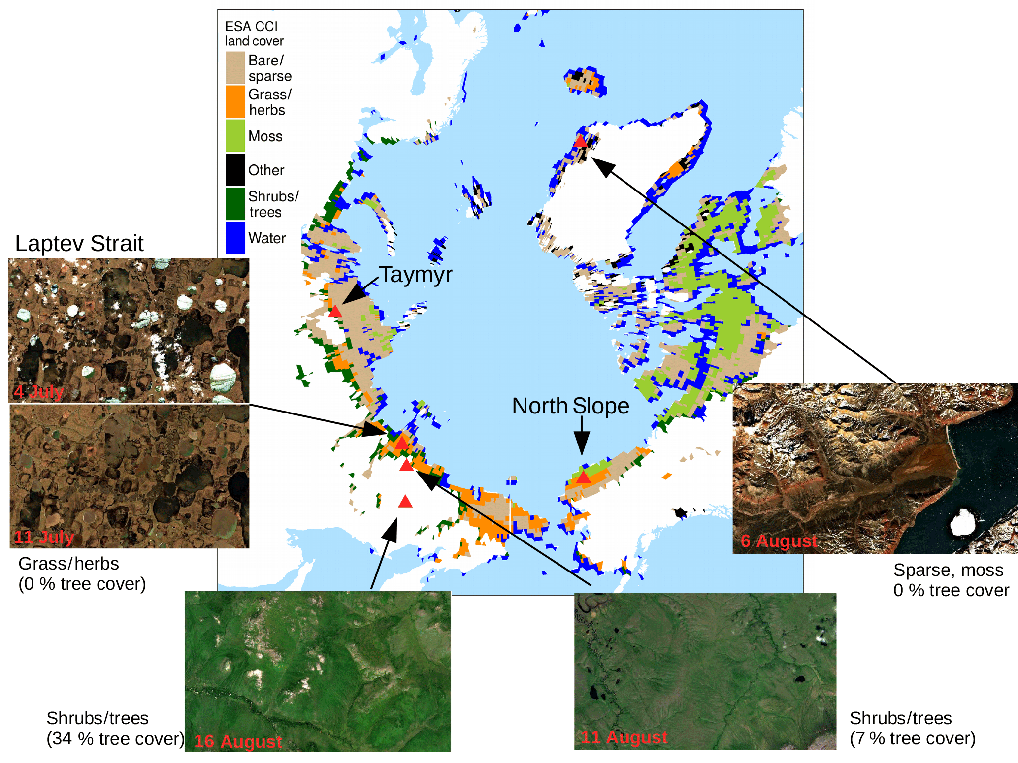
Figure 1ESA CCI land cover in regions with less than 5 % tree cover according to Hansen et al. (2013). Atmospherically corrected true colour images are from Sentinel-2, taken at different dates in 2017. For the region shown in each image the majority land cover is given and the tree cover percentage according to Hansen et al. (2013).
2.2.6 Land cover
We use the ESA CCI land-cover classification and aggregate it to the broader classes of mossy, bare/sparse, grassy/herbaceous, woody, water covered and others. The ESA CCI provides a tool to convert discrete land-cover classes to continuous vegetation fractions (Poulter et al., 2015), and we use it to obtain land-cover fractions from the native 300 m pixels in 0.5∘ pixels for the period 2008–2012 (Fig. A1 in Appendix A). The distribution of moss in these products is expected to be problematic, because it is a complicated class to characterise in terms of global land-cover products. Being partly based on regional maps with varying thematic detail in their legends, it is possible that this moss class in the ESA CCI is not always accurately identified over certain regions, explaining why moss cover is barely indicated in Siberia.
2.2.7 Eddy-covariance-derived GPP
We use eddy-covariance measurements from a subset of the FLUXNET2015 data (http://fluxnet.fluxdata.org/, last access: 29 July 2018; please note that FLUXCOM has been trained on the earlier La Thuile dataset). We chose sites based on data availability after 2007, situated north of 55∘ and that were not characterised as forests (details on sites and site-years used are provided in Table A1 in Appendix A). We use the daily GPP derived using night-time (NT) and daytime (DT) partitioning and aggregate it to 16 day-averages, masking out those days where less than 80 % of reliable measured and gap-filled NEE values were available (with variable Ustar threshold and reference selected on the basis of the model efficiency). Site-level air temperature (consolidated by ERA-Interim and the MDS algorithm) was filtered for good quality and gap-filling in the same way.
We also include the daily GPP derived from NEE by night-time partitioning (Reichstein et al., 2005) from measurements in Cherskiy, Russia (control site RU-Ch2; data courtesy Mathias Göckede, Max-Planck-Institute for Biogeochemistry, Jena, Germany), where only days are used in the average with short data gaps filled (less than 1 day).
2.3 The study area
Operational satellite-derived land-cover data sets exhibit substantial differences in the classes they assign to circumpolar regions. We compared the ESA CCI land cover, GlobeLand30 by Chen et al. (2015) and the IGBP classification from MODIS MCD12C1 and found that the classification of the same area can range from barren to grasslands to open shrub lands depending on the chosen data set (not shown). A clear and generally accepted delineation of a class “tundra” is not given. We therefore define our study area based on tree cover as “polar treeless regions”.
Global data on annual forest cover gain and loss have been provided by Hansen et al. (2013) based on Landsat images. We take 2009 as representative of the period of investigation. Based on information on the global tree cover in 2000, the yearly losses until 2009 and the gains until 2009 (assuming that the growth between 2000 and 2012 that is given in the data set is linear), global tree cover in 2009 is estimated. We aggregated from the original 30 arcsec resolution to 0.5∘. Regions with less than 5 % tree cover north of 55∘ N are fixed as our study area (cf. Fig. 1). In the data from Hansen et al. (2013), a tree is defined to have a minimum height of 5 m, which is tall for circumpolar areas. The studied area will therefore include parts of the taiga–tundra transition zone, tundra and polar deserts.
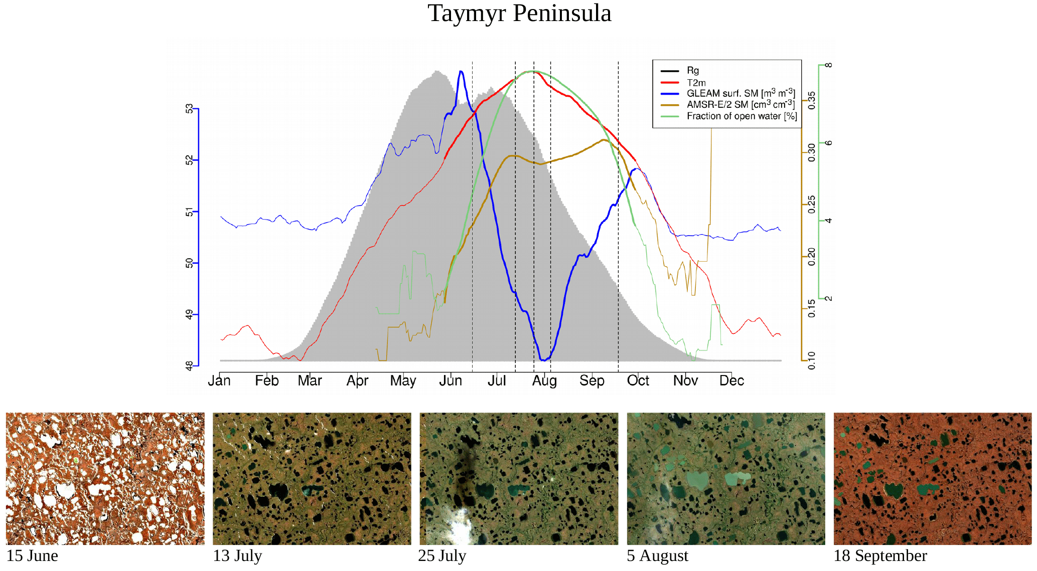
Figure 2Climatologies of different atmospheric and land surface variables for a small area on the Taymyr Peninsula in Russia, indicated in Fig. 1. Bold lines indicate the time period when air temperatures are above the freezing point (no axes displayed for temperature and incoming radiation). Vertical dashed lines indicate the time of the year when the Sentinel-2 images shown in the second panel were taken. Sentinel-2 images are atmospherically corrected and taken in 2017.
The landscape in this study area exhibits a complex microtopography caused by polygons and is characterised by abundant (thaw) lakes. Though vegetation often fully covers the ground (Stow et al., 2004), vascular plant cover is sparse and the growing season and carbon uptake period, consisting of 1 to 3 months, are short in high-latitude tundra. The RGB images from Sentinel-2 for selected spots in Fig. 1 give examples of what tundra landscapes and the tundra–taiga transition can look like. Further, for small areas on the Alaska North Slope and at the bottom of the Taymyr Peninsula (the corresponding places are indicated in Fig. 1), Figs. 2 and 3 illustrate the mean annual cycles of environmental conditions along with Sentinel-2 images at given points in time during the growing season. Temperatures rise above the zero degree Celsius line in late May, and snow melt is often only completed in June. The soil moisture modelled by GLEAM is usually highest at the time of the start of the growing season and illumination is also close to its maximum. Temperatures keep increasing until July (ice layers on lakes can persist until July, cf. Fig. 1, example of the tundra close to the Laptev Strait). GLEAM soil moisture is lowest at the time of highest temperatures, while areas of open water are largest. Light conditions are already diminishing. Temperatures fall below the freezing point in late September to October. During this short period of favourable growing conditions vegetation phenology rapidly develops (Arneth et al., 2006).
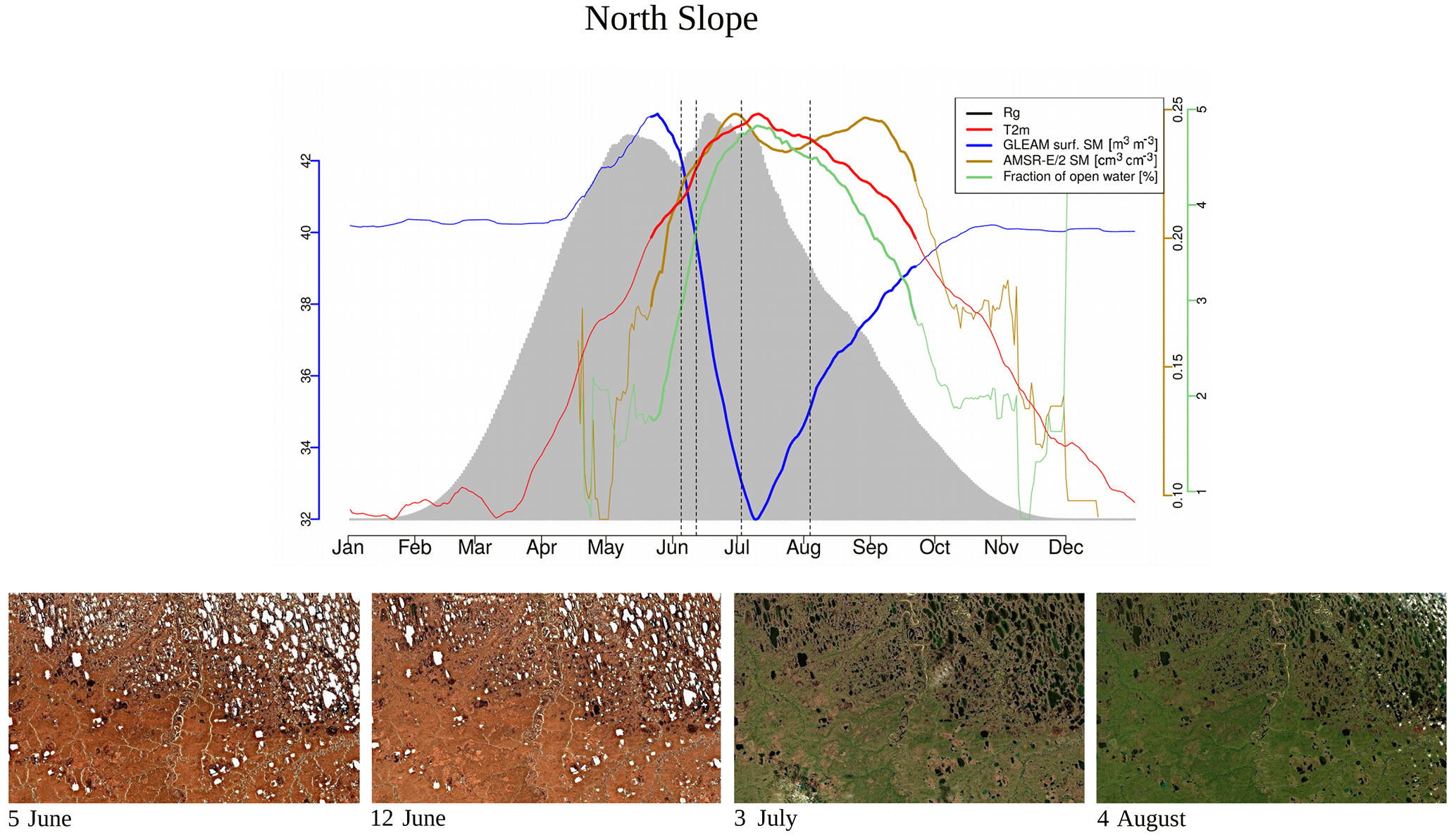
Figure 3Climatologies of different atmospheric and land surface variables for a small area in the North Slope in Alaska, indicated in Fig. 1. Bold lines indicate the time period when air temperatures are above the freezing point (no axes displayed for temperature and incoming radiation). Vertical dashed lines indicate the time of the year when the Sentinel-2 images shown in the second panel were taken. Sentinel-2 images are atmospherically corrected and taken in 2017.
For the evaluation of soil moisture we will focus the analysis on GLEAM data. GLEAM and AMSR-E/2 data on soil moisture partly show different qualitative behaviour (Figs. 2, 3, while they are more similar qualitatively in additional examples in Fig. A2 middle and bottom panel). Possible explanations might include the following: (1) Both refer to slightly different quantities. AMSR-E/2 denotes the volumetric soil moisture in the uppermost 1 cm of land surface while GLEAM refers to surface-soil moisture (denoted as 0-10 cm depth). Full comparability might thus not be given. (2) The applicability of GLEAM data for high latitudes has not been shown. (3) The fraction of open water from AMSR-E/2 shows surprising behaviour, in that we expected the annual maximum to appear in early summer and not very late in the summer. In the examples above of different behaviour in the GLEAM and AMSR-E/2 soil moisture, the latter shows similarly unexpected behaviour. This is indicative of the problems that still need to be faced for soil moisture retrievals in the high latitudes. (4) It is actually not clear what these quantities mean in tundra ecosystems. The microwave signal from the persistently wet peat base of the moss layer can penetrate the dry moss layers (which might reach a thickness of tens of centimetres), but the signal in GLEAM in similar cases is unclear.

Figure 4Distribution of the DOY of the peak of the different vegetation proxies over the study region and between years (spatial sampling matched between data sets for each year). Bars in the boxes indicate the median, stars indicate the mean and the numbers below the bars denote the spatiotemporal mean (standard deviation). Colours of the bars denote grouping of the different variables according to the families of fAPAR, APAR, the modelled GPP, SIF and VOD.
3.1 Timing of the annual peak in vegetation activity and greenness
The distribution of the timing of the annual maximum in polar treeless regions (Fig. 4, regionally and over years) shows a distinct order of the satellite vegetation proxies. All proxies indicate the highest plant activity and biomass after the summer solstice. While APAR is highest around DOY191 (10 July), the METGPP indicates the maximum photosynthetic activity at a similar time and the RSGPP 4 days later. It is the time when surface-soil moisture is almost at minimum, according to GLEAM (Fig. A3). The SIF GFZ peaks only about 1 week later (4 days later in the case of SIF.daily.int GFZ) around DOY202 (21 July). The observations show that the SIF GFZ peak, potentially indicative of the highest photosynthesis, is reached in close synchrony with the annual temperature peak. In fact, SIF GFZ is the only variable whose distribution of the peak timing is not significantly different from the one of temperature (paired two-sided t-test, significance level of 5 %). On average, the SIF NASA peaks only on 28 July (DOY 209), a similar time to when surface inundation through open water is highest (Fig. A3, although both the SIF NASA and AMSR-E/2 data indicate a large range). Removing the effect of incoming radiation from the SIF measurement by dividing by cos(sun zenith angle) shifts the annual maximum for SIF.cosSZA GFZ by 6 days compared to SIF GFZ and by 11 days for SIF.cosSZA NASA compared to SIF NASA, and there is comparatively large scatter. The yearly maximum in vegetation indices occurs in late July to early August, where EVI and NIRv peak at around 31 July (DOY212), 1.5 weeks after the temperature and SIF GFZ maxima. On average, the VOD peaks in close temporal agreement with EVI and NIRv. Finally, up to 5 days later the MODIS VIproduct as well the NDVI reach their maxima in the first week of August. Statistically, the NDVI peak timing is significantly different from the one of all other vegetation proxies (paired two-sided t-test, 5 %). The scatter between years and regions (standard deviation) is smallest for the modelled GPP data, where the RS set-up interestingly shows a larger spread. APAR and the vegetation indices based on MCD43C4 have standard deviations of 12 to 14 days, slightly smaller than those of the MODIS VIproducts and of the SIF GFZ data sets (17 to 20 days). The largest uncertainties are shown by the SIF NASA data sets and the VOD. Still, grouping indicators based on the similarity of their intrinsic properties (e.g. RSGPP and METGPP, SIF GFZ and SIF NASA, EVI, and NIRv) shows that such groups have a consistent behaviour and follow a certain pattern; APAR indices < modelled GPP < SIF < fAPAR (with EVI, NIRv, VOD < NDVI).
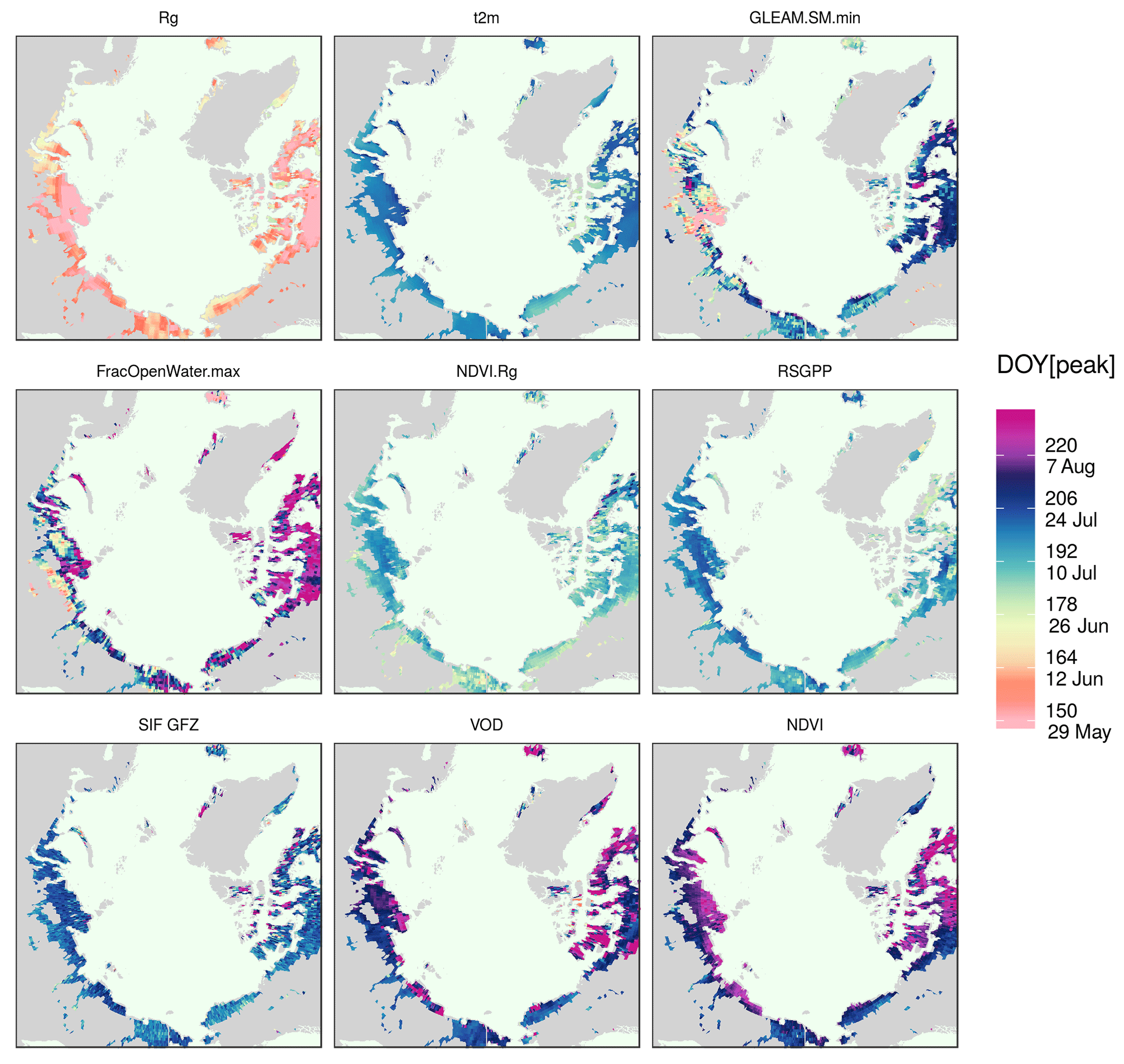
Figure 5DOY of the annual maximum averaged over all years, as indicated by selected vegetation proxies.
3.2 Spatial patterns of the annual maxima of the satellite vegetation proxies and of the lags between them
There is considerable spatial variability in the timing of the maximum for each satellite indicator (Fig. 5). In areas close to the Date Line (i.e. easternmost Siberia and Alaska), most proxies peak slightly earlier than in northern Canada (mainland and islands) or the coasts of western and central Siberia (i.e. Taymyr Peninsula and regions of the Lena delta and the Laptev Strait). In general, the spatial pattern of the timing of the annual maximum of the satellite indicators closely corresponds qualitatively to the dynamics seen in air temperature and partly in the surface-soil moisture (GLEAM). Incoming light shows partly reversed patterns with an earlier maximum irradiance in northern Canada and western-central Siberia.

Figure 6Average time difference of the maximum across years of selected vegetation proxies and the NDVI.
We test whether the annual maximum is shifted systematically or whether there are spatial gradients in the peak lag between proxies and plot maps of the average lag between the peaks of selected proxies and NDVI. We take the NDVI because it is the most widely used vegetation index for productivity studies, both from the satellite as well as in ground-based observations, particularly in the polar tundra. Figure 6 confirms the general pattern of a shifted annual peak of NDVI as compared to NDVI.Rg, RSGPP, SIF GFZ, VOD and the similar timing to EVI over the entire study area. The NDVI.Rg, RSGPP, SIF GFZ, VOD and air temperature reach their annual maxima at significantly different times than the NDVI (Fig. A4). Figure 6 further shows that the lag is not homogeneous in space, but that it is largest in vast areas of polar desert in northern Canada, on Iceland and in the northern part of the Siberian Taymyr Peninsula. Interestingly, the tundra regions that exhibit the largest time difference of the annual maximum between the individual vegetation proxies and NDVI tend to correspond to those where the annual maximum is reached comparatively late (Fig. 5). In contrast to the denser vegetation cover on the Siberian coast, very sparse vegetation (i.e. devoid of shrubs or woody vegetation) characterises the northern Canadian regions, both the islands and the mainland as well as the northern part of the Taymyr Peninsula (cf. Fig. A1; Walker et al., 2005, their Fig. 1). In addition, there is a comparatively high amount of lakes and a high fraction of barren regions in the areas of large NDVI lags in the central Siberian coastal areas (close to the Laptev Strait), coastal Alaska North Slope and in mainland Canada northwest of Hudson Bay. Similar results are obtained for EVI.Rg, METGPP, SIF.daily.int GFZ (Fig. A5). Next to these general observations, the VOD indicates a much later peak in smaller but contiguous areas in northwestern Canada as well as in the lake-rich regions on the Siberian coast (again the coast close to the Laptev Strait). The NDVI lags to METGPP are generally slightly larger than those to the RSGPP. No outstanding region emerges for the lags when compared to SIF NASA. The illumination correction of SIF (SIF.cosSZA) reduces the time difference to the NDVI when compared to the instantaneous SIF, as expected.
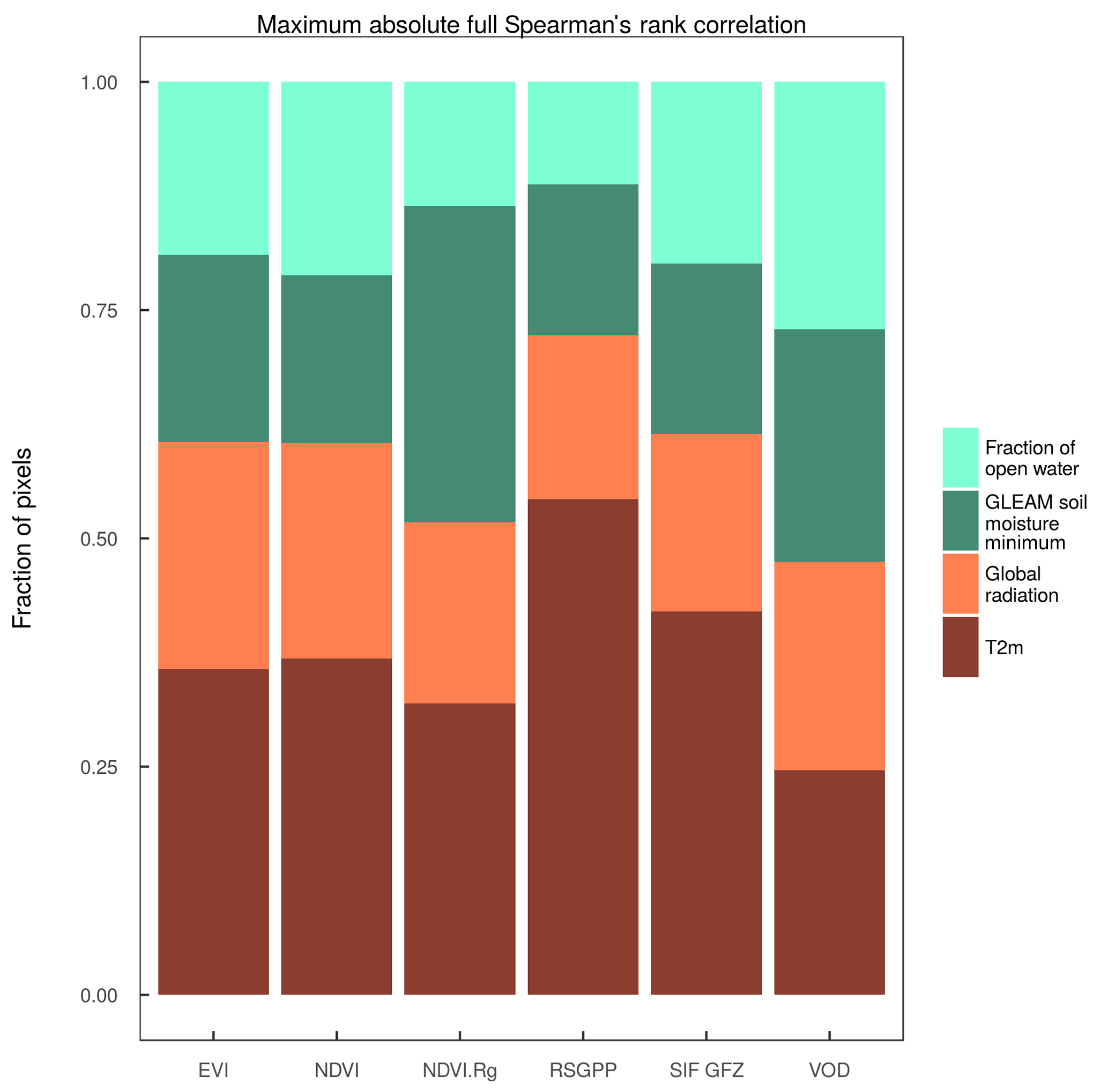
Figure 7Frequency distribution of the pixel-wise Spearman's rank correlation between the peak DOY of the vegetation proxies across years and the peak DOY of environmental variables in spatial moving windows of 1.5∘ (9 spatial pixels times 10 years at most, correlated only if more than 20 data points available). Plotted here is the variable with the highest absolute correlation without the filter for statistical significance. Full correlations have been calculated (no partial correlations).
3.3 Spatial patterns of peak timing and of peak lags to the NDVI in relation to environmental variables
Putting the annual maximum of the NDVI into relation with that of the environmental variables, partially similar spatial patterns to the vegetation proxies emerge (Fig. 6). More precisely, air temperature and soil moisture (GLEAM minimum) peak earlier everywhere and have the largest time difference to the NDVI in the sparsely vegetated areas on Iceland, northern Canada and parts of the Taymyr. Conversely, for the microwave retrievals of the amount of open water on the surface, mixed temporal relationships with the NDVI peak are observed. Most of the water mapped from microwave remote sensing is present after the time of NDVI peak in large parts of northern Canada, Greenland and inland masses close to the Date Line, while the NDVI is at its maximum after the fraction of open water in all other regions. Summer precipitation might increase surface wetness and influence the microwave fraction of open water, as the highest surface inundation is typically expected to happen immediately after snow melt.
It is further interesting to test whether a certain temporal relationship between the maximum in photosynthesis or greenness and the dynamics of the environmental conditions holds across years. In Fig. 7, the environmental variable with the highest absolute value of the rank correlation, with the timing of the maximum of the given satellite proxy across years in a spatial moving window, is displayed. The important role of energy-related variables for vegetation activity and growth, mostly temperature, is highlighted by the highest widespread correlations with temperature and radiation for RSGPP, SIF GFZ, EVI and NDVI, while moisture-related variables are most important only in about one third of the pixels. The VOD and NDVI.Rg do show a strong relationship, with the annual temperature maximum only in 25 % to 30 % of the pixels and about half of the pixels show a higher importance of soil moisture or open water on the surface. It is worth noting that the contiguous regions with higher relationships with moisture-related variables for RSGPP, EVI and NDVI are situated in northwestern Canada and parts of the Taymyr (Fig. A6).
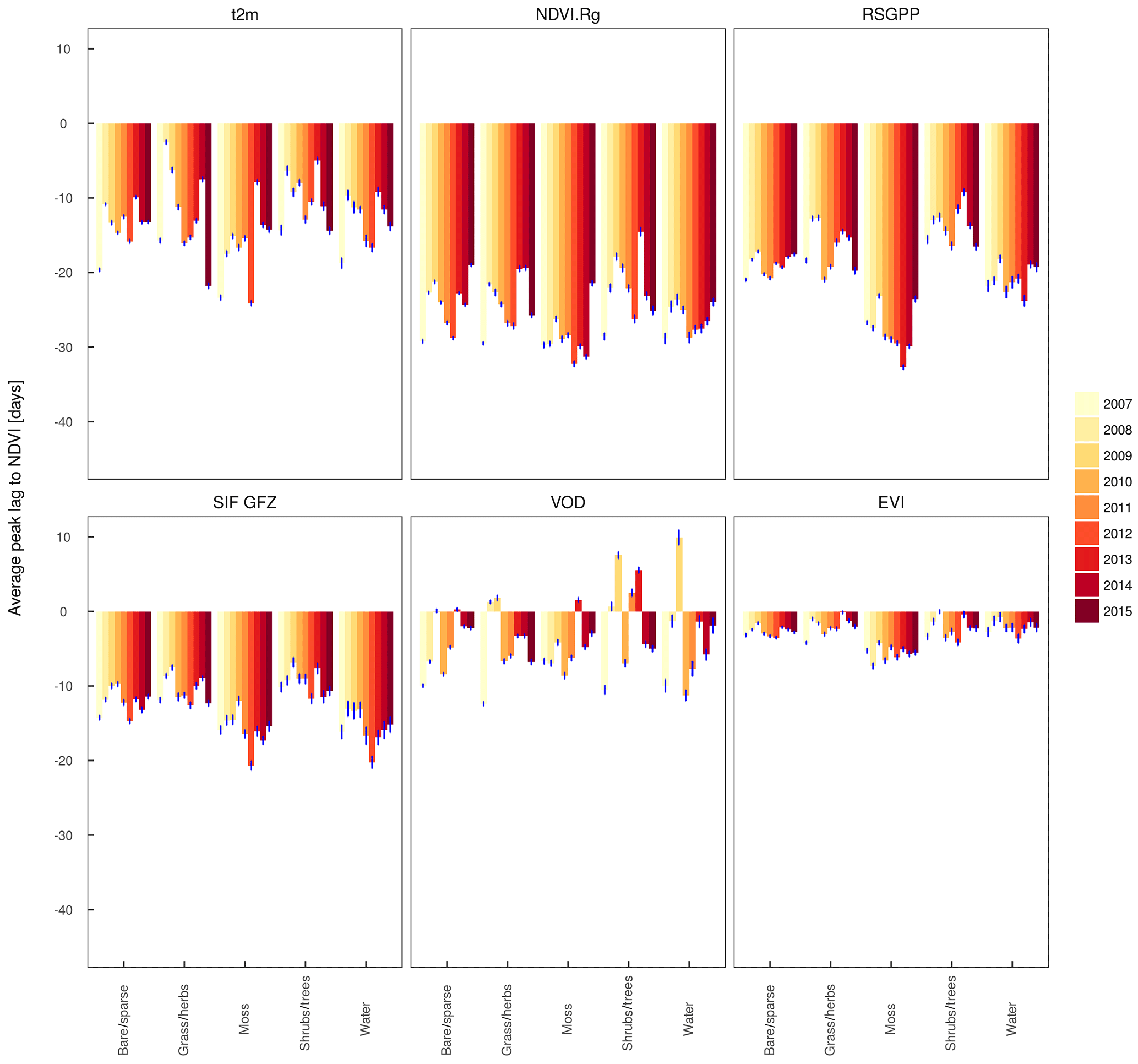
Figure 8Average of the time difference between the peaks of one selected variable per family (APAR, fAPAR, SIF, GPP, VOD) and the NDVI as a reference, weighted with fractional cover per vegetation type (based on ESA CCI) and per year. Each bar represents the average of 50 bootstrap samples of the time series per year, pixel and vegetation proxy; error bars indicate a multiple of 1.96 of the standard deviation across the 50 samples.
Interestingly, apart from the strong correlative relationship of photosynthesis with temperature, the lags in the annual peak timing between the temperature and SIF GFZ (Fig. A7) are barely statistically significant. Peak lags between the RSGPP and temperature are only significant in northern Canada and easternmost Siberia. Conversely, EVI, NDVI, VOD and in the largest parts of the study area also NDVI.Rg, peak at significantly different times in the year than air temperature.
3.4 Consistency of the annual peak lags between different land covers and across years
The fact that there is spatial variability in the shift between the annual peaks of the satellite proxies relative to the NDVI suggests that the proxies differ in how strongly they indicate the spatial gradients in the peak DOY. We test to what extent the shift of the annual maximum holds across different years and whether there is a dependency on the land cover. Figure 8 (and Fig. A8, but here based on the actual time series and not the bootstrapped values) shows the peak lags as a function of land cover based on the ESA CCI for all years in the study period separately. Peak lags to the NDVI per proxy are generally similar between land covers, although there is a tendency in several proxies (excluding the VIproducts of MxD13C1, METGPP, SIF NASA) towards larger lags in regions classified as moss. According to Fig. A1, this largely corresponds to the sparsely vegetated areas in northern Canada, also with high cover fractions of water and barren. The smallest lags of RSGPP and SIF GFZ are shown for the mixed shrub and tree land covers. There is also some variability between years, which is largest for the timing of the moisture-related variables of the maximum extent of open water and the GLEAM soil moisture minimum. Conversely, the variability in the peak lag per land cover is smaller for the vegetation proxies between years. The VOD is maximised 5 to 7 days earlier than the NDVI in tundra-like vegetation types, but it has no consistent relationship with the NDVI in forests and water. Interesting patterns are the large NDVI-t2m lags in 2015 in grass and herb areas and 2012 in mossy areas as well as the particularly small lag in 2013 in mixed shrub and tree areas. This behaviour between years is qualitatively similar to the RSGPP-NDVI and SIF GFZ-NDVI but is rather caused by the variability in the peak timing of temperature than of the NDVI (not shown).
Despite the considerable challenges for remote sensing applications in high latitudes and inherent comparatively large variability in the timing of the annual maximum, the differences in the peak timing of families or groups of key satellite indicators of plant productivity appear to be ordered in the polar tundra. Absorbed energy (APAR, both EVI.Rg and NDVI.Rg) is maximised roughly 1 month after peak irradiance in early July. Regarding the modelled GPP and SIF as indicators of photosynthetic activity, there is a time lag between them of 4 days to 2.5 weeks, depending on the combination of data sets. The modelled GPP peaks at a similar time to APAR. SIF GFZ reaches its maximum 1 to 1.5 weeks after (21 July) at a very similar time to air temperature, but SIF NASA only reaches its maximum at the end of July (DOY 209, 28 July). Greenness (EVI and NIRv) culminates 3 weeks after APAR and 1.5 weeks after SIF GFZ. NDVI maximum is delayed an average of 3 more days. Peak vegetation water content is indicated by the VOD at a similar time as EVI and NIRv. The spread in space and across years is, however, large.
Vegetation activity is highly (though not exclusively) temperature-driven in tundra (Chapin, 1987; May et al., 2017; Stow et al., 2004). In the beginning of the growing season, light is abundant and plants rely on rhizome nutrient and carbohydrate reserves to rapidly increase photosynthetic activity (Arneth et al., 2006) and growth (Chapin, 1987) through exposed moss, lichens and evergreens after snow melt and the rapid leaf-out process of deciduous plants. The fact that the photosynthesis seasonal maximum is reached in close and significant (SIF GFZ and RSGPP) temporal agreement with air temperature adds plausibility to the observed patterns in the modelled GPP and SIF. As the time of favourable environmental conditions for growth is short, several plant types strongly build up their photosynthetic capacity until late in the growing season to make use of the available light and temperature (Rogers et al., 2017). At the time when greenness is at a maximum, photosynthetic rates are decreasing, as PAR is already strongly reduced and the temperature peak has also passed. The peak timing of the SIF before greenness might hence indicate that although photosynthetic potential (fAPAR) is not yet fully developed, plants profit from the higher amounts of light and maximal temperature still present in the year to reach peak photosynthetic rates in the second half of July. The prolonged build-up of photosynthates in plant tissue results in a delayed maximum of green biomass. The widespread agreement between greenness proxies and photosynthesis proxies in high correlation with the temperature maximum across years and space (Fig. 7) are also indicative of the coordinated dynamics of annual maximum photosynthetic activity and the resulting peak photosynthetic potential (fAPAR) with temperature.
The results of Chadburn et al. (2017) support this interpretation of the patterns in the satellite observations. In their site-level evaluation of carbon fluxes in the high latitudes in Earth system models, GPP always depends on temperature but is limited rather by the LAI in the first part of the growing season until the end of July. After that, GPP is more driven by light, which qualitatively agrees with the earlier photosynthesis peak seen in our results. Besides, at the site-level, gas flux measurements show a similar timing of the maximum GPP in the first half of July or mid-July (Emmerton et al., 2016) and at the time of the annual temperature peak (Kross et al., 2014; Welker et al., 2004). This is similar to Lafleur and Humphreys (2008), who report on the largest annual site-level NEE after the summer solstice near the annual temperature maximum between DOYs190–210 and the dominant role of gross ecosystem productivity (GEP) in driving these dynamics.
An interesting aspect of the general time lags between proxies is the 10- to 12-day time difference between peak APAR and peak SIF GFZ. According to the Monteith model for SIF, the observation of a time difference of peak APAR and the peak SIF suggests that SIF might contain information on the temporal dynamics of the actual photosynthetic light-use-efficiency of tundra vegetation. Circum-arctic vegetation is adapted to low light intensities to also allow photosynthesis at low irradiance (Chapin, 1987; Rogers et al., 2017). Consequently, photosynthesis will rapidly become light-saturated, a situation that calls for high levels of non-photochemical quenching in order to avoid photodamage and inhibition by excess energy. Under these conditions, the efficiencies of carbon fixation and fluorescence emission are positively correlated (Porcar-Castell et al., 2014). Consequently, our results indicate a potential benefit of also using SIF in modelling the photosynthetic carbon uptake in the circumpolar tundra for its apparent sensitivity to both APAR and photosynthetic light-use efficiency. Although they did not report on results on GPP, Luus et al. (2017) found higher agreement between the modelled NEE and eddy-covariance-derived NEE when phenology is prescribed by SIF instead of EVI in the tundra in Alaska.
Although the modelled GPP, SIF GFZ and SIF NASA are indicators of photosynthetic activity and they peak closer to the annual temperature maximum than both the APAR and greenness indices, they do differ in peak timing as well. In the following, we test a suite of possible explanations from a physiological decoupling of SIF and GPP to artefacts originating from data processing and data characteristics.
-
The time difference of the yearly maximum of the GPP model and SIF GFZ cannot be fully explained. Since the SIF maximum is reached in close and statistically significant temporal agreement with air temperature, it might indicate that SIF shows a higher sensitivity of photosynthetic rates to temperature. The earlier peak of the modelled GPP might be explained by a possible higher sensitivity to radiation as it is challenging to model the effects of the water table depth and temperature acclimation. This is especially true for the METGPP that culminates slightly earlier than the RSGPP, which is driven by a mean seasonal cycle and greenness that is not temporally resolved. Generally, the model performance of the modelled GPP is reduced in extreme climates (Tramontana et al., 2016). Furthermore, the FLUXCOM GPP might not accurately represent the GPP in tundra due to the small size of training data. The FLUXCOM GPP is trained at the FLUXNET sites and according to Tramontana et al. (2016), there are 11 sites north of 55∘ that are not classified as forest or temperate and serve the modelling of the GPP in our study area. Five of them are located north of 65∘ and the three training sites classified as arctic are all located in Alaska.
We attempted to get an indication of whether – compared to an in situ eddy-covariance-derived GPP and site-level temperature – there is a systematic shift of either the modelled GPP (for the 0.5∘ grid box whose centre coordinates are closest to the flux tower) or the SIF GFZ (16-day averages of all GOME-2 footprints with centre coordinates within a radius of 30 km from the flux tower). Such comparisons of satellite observations with site-level measurements can be very helpful for the interpretation of the patterns seen from space, but here they remain inconclusive. There is agreement between the site-level and regional analyses with respect to the order of the modelled GPP before temperature, but the order regarding the time of the peak SIF GFZ and temperature is reversed (SIF GFZ earlier at the site level, but after temperature at the regional scale, Figs. A9, A10). The comparison is hampered by a number of issues, including the (i) mismatch of scale and spatial representativeness, (ii) limited temporal overlap of site data with satellite records, (iii) data quality of the NEE and temperature at the site level (e.g. Figs. A11–A14), and (iv) quality of partitioning at the site level (Parazoo et al., 2018; Runkle et al., 2013), (v) temporal scale of daily integrated EC measurements and instantaneous SIF observations in the morning (Parazoo et al., 2018). These issues clearly suggest that EC cannot always be used as the “truth” in evaluating satellite observations. At the same time these results strongly underline the observational problems in the tundra explained in the introduction and call for more in situ measurements that are well characterised and understood in order to interpret the signals seen from the satellite.
As we do not find a physiological explanation, artefacts in SIF might originate from seasonal cloud cover as well as from satellite over-pass time and explain the time difference in the annual peak between the modelled GPP and SIF GFZ. Clouds affect the SIF values, both physiologically at the leaf level and on its way from the canopy to the satellite. A possible bias of rather clear-sky instantaneous observations of SIF in the morning hours compared to the modelled GPP, which is an all-day measure, might occur (Parazoo et al., 2018). Although there have been no tests in tundra, in both model simulations (Frankenberg et al., 2012) and empirical analyses (Köhler et al., 2015) choosing different thresholds of cloud cover does not strongly affect temporal patterns of SIF, and a large fraction can still be detected in moderately thick clouds. In our tests (Fig. A15), stricter cloud filters tend to slightly enlarge the lag between the modelled GPP and SIF GFZ, while SIF NASA shows no change. Conversely, SIF GFZ peak time shows no sensitivity to over-pass time, while in SIF NASA, noon over passes indicate a slightly earlier peak than using measurements between 08:00 and 14:00 LST Although data availability becomes problematic in the case of OCO-2, resulting in discontinuous climatologies, there is mostly agreement with OCO-2 SIF when averaged from larger regions (Fig. A17). This suggests that the peak timing obtained from GOME-2 SIF GFZ observations is reliable.
-
There is also a relatively large inconsistency between SIF GFZ and SIF NASA. We conducted tests in which we strictly filtered for the same cloud fractions (0.3) and over-pass times (08:00–14:00 LST) in both data sets. We did not attempt a one-to-one allocation of individual soundings between data sets, and it must be noted that the cloud fraction is defined in a slightly different way between SIF GFZ and SIF NASA (see methods). Indeed, a stricter cloud filter of 0.3 instead of 0.5 delays the SIF GFZ peak slightly, bringing it into closer to but not reaching a full temporal agreement with the SIF NASA peak (Fig. A15). Strict filtering for midday over pass times advances (Parazoo et al., 2018) the annual peak, but for other combinations of over-pass filters no systematics appear.
We argue that the NASA data set is more prone to noise (for example, for retrievals over bright surfaces when there is partial snow cover) due to the generally lower absolute values that result from a narrower retrieval window and that this severely affects the identification of the annual peak. This is indicated by the large spread in Fig. 4, by the less pronounced spatial patterns in Fig. 6 and by the time series examples in Fig. A16. Further, the illumination correction amplifies noise in the time series. This is thus an example for the degradation of the signal by the division by cos(SZA) and calls for caution in applying it. We conclude that the different cloud fractions can explain a part of the difference between the SIF GFZ and SIF NASA and argue that the remaining difference might be ascribed to the different noise levels in the two data sets that make a reliable peak identification in SIF NASA more difficult than in SIF GFZ and also lead to a larger spread.
In our results, the NDVI and the MODIS VIproducts are the latest greenness proxies and peak around DOY216 (4 August). The NDVI is a widely used indicator of productivity, and a comparison to both ground-based measurements and satellite observations with the AVHRR instrument shows mostly support for the NDVI peak in very late July or the beginning of August. The ground NDVI along a transect in Alaska by Stow et al. (2004) and Stow et al. (2004) agree with the MODIS NDVI in that the seasonal maximum is observed at DOY218 in the beginning of August. In a second year there is even a second peak at DOY230 in the ground-based NDVI. Huemmrich et al. (2010a) show a time series of ground-based NDVI in Alaska that reaches the peak about 2 weeks earlier (at DOY203) than the average MODIS NDVI in our results but remains high until the end of August. However, May et al. (2017) report on peak dates of in situ measured NDVI in Alaska roughly 1 week to 2 weeks earlier (DOY 199-207) and talk about the beginning of senescence after the first sunset in late July to the beginning of August. Finally, the satellite-based biweekly NDVI from the AVHRR instrument is shown to peak between 22 July and 4 August (Stow et al., 2004; Zhou et al., 2001). Still, the onset and the peak timing of MODIS-based NDVI have also been found to be inconsistent with ground-based observations of NDVI (Gamon et al., 2013), which might suggest partly questionable reliability of satellite NDVI.
While the reported ground observations were all conducted in Alaska, in our circumpolar results the NDVI largely agrees with the other vegetation indices of the EVI and NIRv, only peaking later in the north-easternmost parts of Canada (Figs. 6 and A5). In addition to the Taymyr and coastal North Slope Alaska, these are the same regions where the NDVI lags to all other proxies are also largest. According to the ESA CCI land cover, those regions are characterised by moss (Fig. 1). Moss often has no clear seasonal cycle of greenness, making a peak identification difficult. Moreover, vegetation is particularly sparse in the form of prostrate dwarf shrubs, and there are extensive barren areas with rich lake cover in those northern Canadian areas (Walker et al., 2005). This renders the reflectance-based observation particularly sensitive to background conditions, especially without a clear seasonality in greenness (Walker et al., 2005). Confirmation for this hypothesis of the strong contamination of the NDVI signal is given by the sharp transition from the very large lags in northeastern mainland Canada (eastern Barren Grounds) to lower albeit still negative lags to the northwestern part of mainland Canada (Fig. 6 and A5, corresponding to the land-cover transition between bare and sparse in the western parts of the Barren Grounds to moss in the more easterly regions of the Barren Grounds in Fig. 1). Similar to the northern Canadian islands and northeastern mainland, northwestern Canada is characterised by many lakes (Walker et al., 2005), and the ESA CCI land-cover reports sparse vegetation with much moss and open water as well (Fig. A1). However, in these more western areas, vegetation changes to erect dwarf shrubs and graminoids instead (Walker et al., 2005), which exhibit a clearer seasonality (Fig. A18, panel of northwestern Canada) than the very sparse vegetation in the eastern parts with prostrate shrubs (Fig. A18, northern mainland and islands of the Canadian Arctic Archipelago, northeastern Canada and Iceland). These are also less affected by increasing values at the beginning and at the end of the growing season that are even partially higher than the summer maximum, severely influencing the identification of the annual peak. We speculate that possible explanations for this might be an increasing effect of low SZA late in the growing season (Kobayashi et al., 2016), affecting low NDVI in particularly sparse vegetation heavily. The NDVI might also be strongly decreased by standing surface water (Gamon et al., 2013) from snow melt or intermittent precipitation that has not yet drained or evaporated until later in the growing season. Only upon drying will the NDVI increase due to the missing water absorption in the near infrared, and this might most strongly affect the trajectory of the NDVI in the sparsely vegetated regions with the largest peak lags.
The highest vegetation water content is indicated by the VOD at a very similar time to the peak values of the vegetation indices, which might corroborate the usefulness of VOD to indicate vegetation biomass in tundra ecosystems, too. Both vegetation indices and the VOD are sensitive to vegetation structure and density and VOD in addition to water content (Liu et al., 2011). Especially in low biomass regions – as applied for tundra – a linear relationship between the VOD and vegetation water content has been found (Teubner et al., 2018). The similarity of the VOD as an indicator of total aboveground biomass to the vegetation indices might also support our interpretation of delayed peak greenness compared to photosynthesis, which is due to the longer-lasting allocation of plant material and pigments and indicate that the proposed relationship by Teubner et al. (2018) between the VOD, vegetation water content, LAI and GPP does not fully hold in the tundra. Conversely, when looking at examples of the mean seasonality of the VOD in comparison to the other vegetation proxies for selected regions (Fig. A19), the VOD annual cycle appears broader and the peak less well defined than the one of the vegetation indices. This could indicate that the vegetation water content changes only slightly during the growing season, while the chlorophyll concentrations possibly independently exhibit more pronounced dynamics and affect the vegetation indices to a greater degree. Another possible factor contributing to the broader annual cycle is the VOD's relation to the water content of the total aboveground biomass (as opposed to green or photosynthetic biomass), including moss, woody components and litter. If persistently wet, moss might drive the VOD signal and the greenness signal, though to a lesser degree. There is a high sensitivity of moss to air humidity as a consequence of the absence of roots. Despite a wet peat layer, there might be several centimetres of dry moss material. In grassy land, consistently high emissions and a consequently lower VOD seasonality were ascribed to the contributions of litter and wet vegetation components (Grant et al., 2016). Similar mechanisms might also hold for the VOD observations in tundra, especially considering that carbon turnover is slow in the high latitudes. It is also not clear what the VOD signal on water saturated soil might be. Moreover, the retrieval of the VOD is strongly dependent on the representation of open water and soil moisture. Considering that the retrieval algorithms have not been calibrated for tundra-like conditions and that with the high heterogeneity regarding plant types and landscape components, it might be difficult to accurately separate the contributions of vegetation from soil and water, it is not clear what the VOD in tundra means. In future studies it would be useful to analyse a suite of different VOD products from different sensors and wavelengths along with in situ observations in order to understand whether greenness and vegetation water content are strongly coupled in tundra or not and to what extent different retrievals affect the results.
Overall it must be stated that gaps in the data and the short growing season with often small seasonality and high noise levels challenge the reliable identification of phenological dates in all data sets.
We analysed and compared satellite-based indicators of plant productivity with respect to the timing of their maximum in arctic treeless regions. Over the whole study area, peak productivity is generally reached in July with an order of APAR, culminating in the first half of July along with the modelled GPP and followed by SIF GFZ one week later in synchrony with the highest annual temperatures. SIF NASA is delayed by 1 week. The EVI and NIRv indicate maximum greenness in the end of July, along with VOD as a proxy for vegetation water content. NDVI and MODIS VIproducts peak only in the first week of August. We interpret this sequence as the growth and synthesis of leaf tissue and pigments even after optimal conditions for assimilation regarding light and temperature have passed. Peak photosynthesis occurs earlier, at a time when full photosynthetic potential has not yet developed but when light is still abundant and the temperature favourable. The largest lags between the NDVI and photosynthesis indicators are found in regions with particularly sparse vegetation and without a clear seasonality in spectral reflectance that can heavily be confounded by low sun angles and the high abundance of lakes.
To our knowledge, only few studies of tundra vegetation have been based on other variables observed than spectral reflectance (Luus et al., 2017; Parazoo et al., 2018). It was questioned a priori whether current satellite-based SIF data sets are useful for tundra vegetation considering the very large footprints, high susceptibility to noise and very small signals from the sparse vegetation. However, the spatial patterns of peak productivity of SIF are qualitatively similar to the ones seen in the modelled GPP and reflectance-based observations. Furthermore, the fact that the SIF maximum is reached in close temporal agreement with air temperature might indicate a benefit for photosynthesis from the highest temperatures. The general time difference between the proxies of APAR and SIF suggest that there is information on light-use-efficiency contained in the SIF observations. Still, further studies are needed to verify this. The results of our study confirm the important separation between indicators of greenness and photosynthesis and also highlight non-negligible differences between data sets of the same indicators. Regarding data availability in the future, similar cross comparisons to the chlorophyll–carotenoid index (Gamon et al., 2016) and the photochemical reflectance index (Gamon et al., 1992) in tundra might still add additional complementary information on circumpolar vegetation dynamics.
Code and data available upon request.
Averaged over all sites and years (Fig. A9), site-GPP peaks about 10 days earlier than site-level air temperature, with both partitioning and the quality filter shifting the peak time up to 5 days. Time lags of very similar magnitudes are shown by the grid-cell modelled GPP. In this respect the patterns at the site level agree with the slightly earlier GPP-model peak, compared to the temperature peak seen in the regional and interannual analyses (Fig. 4). Conversely, while in the large-scale pattern, SIF GFZ and SIF NASA peak close to but slightly later than the air temperature; at the site level, SIF GFZ indicates a maximum at a similar time to the modelled GPP and the EC-derived GPP (excluding spurious results from sites NO-Adv, DK-ZaF and DK-ZaH, where strong differences between the partitionings are apparent and/or an annual cycle in the SIF data are absent; Fig. A12) and peaks before air temperature.

Figure A1Fractions of the aggregated land-cover classes for the ESA CCI land-cover data set. The aggregated classes comprise “moss” (class 100 in the ESA CCI classification), “bare/sparse” (classes 28–30, 35–37, fractions of 16 and 19), “grass/herbaceous” (classes 26, fractions of 13, 16, 19, 21–25, 33), “woody” (shrubs and trees, classes 10–12, 14, 15, 17, 18, 20, fractions of 13, 16, 19, 21–25, 31–33), “water” (class 38, fractions of 31–33) and “other” (remaining classes and fractions).
For individual sites the patterns are less clear. Despite a frequent tendency for an earlier peak of the EC-GPP, the signs of the time lags between the peak EC-GPP and temperature are not consistent. For NO-Adv, RU-Cok, RU-Sam and SE-St1, partially strong dependencies of the peak DOY on the partitioning method and the quality filter are seen. The modelled GPP is maximised somewhat earlier than the site-level temperature, and at some sites the lags become very small. For the sites where the SIF time series show a growing season and not pure noise, which excludes DK-ZaF, DK-ZaH (Fig. A12) and NO-Adv, SIF GFZ reaches its maximum earlier on average than the site-level temperature, although there is a large spread in the magnitude of the lag of 3 to 26 days between sites.
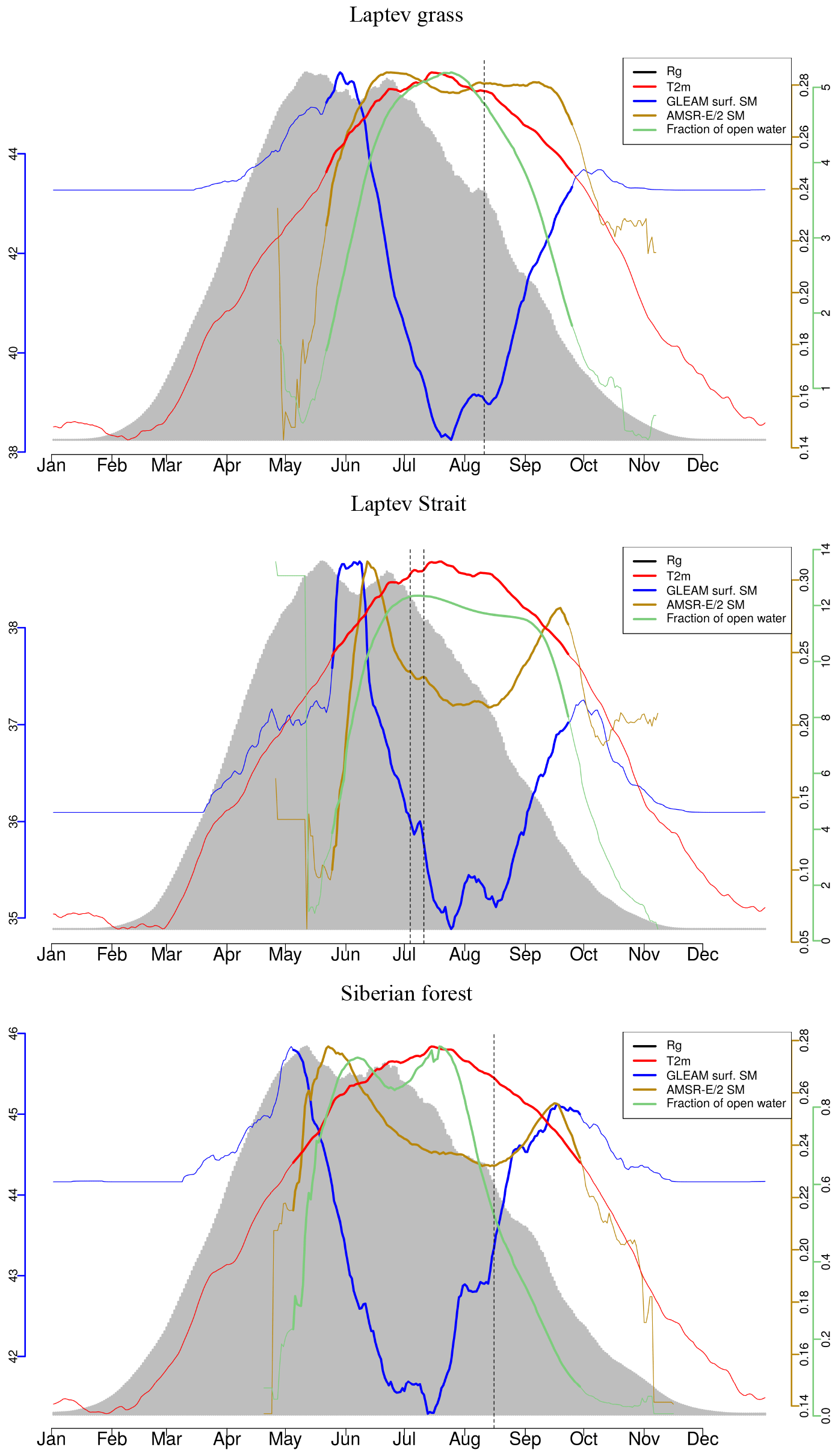
Figure A2Climatologies of different atmospheric and land surface variables for different small area indicated in Fig. 1. Bold lines indicate the time period when air temperatures are above the freezing point (no axes displayed for temperature and incoming radiation).
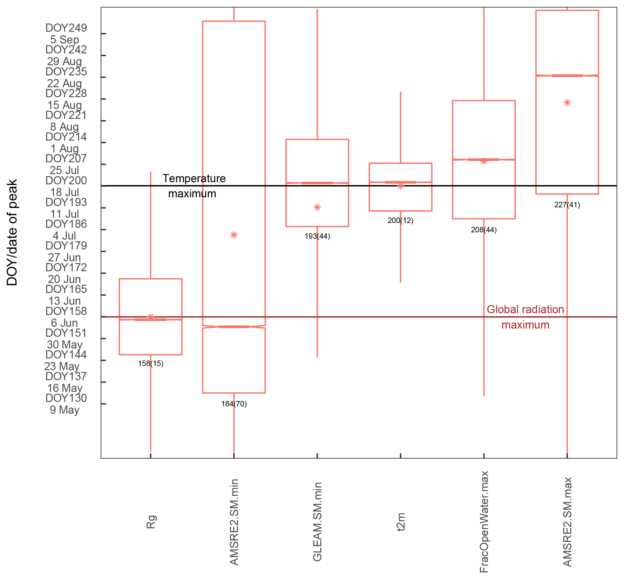
Figure A3Distribution of the DOY of the peak of the different environmental variables over the study region and between years (spatial sampling matched between data sets for each year). Bars in the boxes indicate the median, stars indicate the mean and the numbers below the bars denote the spatial mean (standard deviation).
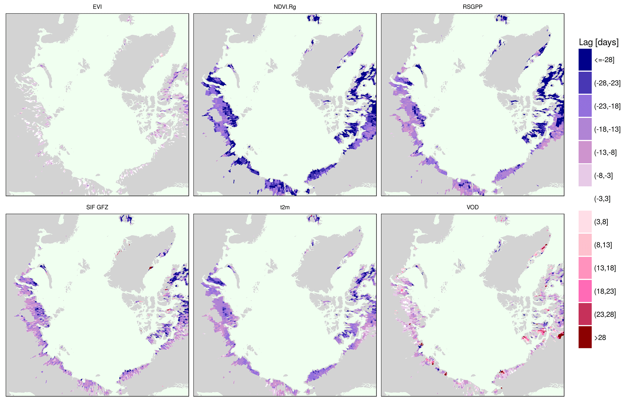
Figure A4Average time difference of the yearly maximum across years between selected vegetation proxies and the NDVI based on 50 bootstrap samples of each year's time series. Shown are only statistically significant differences at a level of 5 %.
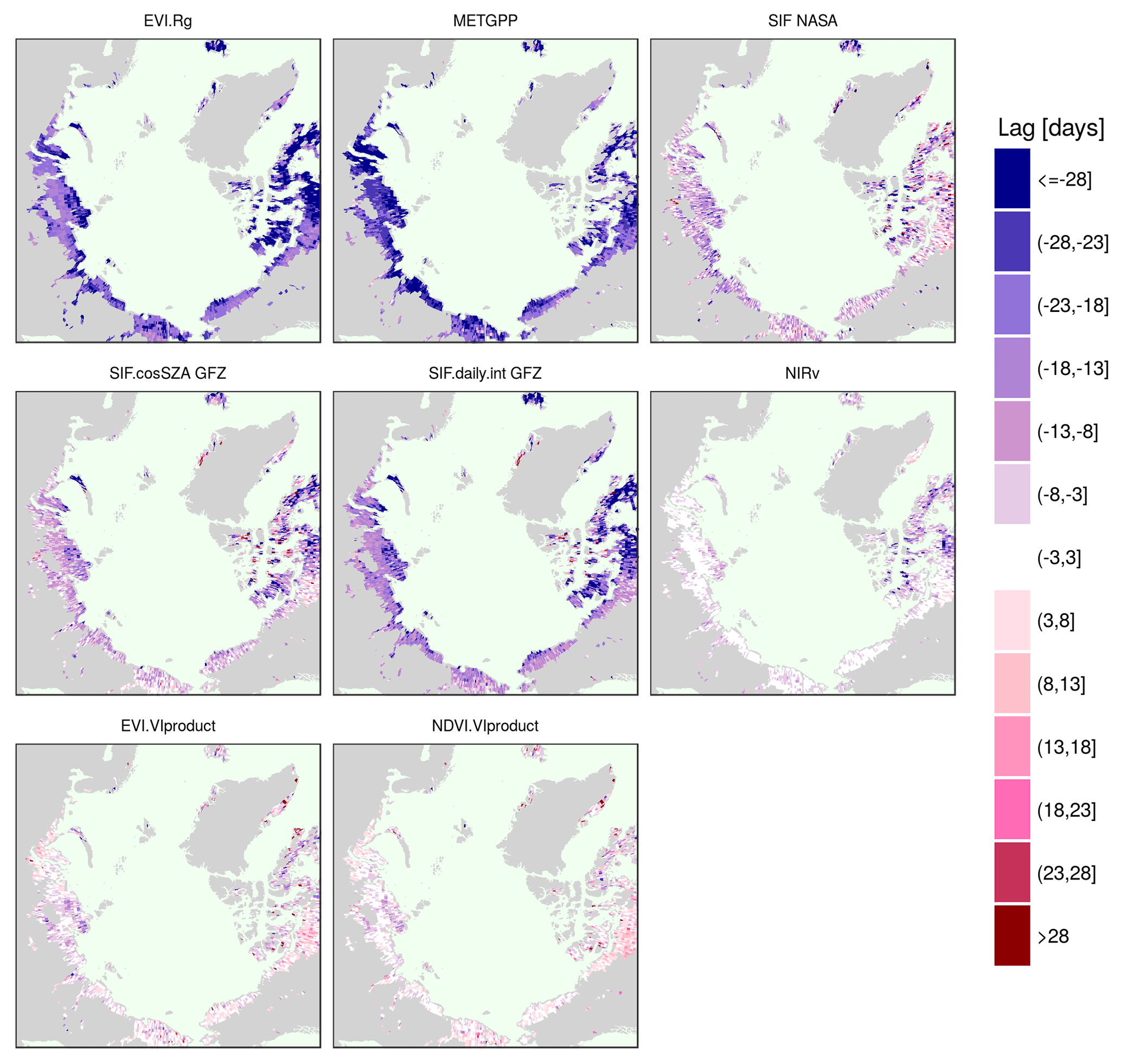
Figure A5Average time difference of the maximum across years of selected vegetation proxies and the NDVI.

Figure A6Spearman's rank correlation between the peak DOY of the vegetation proxies across years and the peak DOY of environmental variables in spatial moving windows of 1.5∘ (9 spatial pixels times 10 years at most, correlated only if more than 20 data points available). Plotted here is the variable with the highest absolute correlation without filter for statistical significance. Full correlations have been calculated (no partial correlations).
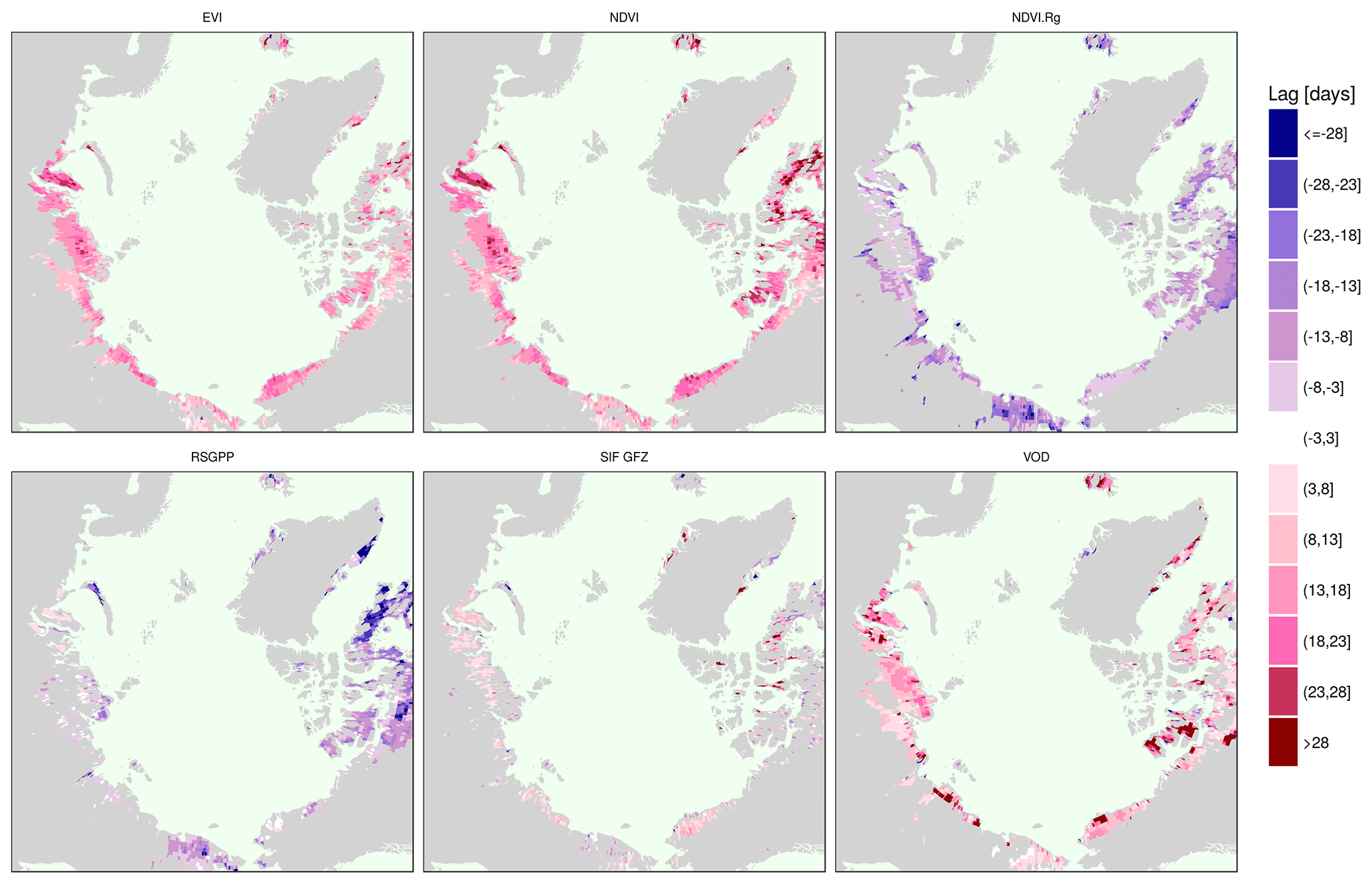
Figure A7Average time difference of the yearly maximum across years between selected vegetation proxies and the air temperature based on 50 bootstrap samples of the time series. Shown are only statistically significant differences at a level of 5 %.
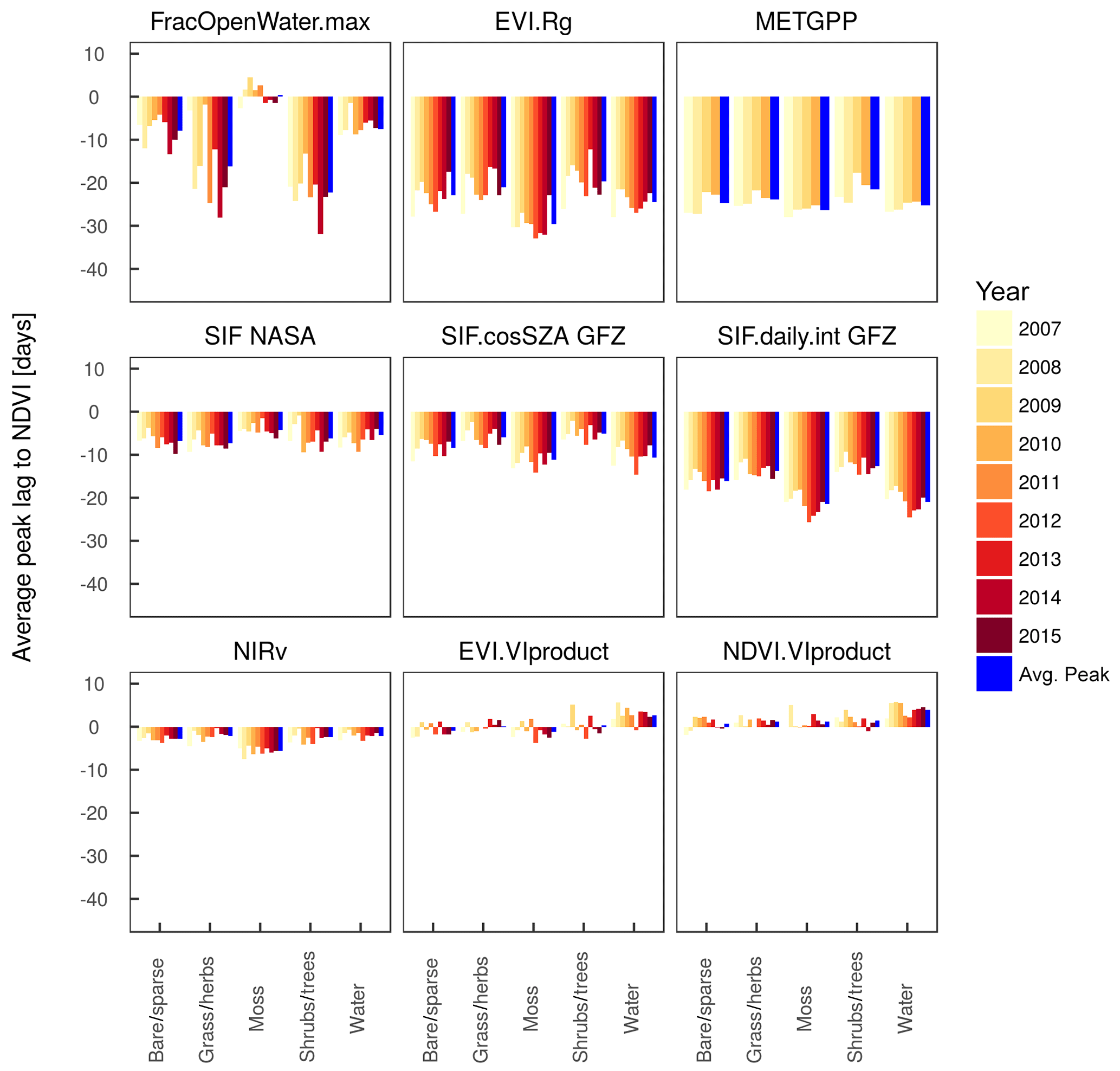
Figure A8Average of the time difference between the peaks of various variables and the NDVI as a reference per vegetation type (based on ESA CCI) and per year. The “avg.peak” represents the average of the lags in the individual years.
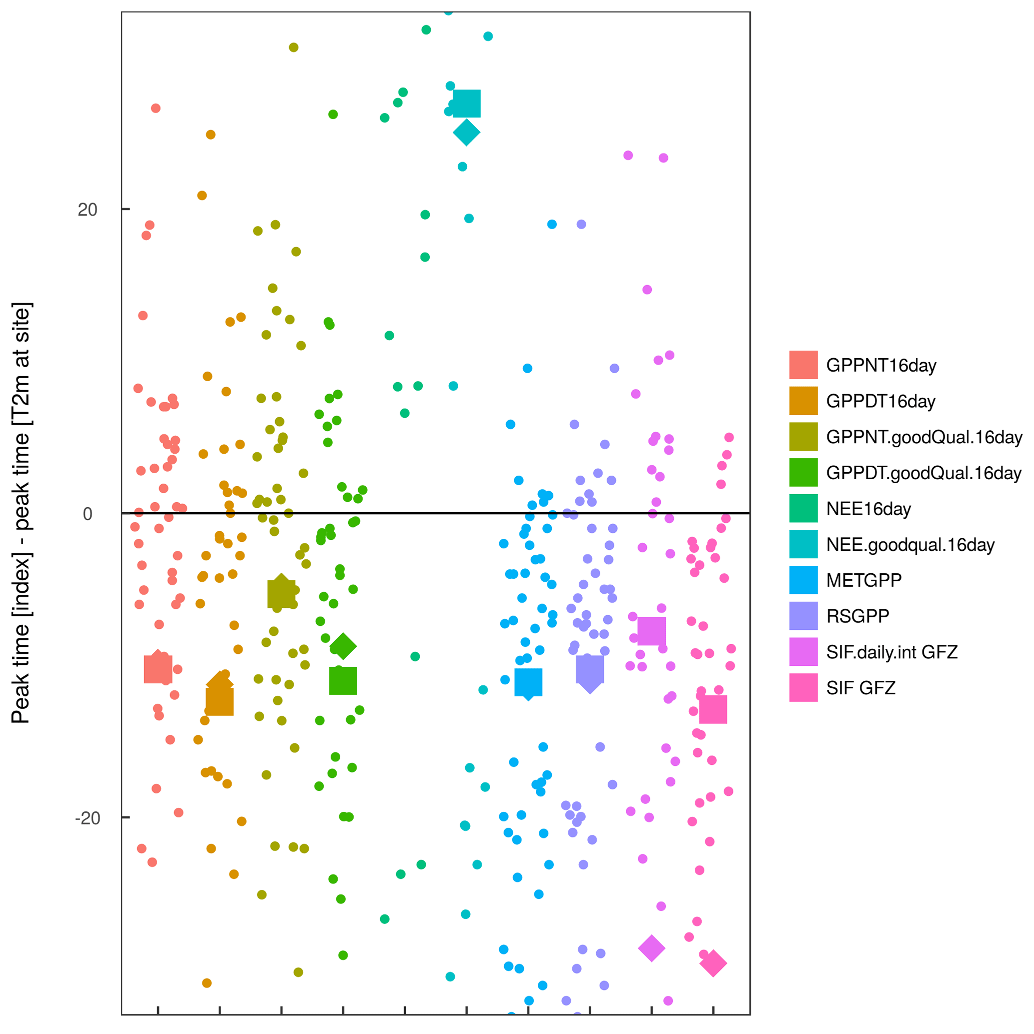
Figure A9Difference in peak timing in the different indicators to site-level temperature over years at selected FLUXNET sites. Diamonds represent the average peak lag across all years and sites, while squares indicate the average peak time across years and sites, excluding NO-Adv, DK-ZaH and DK-ZaF (where either no seasonality in SIF or strong issues between different partitioning methods are apparent).
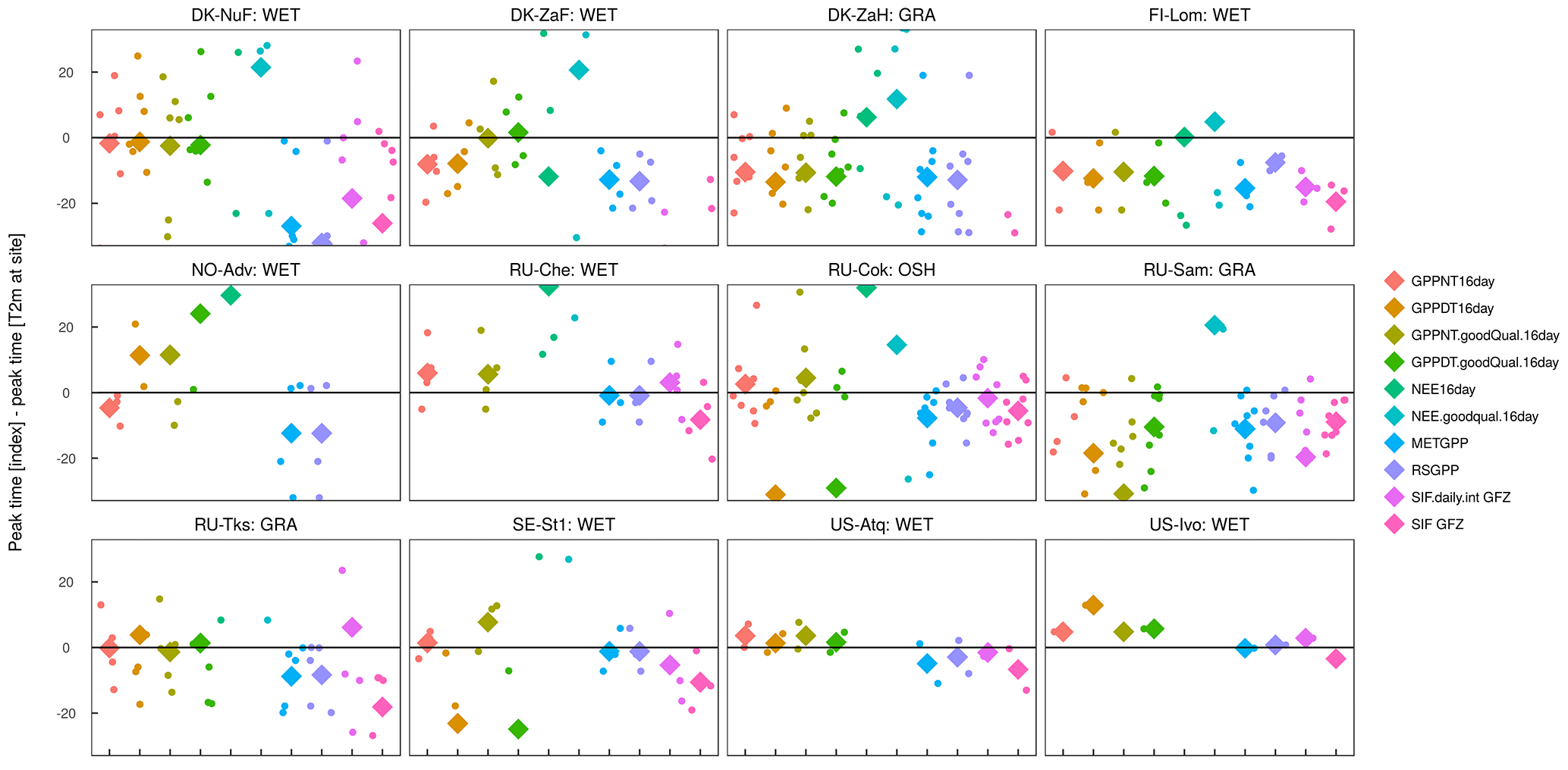
Figure A10Difference in peak timing of the different indicators to site-level temperature over years at selected FLUXNET sites. Diamonds represent the average peak lag across all years per site and variable.
Figure A11SE-St1: Time series (16 day averages) of quality filtered air temperature and NEE; blue bars indicate fraction of available good quality temperature data and gray bars indicate fraction of good and gap-filled NEE data. The middle panel depicts the GPP derived from the night-time and daytime partitioning of NEE measurements, filtered for 80 % of good quality and gap-filled NEE along with unfiltered measurements. The modelled GPP is taken from the 0.5∘ grid cell with centre coordinates closest to the tower. The bottom panel displays the 16 day averages of SIF GFZ footprints within 30 km of the site.

Figure A12DK-ZaH: Time series (16 day averages) of quality filtered air temperature and NEE; blue bars indicate fraction of available good quality temperature data and gray bars indicate fraction of good and gap-filled NEE data. The middle panel depicts the GPP derived from the night-time and daytime partitioning of NEE measurements, filtered for 80 % of good quality and gap-filled NEE along with unfiltered measurements. The modelled GPP is taken from the 0.5∘ grid cell with centre coordinates closest to the tower. The bottom panel displays the 16 day averages of SIF GFZ footprints within 30 km of the site.
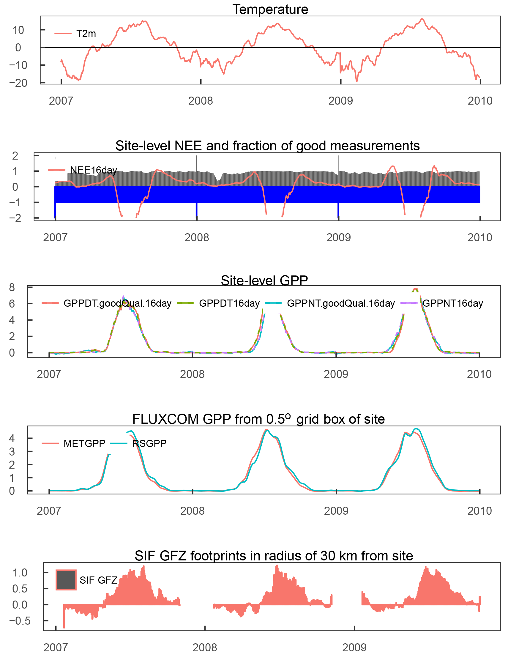
Figure A13FI-Lom: Time series (16 day averages) of quality filtered air temperature and NEE; blue bars indicate fraction of available good quality temperature data and gray bars indicate fraction of good and gap-filled NEE data. The middle panel depicts the GPP derived from the night-time and daytime partitioning of NEE measurements, filtered for 80 % of good quality and gap-filled NEE along with unfiltered measurements. The modelled GPP is taken from the 0.5∘ grid cell with centre coordinates closest to the tower. The bottom panel displays the 16 day averages of SIF GFZ footprints within 30 km of the site.
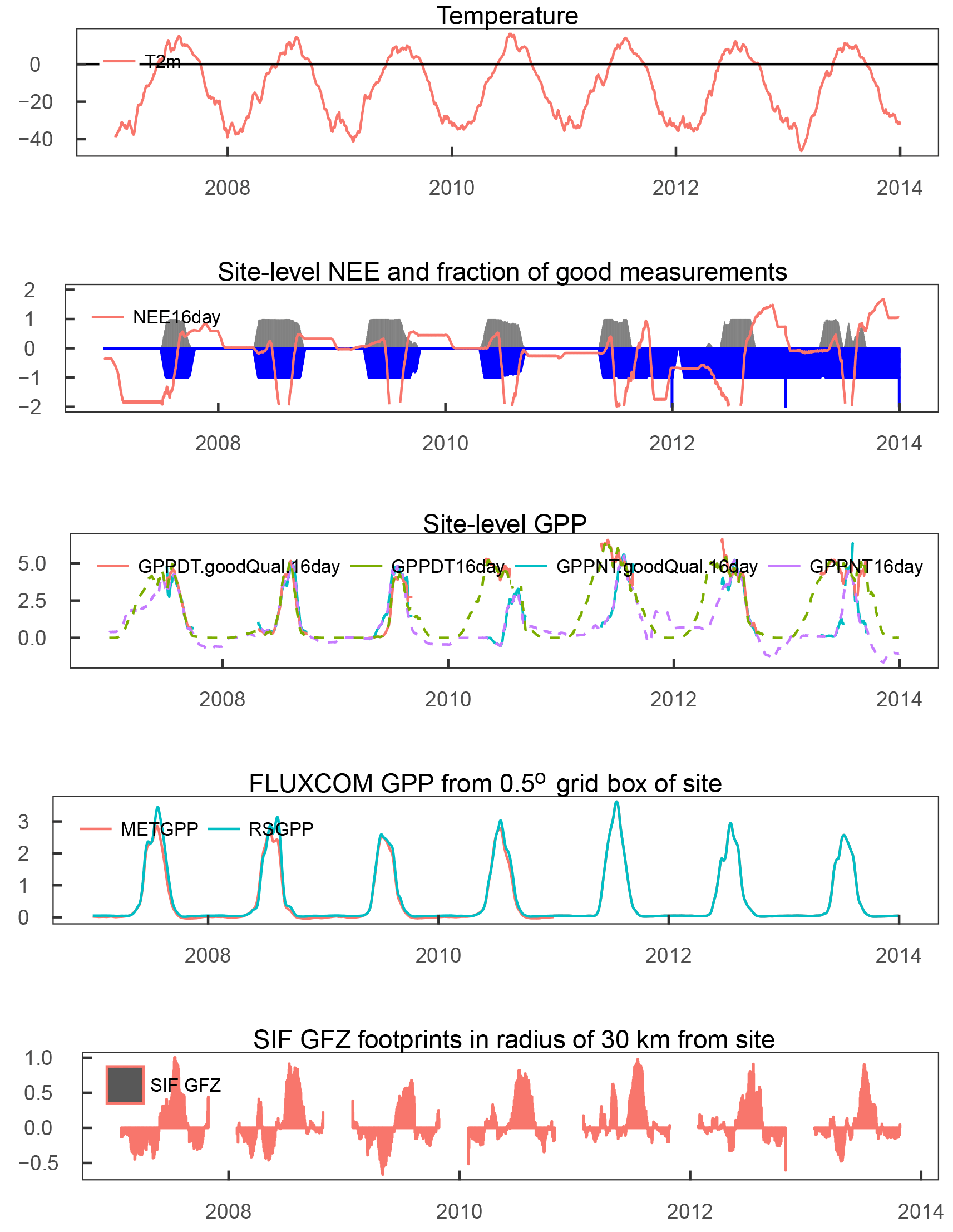
Figure A14RU-Cok: Time series (16 day averages) of quality filtered air temperature and NEE; blue bars indicate fraction of available good quality temperature data and gray bars indicate fraction of good and gap-filled NEE data. The middle panel depicts the GPP derived from the night-time and daytime partitioning of NEE measurements, filtered for 80 % of good quality and gap-filled NEE along with unfiltered measurements. The modelled GPP is taken from the 0.5∘ grid cell with centre coordinates closest to the tower. The bottom panel displays the 16 day averages of SIF GFZ footprints within 30 km of the site.
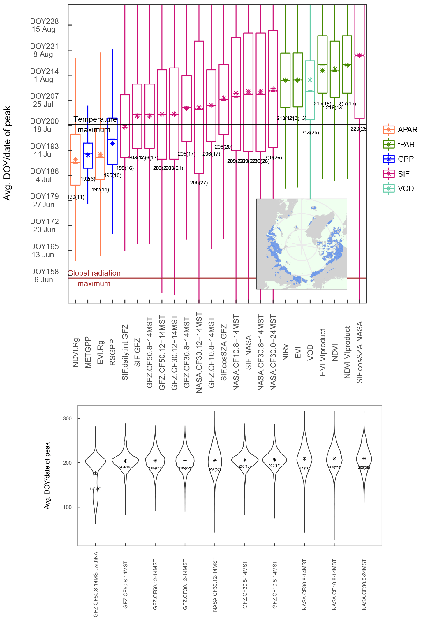
Figure A15Distribution of the annual peak DOY across years and the study area of SIF GFZ and SIF NASA, with different filters for cloud cover and over-pass time applied. Please note that the sampling of peak values is matched for each year between data sets, which explains slightly differing means and sd values depending on which vegetation proxies are included in the comparison.
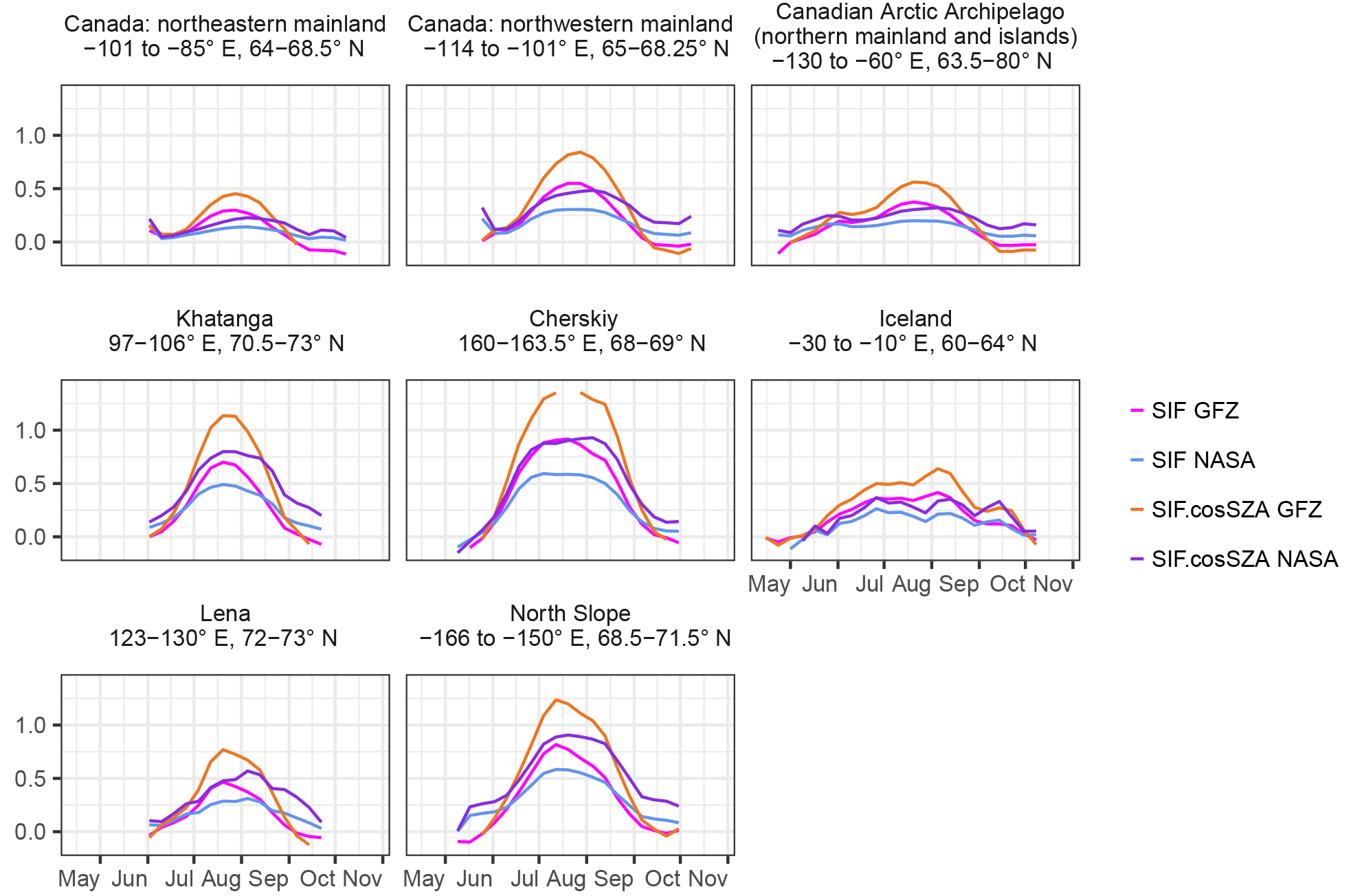
Figure A16Mean seasonal cycles of SIF data from GOME-2 for the two retrievals GFZ and NASA. Values are given in mW/(m2 sr nm).
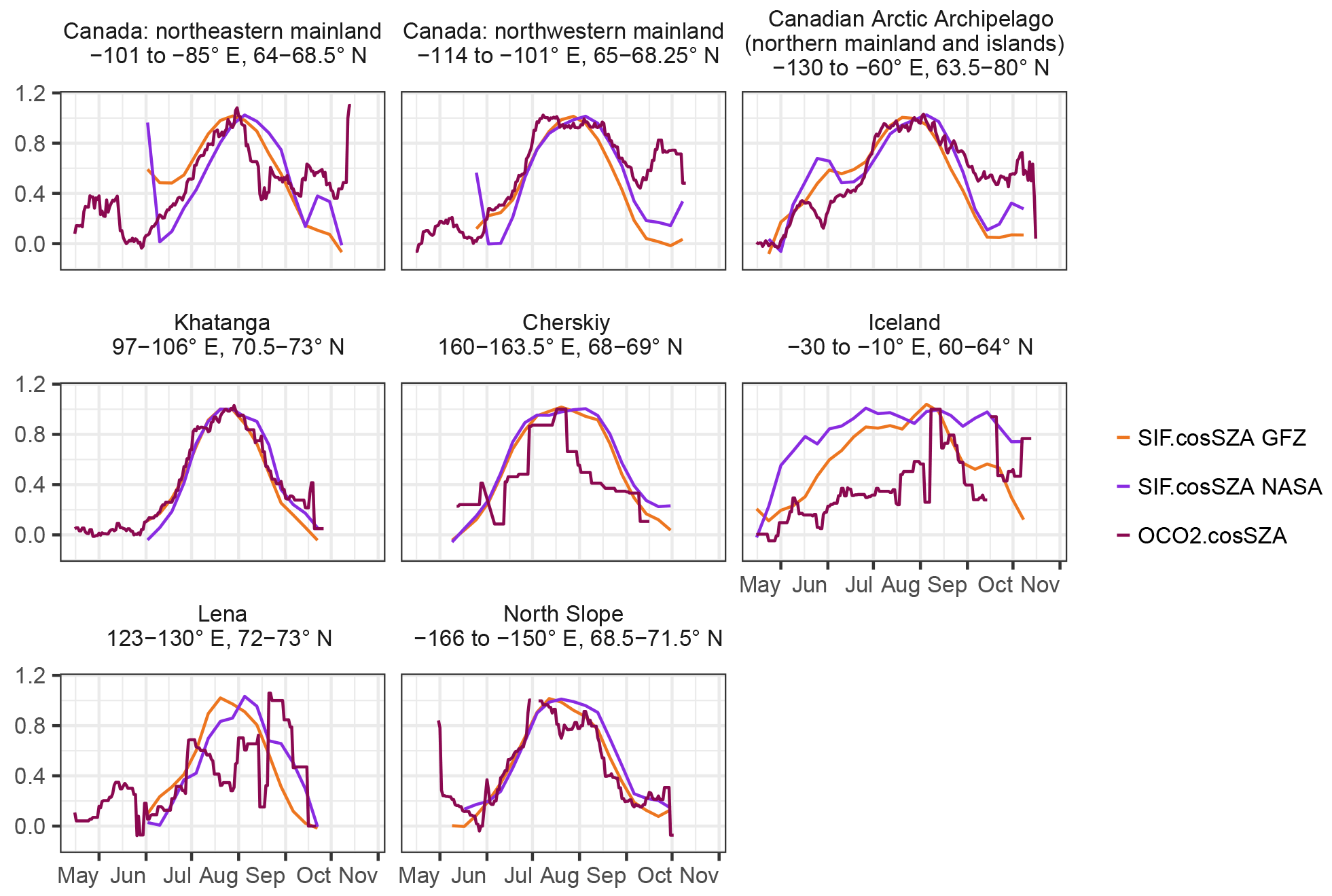
Figure A17Mean seasonal cycles of SIF data from GOME-2 and OCO-2 as a comparison. Values are scaled to 0∕1.
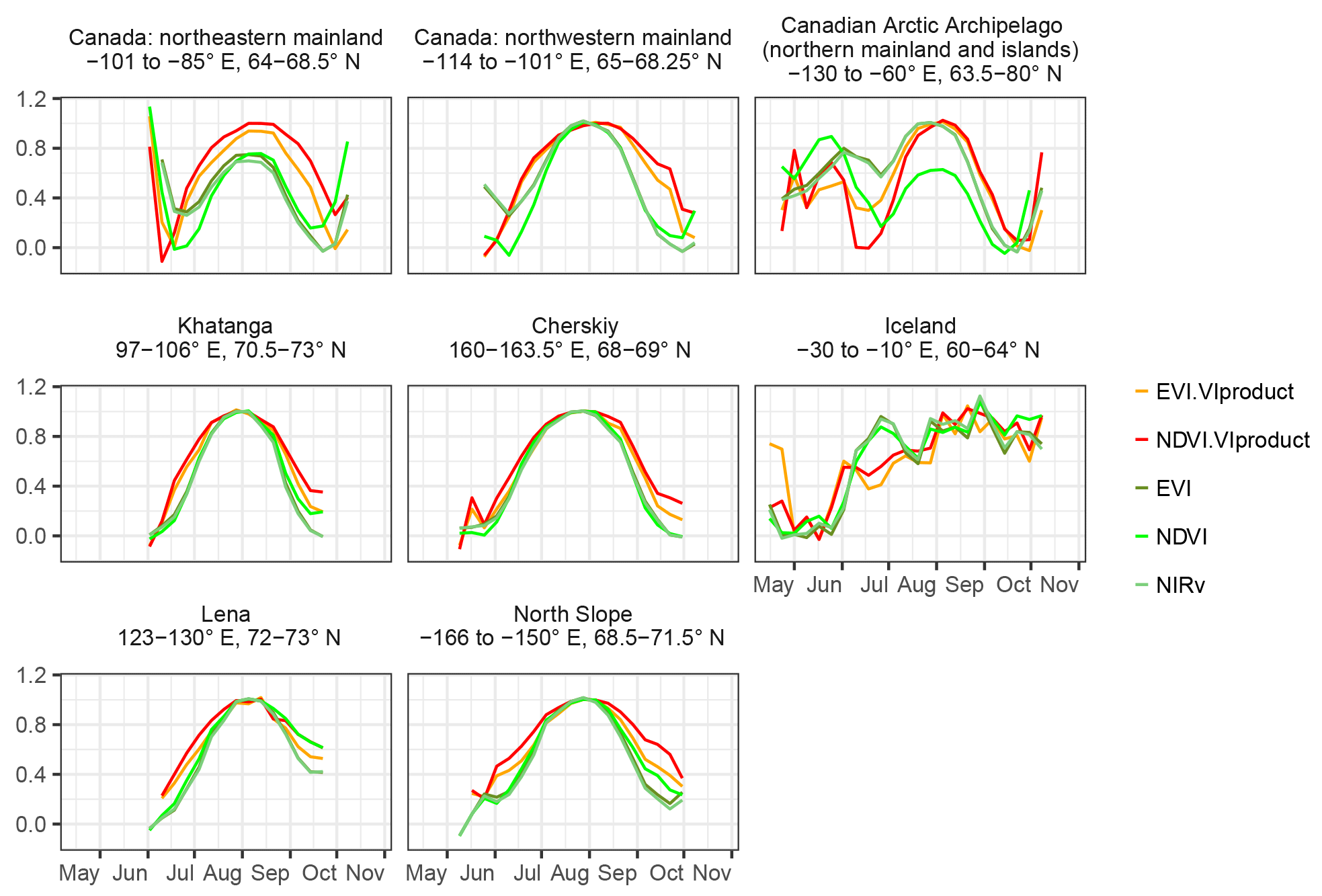
Figure A18Mean seasonal cycles of MODIS vegetation indices calculated from NBAR reflectances (MCD43C4) and as provided by the MODIS VIproduct (MxD13C1). Values are scaled to 0∕1.
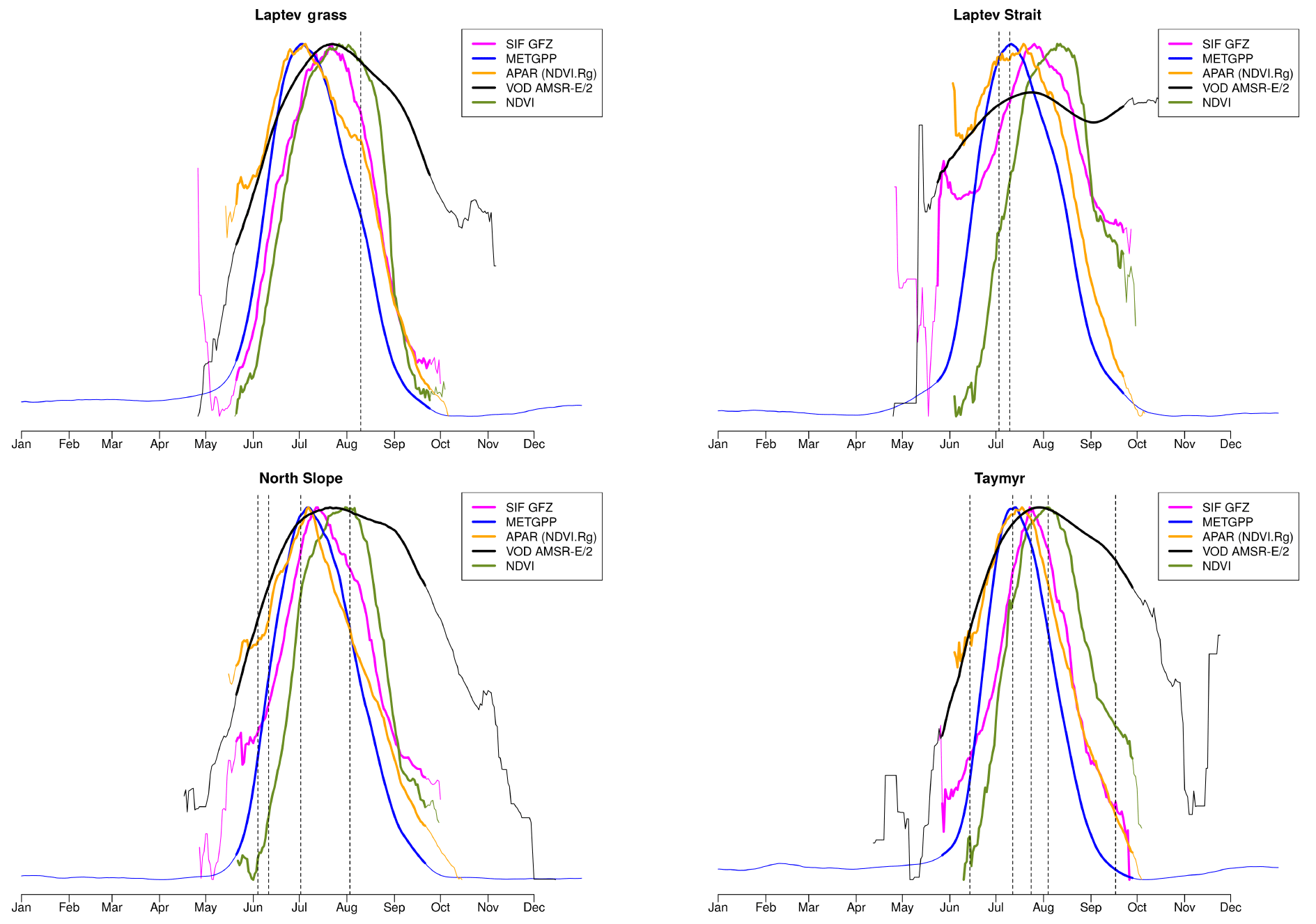
Figure A19Mean seasonal cycles of selected proxies averaged over smaller regions, as indicated in Fig. 1.
Table A1Sites and years used for a comparison of eddy-covariance derived GPP, SIF footprints within 30 km radius of the tower as well as the modelled GPP from the closest 0.5∘ grid cell.
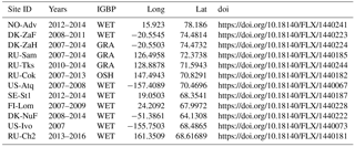
SW, LG and BH designed the research with contributions from MJ and TS. SW conducted the processing and analysis, AW processed S2 images, GD processed ESA CCI land cover data. All authors contributed to the interpretation of the results with strongest contributions from SW, LG and BH. SW wrote the manuscript with contributions from all authors.
The authors declare that they have no conflict of interest.
We thank Guido Ceccherini and Fabio Cresto-Aleina for help with polar-stereographic plotting as well as Alessandro Cescatti, Mirco Migliavacca and John Gamon for the discussion, Ulrich Weber for the processing of GlobeLand30 data and FLUXCOM data, and Ramdane Alkama for processing the Hansen forest cover data.
This work used eddy-covariance data acquired and shared by the FLUXNET community, including these networks: AmeriFlux, AfriFlux, AsiaFlux, CarboAfrica, CarboEuropeIP, CarboItaly, CarboMont, ChinaFlux, Fluxnet-Canada, GreenGrass, ICOS, KoFlux, LBA, NECC, OzFlux-TERN, TCOS-Siberia and USCCC. The ERA-Interim reanalysis data are provided by ECMWF and processed by LSCE. The FLUXNET eddy-covariance data processing and harmonization was carried out by the European Fluxes Database Cluster, AmeriFlux Management Project and Fluxdata project of FLUXNET, with the support of the CDIAC and ICOS Ecosystem Thematic Center, and the OzFlux, ChinaFlux and AsiaFlux offices.
We appreciate the permission for the use of the eddy-covariance-derived GPP and in
situ temperature measurements for the site RU-Ch2, which have been provided by
Mathias Göckede, Max-Planck-Institute for Biogeochemistry, Jena, Germany.
The article processing charges for this
open-access
publication were covered by a research
centre of the Helmholtz Association.
Edited by: David Bowling
Reviewed by: two
anonymous referees
AMAP: Arctic Climate Issues 2011: Changes in Arctic Snow, Water, Ice and Permafrost, SWIPA 2011 Overview Report, Arctic Monitoring and Assessment Programme (AMAP), Oslo, 2012. a
Arneth, A., Lloyd, J., Shibistova, O., Sogachev, A., and Kolle, O.: Spring in the boreal environment: observations on pre- and post-melt energy and CO2 fluxes in two central Siberian ecosystems, Boreal Environ. Res., 1, 311–328, 2006. a, b, c
Badgley, G., Field, C. B., and Berry, J. A.: Canopy near-infrared reflectance and terrestrial photosynthesis, Science Advances, 3, e1602244, https://doi.org/10.1126/sciadv.1602244, 2017. a
Billings, W., Luken, J., Mortensen, D., and Peterson, K.: Arctic Tundra: A Source or Sink for Atmospheric Carbon Dioxide in a Changing Environment?, Oecologia, 5, 5–1, 1982. a
Billings, W. D.: Carbon balance of Alaskan tundra and taiga ecosystems: past, present and future, Quaternary Sci. Rev., 6, 165–177, https://doi.org/10.1016/0277-3791(87)90032-1, 1987. a
Buchhorn, M., Walker, D. A., Heim, B., Raynolds, M. K., Epstein, H. E., and Schwieder, M.: Ground-Based Hyperspectral Characterization of Alaska Tundra Vegetation along Environmental Gradients, Remote Sensing, 5, 3971–4005, https://doi.org/10.3390/rs5083971, 2013. a
Cahoon, S. M. P., Sullivan, P. F., Shaver, G. R., Welker, J. M., and Post, E.: Interactions among shrub cover and the soil microclimate may determine future Arctic carbon budgets, Ecol. Lett., 15, 1415–1422, https://doi.org/10.1111/j.1461-0248.2012.01865.x, 2012. a
Cassidy, A. E., Christen, A., and Henry, G. H. R.: The effect of a permafrost disturbance on growing-season carbon-dioxide fluxes in a high Arctic tundra ecosystem, Biogeosciences, 13, 2291–2303, https://doi.org/10.5194/bg-13-2291-2016, 2016. a
Chadburn, S. E., Krinner, G., Porada, P., Bartsch, A., Beer, C., Belelli Marchesini, L., Boike, J., Ekici, A., Elberling, B., Friborg, T., Hugelius, G., Johansson, M., Kuhry, P., Kutzbach, L., Langer, M., Lund, M., Parmentier, F.-J. W., Peng, S., Van Huissteden, K., Wang, T., Westermann, S., Zhu, D., and Burke, E. J.: Carbon stocks and fluxes in the high latitudes: using site-level data to evaluate Earth system models, Biogeosciences, 14, 5143–5169, https://doi.org/10.5194/bg-14-5143-2017, 2017. a, b
Chapin, F. S., Shaver, G., Giblin, A., Nadelhoffer, K., and Laundre, J.: Responses of Arctic Tundra to Experimental and Observed Changes in Climate, Ecology, 76, 694–711, https://doi.org/10.2307/1939337, 1995. a, b
Chapin, F. S. I.: Environmental controls over growth of tundra plants, Ecol. Bull., 38, 69–76, 1987. a, b, c
Chen, J., Chen, J., Liao, A., Cao, X., Chen, L., Chen, X., He, C., Han, G., Peng, S., Lu, M., Zhang, W., Tong, X., and Mills, J.: Global land cover mapping at 30 m resolution: A POK-based operational approach, ISPRS J. Photogramm., 103, 7–27, https://doi.org/10.1016/j.isprsjprs.2014.09.002, 2015. a
Commane, R., Lindaas, J., Benmergui, J., Luus, K. A., Chang, R. Y.-W., Daube, B. C., Euskirchen, E. S., Henderson, J. M., Karion, A., Miller, J. B., Miller, S. M., Parazoo, N. C., Randerson, J. T., Sweeney, C., Tans, P., Thoning, K., Veraverbeke, S., Miller, C. E., and Wofsy, S. C.: Carbon dioxide sources from Alaska driven by increasing early winter respiration from Arctic tundra, P. Natl. Acad. Sci. USA, 114, 5361–5366, https://doi.org/10.1073/pnas.1618567114, 2017. a
Dass, P., Rawlins, M. A., Kimball, J. S., and Kim, Y.: Environmental controls on the increasing GPP of terrestrial vegetation across northern Eurasia, Biogeosciences, 13, 45–62, https://doi.org/10.5194/bg-13-45-2016, 2016. a
Dee, D. P., Uppala, S. M., Simmons, A. J., Berrisford, P., Poli, P., Kobayashi, S., Andrae, U., Balmaseda, M. A., Balsamo, G., Bauer, P., Bechtold, P., Beljaars, A. C. M., van de Berg, L., Bidlot, J., Bormann, N., Delsol, C., Dragani, R., Fuentes, M., Geer, A. J., Haimberger, L., Healy, S. B., Hersbach, H., Hólm, E. V., Isaksen, L., Kållberg, P., Köhler, M., Matricardi, M., McNally, A. P., Monge-Sanz, B. M., Morcrette, J.-J., Park, B.-K., Peubey, C., de Rosnay, P., Tavolato, C., Thépaut, J.-N., and Vitart, F.: The ERA-Interim reanalysis: configuration and performance of the data assimilation system, Q. J. Roy. Meteor. Soc., 137, 553–597, https://doi.org/10.1002/qj.828, 2011. a
Doelling, D. R., Loeb, N. G., Keyes, D. F., Nordeen, M. L., Morstad, D., Nguyen, C., Wielicki, B. A., Young, D. F., and Sun, M.: Geostationary Enhanced Temporal Interpolation for CERES Flux Products, J. Atmos. Ocean. Tech., 30, 1072–1090, https://doi.org/10.1175/JTECH-D-12-00136.1, 2013. a
Du, J., Jones, L. A., and Kimball, J. S.: Daily Global Land Parameters Derived from AMSR-E and AMSR2, Version 2 [GeoTIFF 2007-2016], https://doi.org/10.5067/RF8WPYOPJKL2, 2017a. a
Du, J., Kimball, J. S., Jones, L. A., Kim, Y., Glassy, J., and Watts, J. D.: A global satellite environmental data record derived from AMSR-E and AMSR2 microwave Earth observations, Earth Syst. Sci. Data, 9, 791–808, https://doi.org/10.5194/essd-9-791-2017, 2017b. a, b
Elmendorf, S. C., Henry, G. H. R., Hollister, R. D., Björk, R. G., Boulanger-Lapointe, N., Cooper, E. J., Cornelissen, J. H. C., Day, T. A., Dorrepaal, E., Elumeeva, T. G., Gill, M., Gould, W. A., Harte, J., Hik, D. S., Hofgaard, A., Johnson, D. R., Johnstone, J. F., Jónsdóttir, I. S., Jorgenson, J. C., Klanderud, K., Klein, J. A., Koh, S., Kudo, G., Lara, M., Lévesque, E., Magnússon, B., May, J. L., Mercado-Díaz, J. A., Michelsen, A., Molau, U., Myers-Smith, I. H., Oberbauer, S. F., Onipchenko, V. G., Rixen, C., Schmidt, N. M., Shaver, G. R., Spasojevic, M. J., Þórhallsdóttir, P. E., Tolvanen, A., Troxler, T., Tweedie, C. E., Villareal, S., Wahren, C.-H., Walker, X., Webber, P. J., Welker, J. M., and Wipf, S.: Plot-scale evidence of tundra vegetation change and links to recent summer warming, Nat. Clim. Change, 2, 453–457, https://doi.org/10.1038/NCLIMATE1465, 2012. a
Emmerton, C. A., St. Louis, V. L., Humphreys, E. R., Gamon, J. A., Barker, J. D., and Pastorello, G. Z.: Net ecosystem exchange of CO2 with rapidly changing high Arctic landscapes, Glob. Change Biol., 22, 1185–1200, https://doi.org/10.1111/gcb.13064, 2016. a, b
Frankenberg, C., O'Dell, C., Guanter, L., and McDuffie, J.: Remote sensing of near-infrared chlorophyll fluorescence from space in scattering atmospheres: implications for its retrieval and interferences with atmospheric CO2 retrievals, Atmos. Meas. Tech., 5, 2081–2094, https://doi.org/10.5194/amt-5-2081-2012, 2012. a
Frankenberg, C., O'Dell, C., Berry, J., Guanter, L., Joiner, J., Köhler, P., Pollock, R., and Taylor, T. E.: Prospects for chlorophyll fluorescence remote sensing from the Orbiting Carbon Observatory-2, Remote Sens. Environ., 147, 1–12, https://doi.org/10.1016/j.rse.2014.02.007, 2014. a
Gamon, J., Huemmrich, K., Stone, R., and Tweedie, C.: Spatial and temporal variation in primary productivity (NDVI) of coastal Alaskan tundra: Decreased vegetation growth following earlier snowmelt, Remote Sens. Environ., 129, 144–153, https://doi.org/10.1016/j.rse.2012.10.030, 2013. a, b, c, d, e, f, g, h
Gamon, J. A., Penuelas, J. P., and Field, C. B.: A narrow-waveband spectral index that tracks diurnal changes in photosynthetic efficiency, Remote Sens. Environ., 41, 35–44, https://doi.org/10.1016/0034-4257(92)90059-S, 1992. a
Gamon, J. A., Huemmrich, K. F., Wong, C. Y. S., Ensminger, I., Garrity, S., Hollinger, D. Y., Noormets, A., and Peñuelas, J.: A remotely sensed pigment index reveals photosynthetic phenology in evergreen conifers, P. Natl. Acad. Sci. USA, 113, 13087–13092, https://doi.org/10.1073/pnas.1606162113, 2016. a
Grant, J. P., Wigneron, J.-P., De Jeu, R. A. M., Lawrence, H., Mialon, A., Richaume, P., Al Bitar, A., Drusch, M., van Marle, M. J. E., and Kerr, Y.: Comparison of {SMOS} and AMSR-E vegetation optical depth to four MODIS-based vegetation indices, Remote Sens. Environ., 172, 787–100, https://doi.org/10.1016/j.rse.2015.10.021, 2016. a
Hansen, M. C., Potapov, P. V., Moore, R., Hancher, M., Turubanova, S. A., Tyukavina, A., Thau, D., Stehman, S. V., Goetz, S. J., Loveland, T. R., Kommareddy, A., Egorov, A., Chini, L., Justice, C. O., and Townshend, J. R. G.: High-Resolution Global Maps of 21st-Century Forest Cover Change, Science, 342, 850–853, https://doi.org/10.1126/science.1244693, 2013. a, b, c, d
Huemmrich, K. F., Gamon, J., Tweedie, C., Oberbauer, S., Kinoshita, G., Houston, S., Kuchy, A., Hollister, R., Kwon, H., Mano, M., Harazono, Y., Webber, P., and Oechel, W.: Remote sensing of tundra gross ecosystem productivity and light use efficiency under varying temperature and moisture conditions, Remote Sens. Environ., 114, 481–489, https://doi.org/10.1016/j.rse.2009.10.003, 2010a. a, b, c, d
Huemmrich, K. F., Kinoshita, G., Gamon, J. A., Houston, S., Kwon, H., and Oechel, W. C.: Tundra carbon balance under varying temperature and moisture regimes, J. Geophys. Res., 11, g00I025, https://doi.org/10.1029/2009JG001237, 2010b. a, b, c, d
Huemmrich, K. F., Gamon, J., Tweedie, C., Campbell, P., Landis, D., and Middleton, E.: Arctic Tundra Vegetation Functional Types Based on Photosynthetic Physiology and Optical Properties, IEEE J. Sel. Top. Appl., 6, 265–275, https://doi.org/10.1109/JSTARS.2013.2253446, 2013. a, b
Huete, A., Didan, K., Miura, T., Rodriguez, E., Gao, X., and Ferreira, L.: Overview of the radiometric and biophysical performance of the MODIS vegetation indices, Remote Sens. Environ., 83, 195–213, 2002. a
Jia, G. J., Epstein, H. E., and Walker, D. A.: Greening of arctic Alaska, 1981–2001, Geophys. Res. Lett., 30, 2067, https://doi.org/10.1029/2003GL018268, 2003. a
Joiner, J., Yoshida, Y., Vasilkov, A. P., Middleton, E. M., Campbell, P. K. E., Yoshida, Y., Kuze, A., and Corp, L. A.: Filling-in of near-infrared solar lines by terrestrial fluorescence and other geophysical effects: simulations and space-based observations from SCIAMACHY and GOSAT, Atmos. Meas. Tech., 5, 809–829, https://doi.org/10.5194/amt-5-809-2012, 2012. a
Joiner, J., Guanter, L., Lindstrot, R., Voigt, M., Vasilkov, A. P., Middleton, E. M., Huemmrich, K. F., Yoshida, Y., and Frankenberg, C.: Global monitoring of terrestrial chlorophyll fluorescence from moderate-spectral-resolution near-infrared satellite measurements: methodology, simulations, and application to GOME-2, Atmos. Meas. Tech., 6, 2803–2823, https://doi.org/10.5194/amt-6-2803-2013, 2013. a
Joiner, J., Yoshida, Y., Guanter, L., and Middleton, E. M.: New methods for the retrieval of chlorophyll red fluorescence from hyperspectral satellite instruments: simulations and application to GOME-2 and SCIAMACHY, Atmos. Meas. Tech., 9, 3939–3967, https://doi.org/10.5194/amt-9-3939-2016, 2016. a
Jones, M. O., Jones, L. A., Kimball, J. S., and McDonald, K. C.: Satellite passive microwave remote sensing for monitoring global land surface phenology, Remote Sens. Environ., 115, 1102–1114, https://doi.org/10.1016/j.rse.2010.12.015, 2011. a
Kobayashi, H., Yunus, A. P., Nagai, S., Sugiura, K., Kim, Y., Van Dam, B., Nagano, H., Zona, D., Harazono, Y., Bret-Harte, M. S., Ichii, K., Ikawa, H., Iwata, H., Oechel, W. C., Ueyama, M., and Suzuki, R.: Latitudinal gradient of spruce forest understory and tundra phenology in Alaska as observed from satellite and ground-based data, Remote Sens. Environ., 177, 160–170, https://doi.org/10.1016/j.rse.2016.02.020, 2016. a
Köhler, P., Guanter, L., and Joiner, J.: A linear method for the retrieval of sun-induced chlorophyll fluorescence from GOME-2 and SCIAMACHY data, Atmos. Meas. Tech., 8, 2589–2608, https://doi.org/10.5194/amt-8-2589-2015, 2015. a, b
Kross, A. S. E., Roulet, N. T., Moore, T. R., Lafleur, P. M., Humphreys, E. R., Seaquist, J. W., Flanagan, L. B., and Aurela, M.: Phenology and its role in carbon dioxide exchange processes in northern peatlands, J. Geophys. Res.-Biogeo., 119, 1370–1384, https://doi.org/10.1002/2014JG002666, 2014. a, b, c
Kwon, H.-J., Oechel, W. C., Zulueta, R. C., and Hastings, S.: Effects of climate variability on carbon sequestration among adjacent wet sedge tundra and moist tussock tundra ecosystems, J. Geophys. Res.-Biogeo., 111, g03014, https://doi.org/10.1029/2005JG000036, 2006. a
Lafleur, P. M. and Humphreys, E. R.: Spring warming and carbon dioxide exchange over low Arctic tundra in central Canada, Glob. Change Biol., 14, 740–756, https://doi.org/10.1111/j.1365-2486.2007.01529.x, 2008. a, b, c, d
Laidler, G. J. and Treitz, P.: Biophysical remote sensing of arctic environments, Prog. Phys. Geogr., 27, 44–68, https://doi.org/10.1191/0309133303pp358ra, 2003. a
Liu, Y. Y., de Jeu, R. A. M., McCabe, M. F., Evans, J. P., and van Dijk, A. I. J. M.: Global long-term passive microwave satellite-based retrievals of vegetation optical depth, Geophys. Res. Lett., 38, l18402, https://doi.org/10.1029/2011GL048684, 2011. a, b, c
López-Blanco, E., Lund, M., Williams, M., Tamstorf, M. P., Westergaard-Nielsen, A., Exbrayat, J.-F., Hansen, B. U., and Christensen, T. R.: Exchange of CO2 in Arctic tundra: impacts of meteorological variations and biological disturbance, Biogeosciences, 14, 4467–4483, https://doi.org/10.5194/bg-14-4467-2017, 2017. a, b
Lund, M., Lafleur, P. M., Roulet, N. T., Lindroth, A., Christensen, T. R., Aurela, M., Chojnicki, B. H., Flanagan, L. B., Humphreys, E. R., Laurila, T., Oechel, W. C., Olejnik, J., Rinne, J., Schubert, P., and Nilsson, M. B.: Variability in exchange of CO2 across 12 northern peatland and tundra sites, Glob. Change Biol., 16, 2436–2448, https://doi.org/10.1111/j.1365-2486.2009.02104.x, 2010. a, b
Luus, K. A., Commane, R., Parazoo, N. C., Benmergui, J., Euskirchen, E. S., Frankenberg, C., Joiner, J., Lindaas, J., Miller, C. E., Oechel, W. C., Zona, D., Wofsy, S., and Lin, J. C.: Tundra photosynthesis captured by satellite-observed solar-induced chlorophyll fluorescence, Geophys. Res. Lett., 44, 1564–1573, https://doi.org/10.1002/2016GL070842, 2017. a, b, c
Martens, B., Miralles, D. G., Lievens, H., van der Schalie, R., de Jeu, R. A. M., Fernández-Prieto, D., Beck, H. E., Dorigo, W. A., and Verhoest, N. E. C.: GLEAM v3: satellite-based land evaporation and root-zone soil moisture, Geosci. Model Dev., 10, 1903–1925, https://doi.org/10.5194/gmd-10-1903-2017, 2017. a
Marushchak, M. E., Kiepe, I., Biasi, C., Elsakov, V., Friborg, T., Johansson, T., Soegaard, H., Virtanen, T., and Martikainen, P. J.: Carbon dioxide balance of subarctic tundra from plot to regional scales, Biogeosciences, 10, 437–452, https://doi.org/10.5194/bg-10-437-2013, 2013. a, b, c
May, J. L., Healey, N. C., Ahrends, H. E., Hollister, R. D., Tweedie, C. E., Welker, J. M., Gould, W. A., and Oberbauer, S. F.: Short-Term Impacts of the Air Temperature on Greening and Senescence in Alaskan Arctic Plant Tundra Habitats, Remote Sensing, 9, 1338, https://doi.org/10.3390/rs9121338, 2017. a, b
MCD43C4 (NASA LP DAAC, U. E. R. O. and Science (EROS) Center, Sioux Falls, South Dakota): MCD43C4: MODIS/Terra and Aqua Nadir BRDF-Adjusted Reflectance Daily L3 Global 0.05Deg CMG V006, https://doi.org/10.5067/MODIS/MCD43C4.006, 2017. a
McFadden, J. P., Eugster, W., and Chapin, F. S.: A REGIONAL STUDY OF THE CONTROLS ON WATER VAPOR AND CO2 EXCHANGE IN ARCTIC TUNDRA, Ecology, 84, 2762–2776, https://doi.org/10.1890/01-0444, 2003. a, b, c
McGuire, A. D., Christensen, T. R., Hayes, D., Heroult, A., Euskirchen, E., Kimball, J. S., Koven, C., Lafleur, P., Miller, P. A., Oechel, W., Peylin, P., Williams, M., and Yi, Y.: An assessment of the carbon balance of Arctic tundra: comparisons among observations, process models, and atmospheric inversions, Biogeosciences, 9, 3185–3204, https://doi.org/10.5194/bg-9-3185-2012, 2012. a, b
Miralles, D. G., Holmes, T. R. H., De Jeu, R. A. M., Gash, J. H., Meesters, A. G. C. A., and Dolman, A. J.: Global land-surface evaporation estimated from satellite-based observations, Hydrol. Earth Syst. Sci., 15, 453–469, https://doi.org/10.5194/hess-15-453-2011, 2011. a
MOD13C1 (NASA LP DAAC, U. E. R. O. and Science (EROS) Center, Sioux Falls, South Dakota): MOD13C1: MODIS/Terra Vegetation Indices 16-Day L3 Global 0.05 Deg CMG V006, https://doi.org/10.5067/MODIS/MOD13C1.006, 2017. a
Monteith, J. L.: Solar Radiation and Productivity in Tropical Ecosystems, J. Appl. Ecol., 9, 747–766, 1972. a, b
MYD13C1 (NASA LP DAAC, U. E. R. O. and Science (EROS) Center, Sioux Falls, S. D.): MYD13C1: MODIS/Aqua Vegetation Indices 16-Day L3 Global 0.05 Deg CMG V006, https://doi.org/10.5067/MODIS/MYD13C1.006, 2017. a
Myneni, R. B., Keeling, C. D., Tucker, C. J., Asrar, G., and Nemani, R. R.: Increased plant growth in the northern high latitudes from 1981 to 1991, Nature, 386, 698–702, https://doi.org/10.1038/386698a0, 1997. a
Oberbauer, S. F., Starr, G., and Pop, E. W.: Effects of extended growing season and soil warming on carbon dioxide and methane exchange of tussock tundra in Alaska, J. Geophys. Res., 103, 29075–29082, 1998. a
OCO-2 Science Team/Michael Gunson, A. E.: OCO2 L2 Lite SIF; OCO-2 Level 2 bias-corrected solar-induced fluorescence and other select fields from the IMAP-DOAS algorithm aggregated as daily files, version 8, NASA Goddard Earth Science Data and Information Services Center (GES DISC), Greenbelt, MD, USA, 2017. a
Oechel, W. C., Hastings, S. J., Vourlrtis, G., Jenkins, M., Riechers, G., and Grulke, N.: Recent change of Arctic tundra ecosystems from a net carbon dioxide sink to a source, Nature, 361, 520–523, https://doi.org/10.1038/361520a0, 1993. a, b
Olivas, P. C., Oberbauer, S. F., Tweedie, C., Oechel, W. C., Lin, D., and Kuchy, A.: Effects of Fine-Scale Topography on CO2 Flux Components of Alaskan Coastal Plain Tundra: Response to Contrasting Growing Seasons, Arct. Antarct. Alp. Res., 43, 256–266, https://doi.org/10.1657/1938-4246-43.2.256, 2011. a, b, c, d, e
Opała-Owczarek, M., Pirożnikow, E., Owczarek, P., Szymański, W., Luks, B., Kȩpski, D., Szymanowski, M., Wojtuń, B., and Migała, K.: The influence of abiotic factors on the growth of two vascular plant species (Saxifraga oppositifolia and Salix polaris) in the High Arctic, Catena, 163, 219–232, https://doi.org/10.1016/j.catena.2017.12.018, 2018. a
Parazoo, N. C., Arneth, A., Pugh, T. A. M., Smith, B., Steiner, N., Luus, K., Commane, R., Benmergui, J., Stofferahn, E., Liu, J., Rödenbeck, C., Kawa, R., Euskirchen, E., Zona, D., Arndt, K., Oechel, W., and Miller, C.: Spring photosynthetic onset and net CO2 uptake in Alaska triggered by landscape thawing, Glob. Change Biol., 24, 3416–3435, https://doi.org/10.1111/gcb.14283, 2018. a, b, c, d, e
Parida, B. R. and Buermann, W.: Increasing summer drying in North American ecosystems in response to longer nonfrozen periods, Geophys. Res. Lett., 41, 5476–5483, https://doi.org/10.1002/2014GL060495, 2014. a
Pearson, R. G., Phillips, S. J., Loranty, M. M., Beck, P. S. A., Damoulas, T., Knight, S. J., and Goetz, S. J.: Shifts in Arctic vegetation and associated feedbacks under climate change, Nat. Clim. Change, 3, 673–677, https://doi.org/10.1038/nclimate1858, 2013. a
Pirk, N., Sievers, J., Mertes, J., Parmentier, F.-J. W., Mastepanov, M., and Christensen, T. R.: Spatial variability of CO2 uptake in polygonal tundra: assessing low-frequency disturbances in eddy covariance flux estimates, Biogeosciences, 14, 3157–3169, https://doi.org/10.5194/bg-14-3157-2017, 2017. a, b, c, d, e, f
Porcar-Castell, A., Tyystjärvi, E., Atherton, J., van der Tol, C., Flexas, J., Pfündel, E. E., Moreno, J., Frankenberg, C., and Berry, J. A.: Linking chlorophyll a fluorescence to photosynthesis for remote sensing applications: mechanisms and challenges, J. Exp. Bot., 65, 4065–4095, https://doi.org/10.1093/jxb/eru191, 2014. a, b
Poulter, B., MacBean, N., Hartley, A., Khlystova, I., Arino, O., Betts, R., Bontemps, S., Boettcher, M., Brockmann, C., Defourny, P., Hagemann, S., Herold, M., Kirches, G., Lamarche, C., Lederer, D., Ottlé, C., Peters, M., and Peylin, P.: Plant functional type classification for earth system models: results from the European Space Agency's Land Cover Climate Change Initiative, Geosci. Model Dev., 8, 2315–2328, https://doi.org/10.5194/gmd-8-2315-2015, 2015. a
Reichstein, M., Falge, E., Baldocchi, D., Papale, D., Aubinet, M., Berbigier, P., Bernhofer, C., Buchmann, N., Gilmanov, T., Granier, A., Grünwald, T., Havránková, K., Ilvesniemi, H., Janous, D., Knohl, A., Laurila, T., Lohila, A., Loustau, D., Matteucci, G., Meyers, T., Miglietta, F., Ourcival, J.-M., Pumpanen, J., Rambal, S., Rotenberg, E., Sanz, M., Tenhunen, J., Seufert, G., Vaccari, F., Vesala, T., Yakir, D., and Valentini, R.: On the separation of net ecosystem exchange into assimilation and ecosystem respiration: review and improved algorithm, Glob. Change Biol., 11, 1424–1439, https://doi.org/10.1111/j.1365-2486.2005.001002.x, 2005. a
Riedel, S. M., Epstein, H. E., and Walker, D. A.: Biotic controls over spectral reflectance of arctic tundra vegetation, Int. J. Remote Sens., 26, 2391–2405, https://doi.org/10.1080/01431160512331337754, 2005. a
Rogers, A., Serbin, S., Ely, K., Sloan, V., and Wullschleger, S.: Terrestrial biosphere models underestimate photosynthetic capacity and CO2 assimilation in the Arctic, New Phytol., 216, 1090–1103, https://doi.org/10.1111/nph.14740, 2017. a, b
Runkle, B. R. K., Sachs, T., Wille, C., Pfeiffer, E.-M., and Kutzbach, L.: Bulk partitioning the growing season net ecosystem exchange of CO2 in Siberian tundra reveals the seasonality of its carbon sequestration strength, Biogeosciences, 10, 1337–1349, https://doi.org/10.5194/bg-10-1337-2013, 2013. a, b
Sitch, S., McGuire, A. D., Kimball, J., Gedney, N., Gamon, J., Engstrom, R., Wolf, A., Zhuang, Q., Clein, J., and McDonald, K. C.: Assessing the carbon balance of circumpolar arctic tundra using remote sensing and process modeling, Ecol. Appl., 17, 213–234, https://doi.org/10.1890/1051-0761(2007)017[0213:ATCBOC]2.0.CO;2, 2007. a
Starr, G. and Oberbauer, S. F.: PHOTOSYNTHESIS OF ARCTIC EVERGREENS UNDER SNOW: IMPLICATIONS FOR TUNDRA ECOSYSTEM CARBON BALANCE, Ecology, 84, 1415–1420, https://doi.org/10.1890/02-3154, 2003. a
Stow, D. A., Hope, A., McGuire, D., Verbyla, D., Gamon, J., Huemmrich, F., Houston, S., Racine, C., Sturm, M., Tape, K., Hinzman, L., Yoshikawa, K., Tweedie, C., Noyle, B., Silapaswan, C., Douglas, D., Griffith, B., Jia, G., Epstein, H., Walker, D., Daeschner, S., Petersen, A., Zhou, L., and Myneni, R.: Remote sensing of vegetation and land-cover change in Arctic Tundra Ecosystems, Remote Sens. Environ., 89, 281–308, https://doi.org/10.1016/j.rse.2003.10.018, 2004. a, b, c, d, e, f, g, h
Street, L., Shaver, G. R., Williams, M., and Van Wijk, M. T.: What is the relationship between changes in canopy leaf area and changes in photosynthetic CO2 flux in arctic ecosystems?, J. Ecol., 95, 139–150, https://doi.org/10.1111/j.1365-2745.2006.01187.x, 2007. a, b
Sturm, M., Racine, C., and Tape, K.: Increasing shrub abundance in the Arctic, Nature, 411, 546–547, 2001. a
Sun, Y., Frankenberg, C., Jung, M., Joiner, J., Guanter, L., Köhler, P., and Magney, T.: Overview of Solar-Induced chlorophyll Fluorescence (SIF) from the Orbiting Carbon Observatory-2: Retrieval, cross-mission comparison, and global monitoring for GPP, Remote Sens. Environ., 209, 808–823, https://doi.org/10.1016/j.rse.2018.02.016, 2018. a
Teubner, I. E., Forkel, M.and Jung, M., Liu, Y. Y., Miralles, G., D., Parinussa, R., van der Schalie, R., Vreugdenhil, M., Schwalm, C. R., Tramontana, G., Camps-Valls, G., and Dorigo, W. A.: Assessing the relationship between microwave vegetation optical depth and gross primary production, Int. J. Appl. Earth Obs., 65, 79–91, https://doi.org/10.1016/j.jag.2017.10.006, 2018. a, b, c, d
Tramontana, G., Jung, M., Schwalm, C. R., Ichii, K., Camps-Valls, G., Ráduly, B., Reichstein, M., Arain, M. A., Cescatti, A., Kiely, G., Merbold, L., Serrano-Ortiz, P., Sickert, S., Wolf, S., and Papale, D.: Predicting carbon dioxide and energy fluxes across global FLUXNET sites with regression algorithms, Biogeosciences, 13, 4291–4313, https://doi.org/10.5194/bg-13-4291-2016, 2016. a, b, c, d, e
Tucker, C. J.: Red and photographic infrared linear combinations for monitoring vegetation, Remote Sens. Environ., 8, 127–150, 1979. a
Tuovinen, J.-P., Aurela, M., Hatakka, J., Räsänen, A., Virtanen, T., Mikola, J., Ivakhov, V., Kondratyev, V., and Laurila, T.: Interpreting eddy covariance data from heterogeneous Siberian tundra: land cover-specific methane fluxes and spatial representativeness, Biogeosciences Discuss., https://doi.org/10.5194/bg-2018-155, in review, 2018. a
Ueyama, M., Ichii, K., Iwata, H., Euskirchen, E., Zona, D., Rocha, A., Harazono, Y., Iwama, C., Nakai, T., and Oechel, W.: Upscaling terrestrial carbon dioxide fluxes in Alaska with satellite remote sensing and support vector regression, J. Geophys. Res.-Biogeo., 118, 1266–1281, https://doi.org/10.1002/jgrg.20095, 2013a. a, b, c
Ueyama, M., Iwata, H., Harazono, Y., Euskirchen, E. S., Oechel, W. C., and Zona, D.: Growing season and spatial variations of carbon fluxes of Arctic and boreal ecosystems in Alaska (USA), Ecol. Appl., 23, 1798–1816, https://doi.org/10.1890/11-0875.1, 2013b. a, b
Verbyla, D.: The greening and browning of Alaska based on 1982–2003 satellite data, Global Ecol. Biogeogr., 17, 547–555, https://doi.org/10.1111/j.1466-8238.2008.00396.x, 2008. a
Verpoorter, C., Kutser, T., Seekell, D. A., and Tranvik, L. J.: A global inventory of lakes based on high-resolution satellite imagery, Geophys. Res. Lett., 41, 6396–6402, https://doi.org/10.1002/2014GL060641, 2014. a
Walker, D. A., Auerbach, N. A., Bockheim, J. G., Chapin III, F. S., Eugster, W., King, J. Y., McFadden, J. P., Michaelson, G. J., Nelson, F. E., Oechel, W. C., Ping, C. L., Reeburg, W. S., Regli, S., Shiklomanov, N. I., and Vourlitis, G. L.: Energy and trace-gas fluxes across a soil pH boundary in the Arctic, Nature, 394, 469–472, 1998. a
Walker, D. A., Raynolds, M. K., Daniëls, F. J., Einarsson, E., Elvebakk, A., Gould, W. A., Katenin, A. E., Kholod, S., Markon, C. J., Melnikov, E. S., Moskalenko, N. G., Talbot, S. S., Yurtsev, B. A., and the other members of the CAVM Team: The Circumpolar Arctic vegetation map, J. Veg. Sci., 16, 267–282, 2005. a, b, c, d, e
Wang, P., Stammes, P., van der A, R., Pinardi, G., and van Roozendael, M.: FRESCO+: an improved O2 A-band cloud retrieval algorithm for tropospheric trace gas retrievals, Atmos. Chem. Phys., 8, 6565–6576, https://doi.org/10.5194/acp-8-6565-2008, 2008. a
Welker, J. M., Fahnestock, J. T., Henry, G. H. R., O'Dea, K. W., and Chimner, R. A.: CO2 exchange in three Canadian High Arctic ecosystems: response to long-term experimental warming, Glob. Change Biol., 10, 1981–1995, https://doi.org/10.1111/j.1365-2486.2004.00857.x, 2004. a, b, c, d, e
Wielicki, B. A., Barkstrom, B. R., Harrison, E. F., Lee III, R. B., Smith, G. L., and Cooper, J. E.: Clouds and the Earth's Radiant Energy System (CERES): An Earth Observing System Experiment, B. Am. Meteorol. Soc., 77, 853–868, https://doi.org/10.1175/1520-0477(1996)077<0853:CATERE>2.0.CO;2, 1996. a
Williams, M. and Rastetter, E.: Vegetation characteristics and primary productivity along an arctic transect: implications for scaling-up, J. Ecol., 87, 885–898, https://doi.org/10.1046/j.1365-2745.1999.00404.x, 1999. a, b, c
Yi, Y., Kimball, J. S., and Reichle, R. H.: Spring hydrology determines summer net carbon uptake in northern ecosystems, Environ. Res. Lett., 9, 064003, https://doi.org/10.1088/1748-9326/9/6/064003, 2014. a, b, c
Yuan, W., Liu, S., Dong, W., Liang, S., Zhao, S., Chen, J., Xu, W., Li, X., Barr, A., Black, T. A., Yan, W., Goulden, M. L., Kulmala, L., Lindroth, A., Margolis, H. A., Matsuura, Y., Moors, E., van der Molen, M., Ohta, T., Pilegaard, K., Varlagin, A., and Vesala, T.: Differentiating moss from higher plants is critical in studying the carbon cycle of the boreal biome, Nat. Commun., 5, 4270, https://doi.org/10.1038/ncomms5270, 2014. a
Zhang, K., Kimball, J. S., Hogg, E. H., Zhao, M., Oechel, W. C., Cassano, J. J., and Running, S. W.: Satellite-based model detection of recent climate-driven changes in northern high-latitude vegetation productivity, J. Geophys. Res.-Biogeo., 113, G03033, https://doi.org/10.1029/2007JG000621, 2008. a
Zhang, Y., Xiao, X., Zhang, Y., Wolf, S., Zhou, S., Joiner, J., Guanter, L., Verma, M., Sun, Y., Yang, X., Paul-Limoges, E., Gough, C. M., Wohlfahrt, G., Gioli, B., van der Tol, C., Yann, N., Lund, M., and de Grandcourt, A.: On the relationship between sub-daily instantaneous and daily total gross primary production: Implications for interpreting satellite-based {SIF} retrievals, Remote Sens. Environ., 205, 276–289, https://doi.org/10.1016/j.rse.2017.12.009, 2018. a
Zhou, L., Tucker, C. J., Kaufmann, R. K., Slayback, D., Shabanov, N. V., and Myneni, R. B.: Variations in northern vegetation activity inferred from satellite data of vegetation index during 1981 to 1999, J. Geophys. Res.-Atmos., 106, 20069–20083, https://doi.org/10.1029/2000JD000115, 2001. a
Zhu, Z., Piao, S., Myneni, R. B., Huang, M., Zeng, Z., Canadell, J. G.and Ciais, P., Sitch, S., Friedlingstein, P., Arneth, A., Cao, C., Cheng, L., Kato, E., Koven, C., Li, Y., Lian, X., Liu, Y., Liu, R., Mao, J., Pan, Y., Peng, S., Peñuelas, J., Poulter, B., Pugh, T. A. M., Stocker, B. D., Viovy, N., Wang, X., Wang, Y., Xiao, Z., Yang, H., Zaehle, S., and Zeng, N.: Greening of the Earth and its drivers, Nat. Clim. Change, 6, 791–795, https://doi.org/10.1038/nclimate3004, 2016. a
Zona, D., Oechel, W. C., Richards, J. H., Hastings, S., Kopetz, I., Ikawa, H., and Oberbauer, S.: Light-stress avoidance mechanisms in a Sphagnum-dominated wet coastal Arctic tundra ecosystem in Alaska, Ecology, 92, 633–644, https://doi.org/10.1890/10-0822.1, 2011. a, b