the Creative Commons Attribution 4.0 License.
the Creative Commons Attribution 4.0 License.
 | 23 Dec 2020
A new intermittent regime of convective ventilation threatens the Black Sea oxygenation status
Luc Vandenbulcke
Marilaure Grégoire
The Black Sea is entirely anoxic, except for a thin (∼ 100 m) ventilated surface layer. Since 1955, the oxygen content of this upper layer has decreased by 44 %. The reasons hypothesized for this decrease are, first, a period of eutrophication from the mid-1970s to the early 1990s and, second, a reduction in the ventilation processes, suspected for recent years (post-2005). Here, we show that the Black Sea convective ventilation regime has been drastically altered by atmospheric warming during the last decade. Since 2009, the prevailing regime has been below the range of variability recorded since 1955 and has been characterized by consecutive years during which the usual partial renewal of intermediate water has not occurred. Oxygen records from the last decade are used to detail the relationship between cold-water formation events and oxygenation at different density levels, to highlight the role of convective ventilation in the oxygen budget of the intermediate layers and to emphasize the impact that a persistence in the reduced ventilation regime would bear on the oxygenation structure of the Black Sea and on its biogeochemical balance.
- Article
(6148 KB) - Full-text XML
- BibTeX
- EndNote


By reducing water density and increasing vertical stratification, global warming is expected to impede ventilation mechanisms in the world ocean and regional seas with potential consequences for the oxygenation of the subsurface layer (Bopp et al., 2002; Keeling et al., 2010; Breitburg et al., 2018). On a global scale, the reduction in ventilation processes constitutes a larger contribution to marine deoxygenation than the warming-induced reduction in oxygen solubility (Bopp et al., 2013). While the reduction in ventilation mechanisms is often evidenced, it remains challenging to determine whether such changes are the signal of natural variability or rather bear witness to a significant regime change attributed to global warming (Long et al., 2016).
The Black Sea provides a miniature global ocean framework where processes of global interest occur at a scale more amenable to investigation. Its deep basin is permanently stratified, and the ventilation of the subsurface layer relies in substantial parts on the convective transport of cold, oxygen-rich water formed each winter at the surface. Between 1955 and 2015, the Black Sea oxygen inventory declined by 40 % (Capet et al., 2016), which echoes the significant deoxygenation trend that affected the world ocean over a similar period (Schmidtko et al., 2017).
The permanent stratification of the Black Sea results from two external inflows (Öszoy and Ünlüata, 1997). The saline Mediterranean inflow enters the Black Sea by the lower part of the Bosporus Strait, the sole and narrow opening of the Black Sea towards the global ocean. The greatest part of the terrestrial freshwater inflow enters the Black Sea on its northwestern shelf. The contrast in density (salinity) between these two inflows maintains a permanent stratification in the open basin (halocline) that prevents ventilation of the deep layers. This lack of ventilation induces the permanent anoxic conditions that characterize 90 % of the Black Sea waters. Between the oxic and anoxic (euxinic) layers, a suboxic zone, where both dissolved oxygen and hydrogen sulfide are below reliable detection limits (Murray et al., 1989), is maintained by biogeochemical processes (Stanev et al., 2018).
Just above the main halocline, the ventilation of the Black Sea subsurface waters (∼ 50–100 m), is ensured by convective circulation. It proceeds from the sinking of surface waters, made colder and denser by loss of heat towards the atmosphere in wintertime (Ivanov et al., 2000). A similar ventilation process is observed, for instance, in the Mediterranean Gulf of Lion (e.g., MEDOC group et al., 1970; Coppola et al., 2017; Testor et al., 2017). In the Black Sea, however, the dense oxygenated waters never reach the deepest parts, as their sinking is restrained at an intermediate depth by the permanent halocline. The accumulation of cold waters at an intermediate depth forms the so-called Cold Intermediate Layer (CIL). The process of CIL formation thus provides an annual ventilating mechanism that structures the vertical distribution of oxygen (Konovalov and Murray, 2001; Gregg and Yakushev, 2005; Capet et al., 2016) and, by extension, that of nutrients (Konovalov and Murray, 2001; Pakhomova et al., 2014) and living components of the ecosystem (Sakınan and Gücü, 2017).
The semi-enclosed character of the Black Sea, combined with the fact that ventilation is limited to the upper ∼ 100 m, makes it highly sensitive to variations in external forcing. In particular, variations in atmospheric conditions (e.g., air temperature, wind curl) result in pronounced and relatively fast inter-annual alterations of the Black Sea physical structure (Oguz et al., 2006; Capet et al., 2012; Kubryakov et al., 2016).
While several studies have evidenced a warming trend in the Black Sea surface temperature (Belkin, 2009; von Schuckmann et al., 2018), Miladinova et al. (2017) showed that the Black Sea intermediate waters present an even stronger warming trend. This difference between the surface and subsurface temperature trends can be explained by the fact that the CIL dynamics buffers the atmospheric warming trends and minimizes its signature in sea surface temperature (Nardelli et al., 2010).
The inter-annual variability in CIL formation can be explained for the most part on the basis of winter air temperature anomalies (Oguz and Besiktepe, 1999; Capet et al., 2014), although intensity of the basin-wide cyclonic circulation (Staneva and Stanev, 1997; Capet et al., 2012; Korotaev et al., 2014), the freshwater budget (Belokopytov, 2011) and the intensity of short-term meso-scale intrusions also play a role (Gregg and Yakushev, 2005; Ostrovskii and Zatsepin, 2016; Akpinar et al., 2017). An extensive description of the CIL dynamics, detailing the contributions of and variability in the mechanisms mentioned above was recently provided by Miladinova et al. (2018). One aspect is particularly relevant to our study: in wintertime, the deepening of the mixed layer and the uplifting of isopycnals in the basin center (as the cyclonic circulation intensifies) expose subsurface waters to atmospheric cooling. If a well-formed CIL was present during the previous year, subsurface waters exposed to atmospheric cooling will already be cold, which increases the amount of newly formed CIL waters (Stanev et al., 2003). Due to this positive feedback and to the accumulation of CIL waters formed during successive years, the inter-annual CIL dynamics is better described when winter air temperature anomalies are accumulated over 3 to 4 years, rather than considered on a year-to-year basis (Capet et al., 2014), which is in agreement with the 5 years upper estimate provided by Lee et al. (2002) for the residence time within the CIL layer.
Given this non-linear context, there are reasons to suspect that global warming, by increasing the average air temperature around which annual fluctuations occur, may induce a persistent shift in the regime of the Black Sea subsurface ventilation. Indeed, Stanev et al. (2019) used Argo float data (2005–2018) to highlight a recent constriction of the CIL layer, following a trend leading to conditions where the CIL, as a layer colder than the underlying waters, would no longer exist. The authors further indicate implications for the Black Sea thermo-haline properties, as this recent weakening of the CIL layer goes hand in hand with increasing trends in surface and subsurface salinity, indicative of diapycnal mixing at the basis of the former CIL layer.
Here, we combine different data sources to analyze the variability in the Black Sea intermediate-layer ventilation over the last 65 years and, in particular, investigate the existence of a statistically significant shift in the CIL formation regime, in regard to the variability observed over this period. The hypothesis of a significant regime shift is tested against the more traditional linear and periodic interpretation of the observed trends (e.g., Belokopytov, 2011), as the consequence for Black Sea ventilation and the future of the Black Sea oxygenation status in particular are drastically different.
Indeed, Konovalov and Murray (2001) evidenced a clear relationship between oxygen conditions in the lower part of the CIL layer and the temperature in that layer which is directly related to inter-annual variations in the CIL formation intensity. This relationship explains a large part of the inter-annual fluctuations in oxygen concentration in that layer, which occur at a timescale of a few years. Those fluctuations are superimposed on the larger-scale change in oxygenation state that is attributed to an increase in the primary production induced by the eutrophication phase of the late 1970s.
Our analysis thus aims to expand on these investigations and in particular to focus on the annual convective ventilation as a component of the complex Black Sea deoxygenation dynamics (Konovalov and Murray, 2001), in the context of the recent warming trend affecting the Black Sea (Miladinova et al., 2018).
Section 2 details the datasets considered to characterize the Black Sea CIL and oxygenation dynamics and the method of regime shift analysis. In Sect. 3, we analyze the long-term CIL dynamics through the lens of regime shift analysis. In Sect. 4, we use outputs from a three-dimensional hydrodynamic model and recent Argo records to relate CIL formation rates to changes in the Black Sea oxygenation conditions. In Sect. 5, we discuss those results in the frame of larger timescales, while we conclude in Sect. 6.
2.1 The cold-intermediate-layer cold content
While annual CIL formation rates are difficult to assess directly from observations, the status of the CIL can be quantified locally on the basis of vertical profiles of temperature and salinity. This simple indicator, based on routinely monitored variables, provides a suitable metric to combine various sources of data while summarizing an essential aspect of the thermo-haline conditions. The CIL cold content C is defined as the heat deficit within the CIL, integrated along the vertical:
where z is depth; ρ, the in situ density; cp, is the heat capacity of seawater; and TCIL=8.35 ∘C is the temperature threshold which, together with a density criterion ρ>1014.5 kg m−3, defines the CIL layer over which the integration is performed (Stanev et al., 2003, 2014; Capet et al., 2014). Although the use of a given temperature threshold to define the occurrence of convective mixing is subject to discussion, the existence of a fixed temperature threshold to characterize the CIL as a distinct water mass and in particular to identify its lower boundary is evident given the fixed value of ∼9 ∘C that characterizes the underlying deep waters (Stanev et al., 2019). The above definition has been chosen for consistency with the previous literature.
C is expressed in units of J m−2 and provides a vertically integrated diagnostic which is more informative than, for instance, the temperature at a fixed depth or the depth of a given isothermal surface. Although C is a deficit, we inverted the sign of C in comparison with the previous literature (Stanev et al., 2003; Piotukh et al., 2011; Capet et al., 2014) for the convenience of working with a positive quantity. Large C values thus correspond to large heat deficit in the CIL, i.e., to low temperature in a well-formed CIL layer, which is characteristic of cold years. A decrease in C corresponds to a weakening of cold-water formation (typically for warm years), an increase in the intermediate-water temperature and/or a decrease in the vertical extent of the CIL.
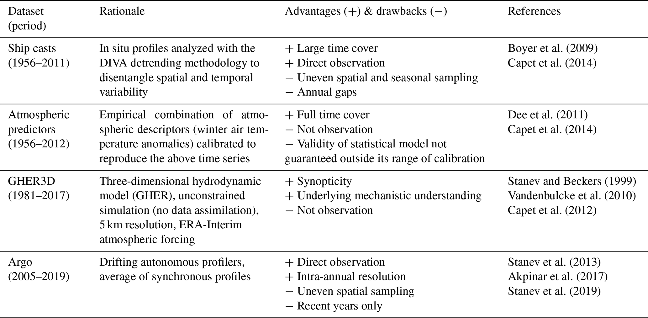
C has been estimated for each year over the 1955–2019 period using four data sources summarized in Table 1. These sources include in situ historical (ship casts) and modern (Argo) observations, as well as empirical and mechanistic modeling (Fig. 1). Annual and spatial average values for the deep sea (depth >50 m) were derived from each dataset, while considering the errors induced by uneven sampling in the context of pronounced seasonal and spatial variability. Each data source has particular advantages and drawbacks and involves specific data processing to reach estimates of annual and spatial C averages as described below. All processed annual time series are made available in netCDF format in a public repository (see “Data availability”).
Boyer et al. (2009)Capet et al. (2014)Dee et al. (2011)Capet et al. (2014)Stanev and Beckers (1999)Vandenbulcke et al. (2010)Capet et al. (2012)Stanev et al. (2013)Akpinar et al. (2017)Stanev et al. (2019)Table 1 Overview of the four datasets used to characterize the CIL inter-annual variability. Details are provided for each dataset in Sect. 2.1.
-
In situ ship-cast profiles. The advantage of ship-based profiles is their extended temporal coverage. The drawbacks are the difficulty to untangle spatial and temporal variability (as for any non-synoptic data source), the uneven sampling effort, and the low data availability posterior to 2000. The CShips time series was provided by the application of the DIVA detrending methodology on ship-cast profiles extracted from the World Ocean Database (Boyer et al., 2009) in the box 40–47∘30′ N, 27–42∘ E for the period 1955–2011. DIVA is sophisticated data interpolation software (Troupin et al., 2012) based on a variational approach. The detrending methodology (Capet et al., 2014) provided inter-annual trends, here representative of the central basin, cleared from the errors induced by the combination of uneven sampling and pronounced variability along the seasonal and spatial dimensions. We redirect the reader to Capet et al. (2014) for further details on data sources, data distribution and methodology.
-
Atmospheric predictors. The statistical model considered here consists of a lagged regression model based on winter air temperature anomalies, i.e., using the form , where i is a year index and ATWi stands for the anomaly of the preceding winter air temperature (December–March).
This model was obtained by a stepwise selection among potential descriptor variables (including summer and winter air temperature, winds, and freshwater discharge), in order to reproduce the inter-annual variability in CShips (Capet et al., 2014) and proposed as an alternative to the winter severity index defined by Simonov and Altman (1991). CAtmos is thus naturally representative of the same quantity, i.e., annually and spatially averaged C. The advantage of this approach is the opportunity to fill the gaps between observations in past years, using atmospheric reanalysis of 2 m air temperature provided by the European Centre for Medium-Range Weather Forecasts (ECMWF) for the period 1980–2013. Its drawbacks lie in its empirical nature and indirect relationship to observable sea conditions. CAtmos was only extracted for the years covered in Capet et al. (2014), considering that the potential non-linearity in the air temperature–C relationship may be exacerbated for the low C values typical of recent years.
-
Three-dimensional (3D) hydrodynamic model. The Black Sea implementation of the 3D hydrodynamic model GHER has been used in several studies (Grégoire et al., 1998; Stanev and Beckers, 1999; Vandenbulcke et al., 2010). In particular, Capet et al. (2012) present the model setup used in this study and analyze the simulated CIL dynamics. This simulation, extending over the period 1981–2017, has been produced without any form of data assimilation, on the basis of the ERA-Interim set of atmospheric forcing provided by the ECMWF data center (Dee et al., 2011). Aggregated weekly outputs of the GHER3D model are made available on a public repository (see “Data availability”). CModel3D was derived from synoptic weekly model outputs and averaged for each year and spatially over the deep basin (depth >50 m). The advantages of this approach are the synoptic coverage in time and space and the mechanistic nature of the model, which implies a reproducible understanding of the process of CIL formation. A drawback lies in the numerical and conceptual error that might affect unconstrained model outputs.
-
Argo profilers. The advantages of autonomous Argo profilers are a high temporal resolution and the continuous coverage of recent years, which offer unprecedented means to explore the CIL dynamics at fine spatial and temporal scales (Akpinar et al., 2017; Stanev et al., 2019). The drawbacks are the mingled spatial and temporal variability inherent to Argo data, the incomplete spatial coverage, and the lack of data prior to 2005. This dataset was collected and made freely available by the Coriolis project and programs that contribute to it (http://www.coriolis.eu.org, last access: 3 March 2020). The request criteria used were as follows: bounding box – 40–47∘ N, 27–42∘ E; period (DD/MM/YYYY) – between “01/01/2005” and “31/12/2019”; data type(s) – “Argo profiles”, “Argo trajectory”; required physical parameters – “sea temperature” or “practical salinity”; quality – good. On average, this set includes about 9 floats per year, with a minimum of 2 floats for 2005 and more than 12 floats from 2013 to 2019. C values were derived from individual Argo profiles (Fig. 1). All available profiles in a given year were averaged to produce the annual Argo time series CArgo. Although homogeneous seasonal sampling can be assumed, we note that the uneven spatial coverage of Argo profiles might induce a bias in the inferred trends. This potential bias stems from the horizontal gradient in C, that is structured radially from the central (lower C) to the peripheral (higher C) regions of the Black Sea (Stanev et al., 2003; Capet et al., 2014). As Argo samplings are generally more abundant in the peripheral regions, i.e., outside of the divergent cyclonic gyres, this suggests that CArgo might be slightly biased towards high values.
With the exception of the pair and , all datasets either are strictly independent or can be considered as such (see Table A1). A composite time series was constructed as the weighted average of the four time series, restricted to available sources for years during which all sources were not available:
where i is an annual index, j stands for a source index (j∈{Model3D, Atmos, Argo, Ships}). In order to emphasize the value of direct observations, the weights () equal 1 if () is defined (i.e., the time series covers the year i) and is 0 otherwise, while () equals 0.5 if () is defined and is 0 otherwise.
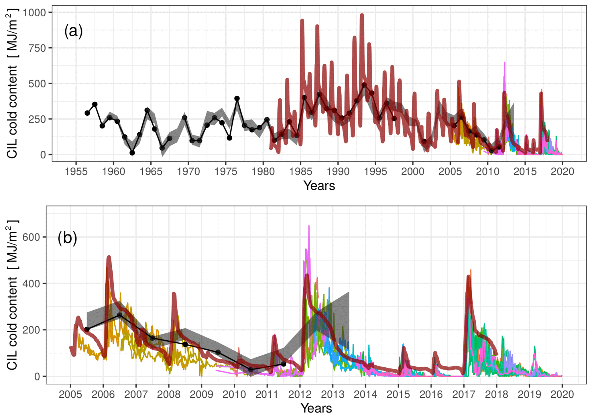
Figure 1 Time series of the Black Sea CIL cold content (C) originating from various data sources (Table 1), displayed at original temporal resolution: (black dots) inter-annual trend derived from ship casts; (gray-shaded area) confidence bounds (p<0.01) of the statistical model based on winter air temperature anomalies; (thick dark red line) GHER3D model; (thin colored lines) individual Argo floats. (a) Complete period of analysis, (b) focus on recent years.
The composite time series was then used as a synoptic metric for the inter-annual variability in the convective ventilation of the Black Sea intermediate layers. The consistency of the different CIL cold-content data sources is demonstrated by the high correlations obtained between the annual time series (from 0.91 to 0.98; see detailed comparative statistics in Appendix A). Despite the small number of overlapping years between certain series (e.g., 7 years between and ; see Fig. A1), all correlations are significant (p<0.05). The close correspondence between independent time series, issued respectively from strictly observational and purely mechanistic modeling approaches provides a high confidence in their accuracy and ensures the robustness of the forthcoming analysis.
More precisely, the standard deviations estimated from the different series are similar (∼100 MJ m−2), despite their distinct temporal coverage. The root-mean-square errors that characterize the disagreement between the different data sources remain below this temporal standard deviation (in all but one case; see Appendix A for details). This justifies merging the different sources into a unique composite time series, enabling a robust long-term analysis of the variability in the Black Sea CIL formation.
2.2 Regime shift analysis and descriptive model selection
The inter-annual variability in the Black Sea CIL formation is analyzed in the framework of regime shift analysis. The natural first step towards identification of a regime shift in a time series is the identification of change points (Andersen et al., 2009).
The rationale behind change point models is to identify periods over which a time series depicts statistically distinct regimes. In its simplest form, a change point model will aim to identify distinct regimes that differ in terms of their mean, i.e., during which fluctuations take place around distinct averages. Note that other types of change point analyses can be done, which would consider other metrics (variance, autocorrelation, skewness) instead of the mean to break up the series. For the sake of simplicity, only the first moment (mean) is considered in this study.
The change point model used for this regime shift analysis has been derived and verified (Appendix B) following the methodology described in the documentation of the R package strucchange (Zeileis et al., 2003).
The procedure includes the following steps.
First, the presence of at least one significant change point in the time series was tested against the null hypothesis that considers annual fluctuations around a fixed average value for the entire time series.
To this aim, the strucchange package provides different methods based on the generalized fluctuation test framework as well as from the F-test (Chow test) framework.
Second, the locations of the most likely change points in the time series were identified. Assuming that N change points separates N+1 periods, this step thus consists in identifying the locations of the change points and the mean value specific to each period. This identification proceeds from an optimization procedure aiming to minimize the residual sum of squares (RSS) between the time series and the change point model (i.e., constant mean value for each specific period).
Five change point models were derived for the composite time series, considering from one (N=1) to five (N=5) change points. The final step consists in selecting, among those five models, the one that “best” describes the time series, obviously considering additional change points can only reduce the RSS. This is generally true for any descriptive model and has led to the definition of the Akaike information criterion (AIC) for model selection. Basically, the AIC considers the RSS of each model but includes a penalty for the number of parameters (Akaike, 1974), such that if two models bear the same RSS, the one involving fewer parameters will be favored. Note that in our case, the parameters identified for change point models include both the locations of change points and the specific mean for each period. The model with the smallest AIC should be favored for interpretation. In Sect. 3.1, the AIC is also used to compare the regime shift models to linear and periodic models of Ci.
More technical details and verification of underlying assumptions are given in Appendix B.
2.3 Oxygen
Biogeochemical Argo (BGC-Argo) oxygen observations were obtained from the Coriolis data center for a period extending from 1 January 2010 to 1 January 2020. Only descending Argo profiles were considered, to minimize discrepancies associated with oxygen sensor response time (Bittig et al., 2014). To minimize the impact of spatial variability, oxygen saturation was considered using a potential-density anomaly (σ) vertical scale, and the year 2010 was discarded for lack of observations. While both oxygen concentration (µM) and oxygen saturation (%) were considered in our first analyses, the narrow range of thermo-haline variability in the layers of interest results in very small variations in the oxygen solubility. As a consequence, considering one or the other of these two variables led to very similar results, and we opted for oxygen saturation in the following.
Figure 2 indicates that the use of σ vertical coordinates minimizes the range of spatial variability (see years 2014–2018, when more Argo floats were operating) and justifies the use of monthly medians as an integrated indicator of the basin-wide oxygenation status at different layers. For deeper density layers (Fig. 2c), a larger interquartile range is induced by Argo floats profiling in the vicinity of the Bosporus-influenced area, as plumes of Bosporus ventilation introduce a larger horizontal variability in oxygen saturation.
3.1 Descriptive models
The composite time series Ci is depicted in Fig. 3, along with individual components.
The poor statistics associated with a linear-model description of Ci, in the form (i stands for an annual index; adjusted R2=0.05; AIC = 794, with MJ m−2 yr−1), cause the perception of a linear trend extending over the entire period to be dismissed. Using the periodic model, , gives a better representation of the cold-content inter-annual variability (AIC = 763), and provides broad characteristics of Ci: the mean value, MJ m−2; the amplitude of inter-annual variability, MJ m−2; and the periodicity of pseudo-oscillations, years.
A combination of linear and periodic models, with the form , slightly improves the descriptive statistics (AIC = 758.5). However, all of the above descriptive models overestimate C in recent years, as the composite time series Ci shows a departure from its usual range of variability during the last decade. This is evidenced by ranking the 65 years of Ci on the basis of their cold content. It is remarkable that, of the 10 years with the least cold content, 8 occurred after 2010.
Each of the change point models appears to be statistically more informative, sensu AIC, than a linear or periodic interpretation of the time series. In particular the four-segment model (i.e., three change points, AIC = 752) should be favored for interpretation.
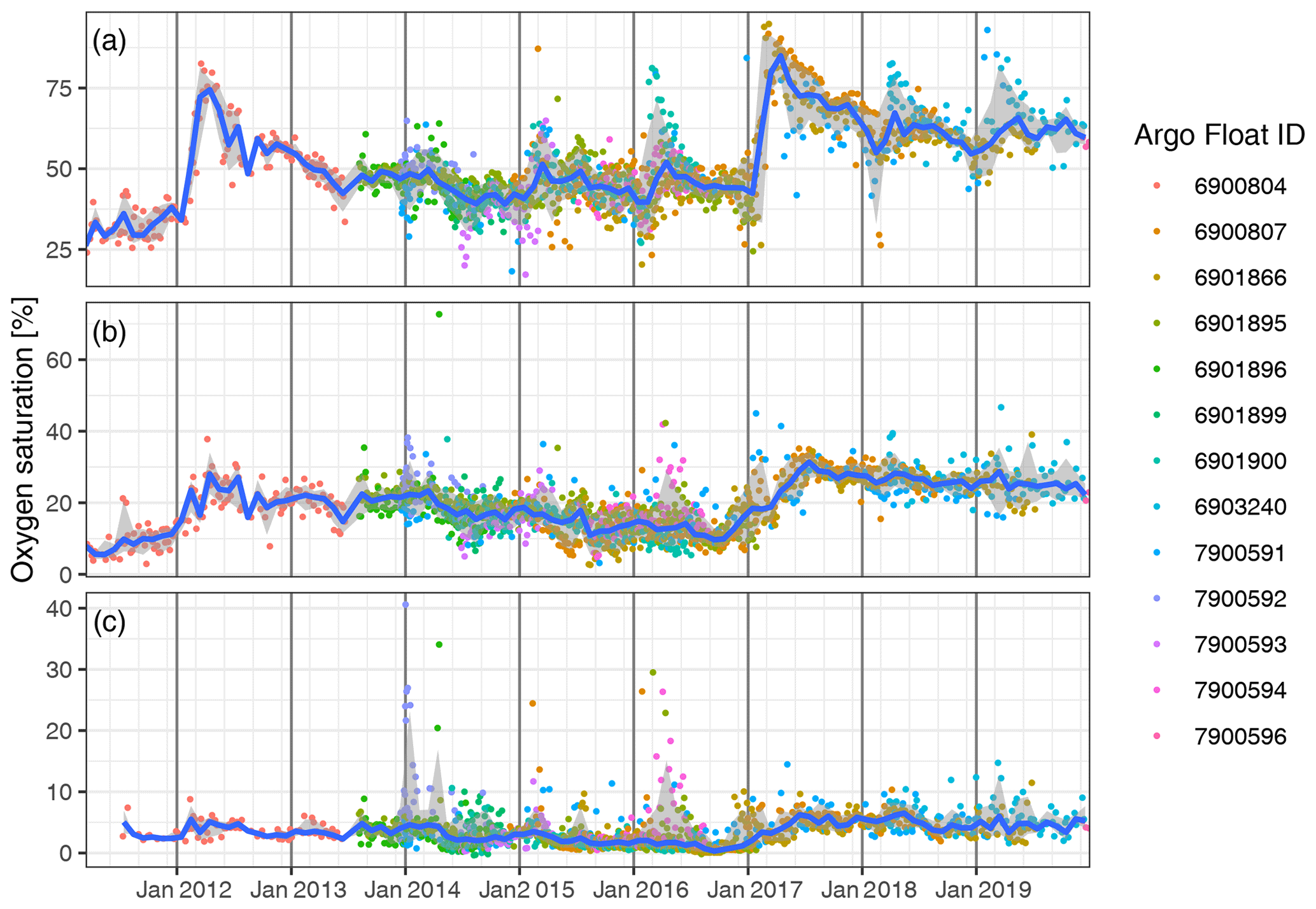
Figure 2 Oxygen saturation levels derived from individual BGC-Argo profiles at σ values of (a) 14.5, (b) 15.0 and (c) 15.5 kg m−3. Colored points correspond to different Argo floats. The blue line represents monthly medians, while the shaded area covers monthly interquartile ranges.
3.2 Regime shifts in the cold-intermediate-layer cold content
The evolution of Ci over 1955–2019 is thus best described by discriminating four periods (P1–P4, Fig. 3), objectively identified through regime shift analysis.
A “standard regime” is identified that is consistent for periods P1 (1955–1984) and P3 (1999–2008), which gives averages MJ m−2 and MJ m−2, respectively. This regime is also consistent with the average C obtained without considering any change points, MJ m−2 (Fig. 3).
Departing from this routine, a cold period (P2) is visible from 1985 to 1998, during which C fluctuates around a larger average value, MJ m−2. This cold period has been described in numerous studies (e.g., Ivanov et al., 2000; Oguz et al., 2006) and is attributed to strong and persistent anomalies in atmospheric teleconnection patterns (East Atlantic–West Russia and North Atlantic oscillations; Kazmin and Zatsepin, 2007; Capet et al., 2012). Noteworthy is that similar cold periods were identified earlier in the 20th century (late 1920s–early 1930s and early 1950s; Ivanov et al., 2000).
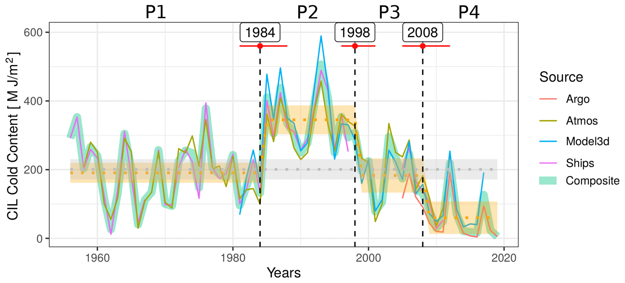
Figure 3 Multi-decadal variability in the Black Sea CIL cold content and distinct periods identified by the regime shift analysis (P1–P4). Confidence intervals for mean C values are indicated by the orange-shaded area for each period and by the gray-shaded area for the null hypothesis (i.e., considering no regime shifts). Confidence intervals for the time limits of each period are indicated with red error bars.
From 2009 to 2019, a warmer period (P4) is identified during which C varies around a lower average MJ m−2. The regime shift analysis thus evidences a general weakening of the cold-water formation and associated ventilation that has prevailed in the Black Sea for about 10 years. Warm years and low cold content were also observed during the years 1961 and 1963, but those were not identified as part of a statistically distinct “warm” regime and should be considered strong fluctuations within P1. The regime shift analysis thus indicates that the current restricted ventilation conditions have no precedent in modern history.
The intra-annual resolution provided by the 3D model and Argo time series (Fig. 1) suggests that the partial CIL renewal, which was taking place systematically each year before 2009, has now become occasional. Here we focus on period P4, better detailed in our datasets, to characterize the CIL formation as a basin-wide ventilation process and its relationship with changes in oxygen saturation at different σ levels.
Basin-wide CIL formation and destruction rates were computed from the synoptic 3D model outputs, as differences between weekly C values (Fig. 4). The seasonal sequence depicts CIL formation peaks from late December to March, typically reaching C formation rates of 5, 10 and 1 MJ m−2 d−1 for the period P1–P3, P2 and P4, respectively (Fig. 4a–c). The CIL cold content is then eroded at different rates before, during and at the end of the thermocline season, with a damped erosion rate through the thermocline season between 0 and about 1 MJ m−2 d−1. CIL formation processes have been described extensively in the past (e.g., Akpinar et al., 2017; Miladinova et al., 2018), in more detail than is allowed by the integrated perspective adopted here. This integrated point of view, however, serves to point out the striking quasi-absence of CIL formation peaks for the years 2001, 2007, 2009, 2010, 2013 and 2014 (Fig. 4d). In fact, during the period of Argo oxygen sampling (2011–2020), only 2012 and 2017 depict important CIL formation events, while minor CIL formation events are shown for 2015 and 2016.
Oxygen saturation in this period varies in concordance with CIL formation up to σ layers of about 16.0 kg m−3 (Fig. 5). Large increases can be observed from December to March in the years 2012, 2015, 2016 and 2017 when CIL formation is significant, which denotes the impact of convective ventilation. The narrow interquartile ranges depicted in Fig. 5 denote the efficiency of the isopycnal diffusion of oxygen: the amount of oxygen imported with the newly formed CIL waters is distributed horizontally and contributes to increasing the average oxygen saturation of a given σ layer.
While major CIL formation events in 2012 and 2017 induced a significant increase in oxygen saturation through the whole oxygenated water column, the minor events in 2015 and 2016 seem to have had a limited penetration depth. For instance, oxygen saturation at 14.6 kg m−3 only stagnates during 2015 and 2016 as compared to 2014, while oxygen saturation at 15.1 kg m−3 keeps decreasing during these 2 years, indicating that the amount of oxygen brought to this layer during minor ventilation events is not sufficient to counterbalance the biogeochemical oxygen consumption terms (i.e., respiration and oxidation of reduced substances diffusing upwards).
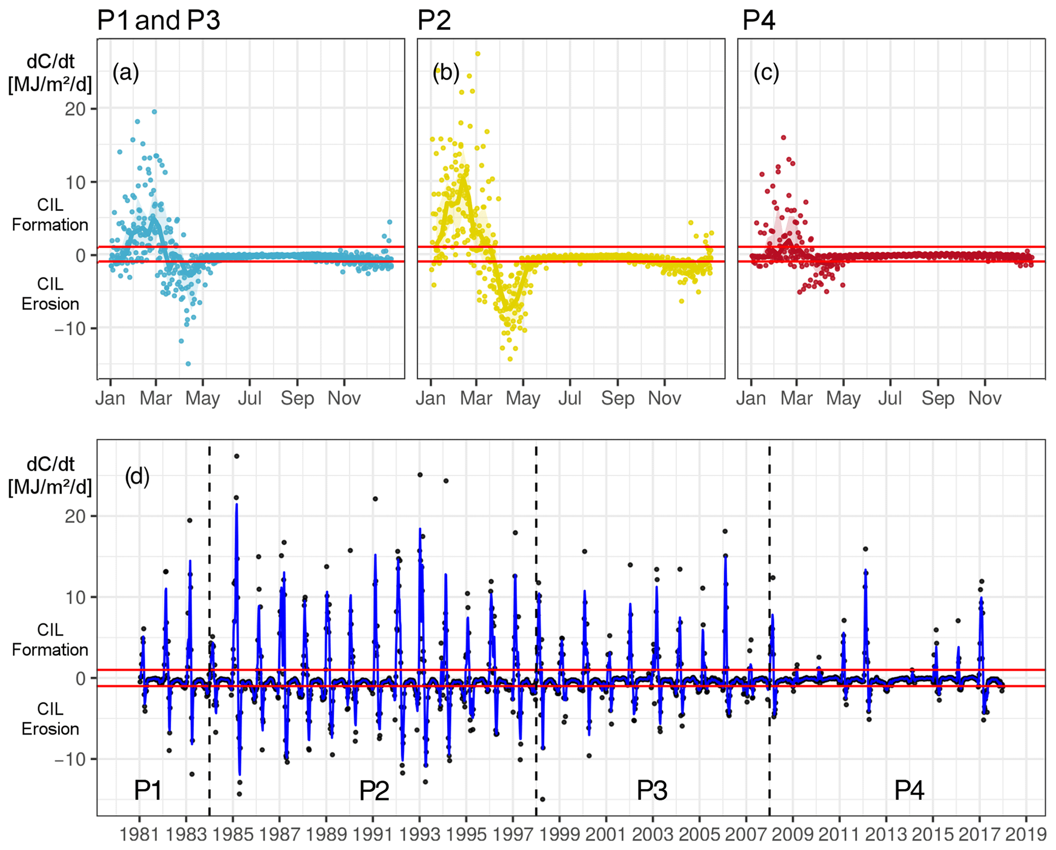
Figure 4 Weekly averaged basin-wide CIL cold-content formation and destruction rates (dC∕dt), obtained as differences between the weekly integrated CIL cold content provided by the GHER3D model: (a–c) in a seasonal frame with weekly medians (line) and interquartile range (shaded area), merging years from the periods P1 and P3 (considered together), P2, and P4; (d) on an inter-annual scale, with a 3-week running average (blue line). Vertical dashed lines separate the four periods identified by the regime shift model. The red lines delineate the thresholds of ±1 MJ m−2 d−1, corresponding to the lower bound of the CIL erosion rate during summers.
Following our attempt to summarize large datasets and to characterize a basin-scale annual oxygenation rate, we computed for each layer an annual oxygenation index as the difference between the median oxygen saturation in November between successive years. The rationale behind this approach is that CIL formation typically extends from December to March (Fig. 4a–c).
In order to obtain a general indication of the (pycnal) penetration depth of the convective ventilation associated with CIL formation, we assessed the Pearson correlation coefficient between this annual oxygenation index and a first-order assessment of annual CIL formation, obtained as the annual difference in the C composite time series. The correlation between oxygenation and CIL formation is high near the surface and decreases continuously as deeper pycnal levels are considered. Those correlations remain significant (p<0.1) until σ=15.4 kg m−3 (Fig. 6).

The regime shift paradigm describes an abrupt and significant change in the observable outcome of a non-linear system, as could result from a threshold in this system response to external forcing. In contrast, a periodic model supposes either a linear response to periodically varying external forcing or an oscillation resulting from internal dynamics. It is our hypothesis, supported by the quantitative analysis presented in this study, that the regime shift model should be favored for interpreting the recent evolution of the Black Sea CIL dynamics. The prerequisite for the regime shift analysis was first to issue an unified, synoptic metric to characterize inter-annual variations in the CIL content. The consistency between the different data sources used to construct this metric demonstrates the robustness of this metric. To our knowledge, no multi-source comparison has been previously achieved over such an extended period. Note that some dependencies exist among certain sources, as discussed explicitly in Table A1.
Although we acknowledge that the statistical advantage (AIC) of the regime shift description is subtle, we consider that it deserves further consideration as this difference in interpretation is fundamental in regards to the expected consequences on the Black Sea oxygenation status and in particular the threat to Black Sea marine populations, whose ecological adaptation (and rate of exploitation) has been built upon a ventilation regime and consequent biogeochemical balance that may no longer prevail.
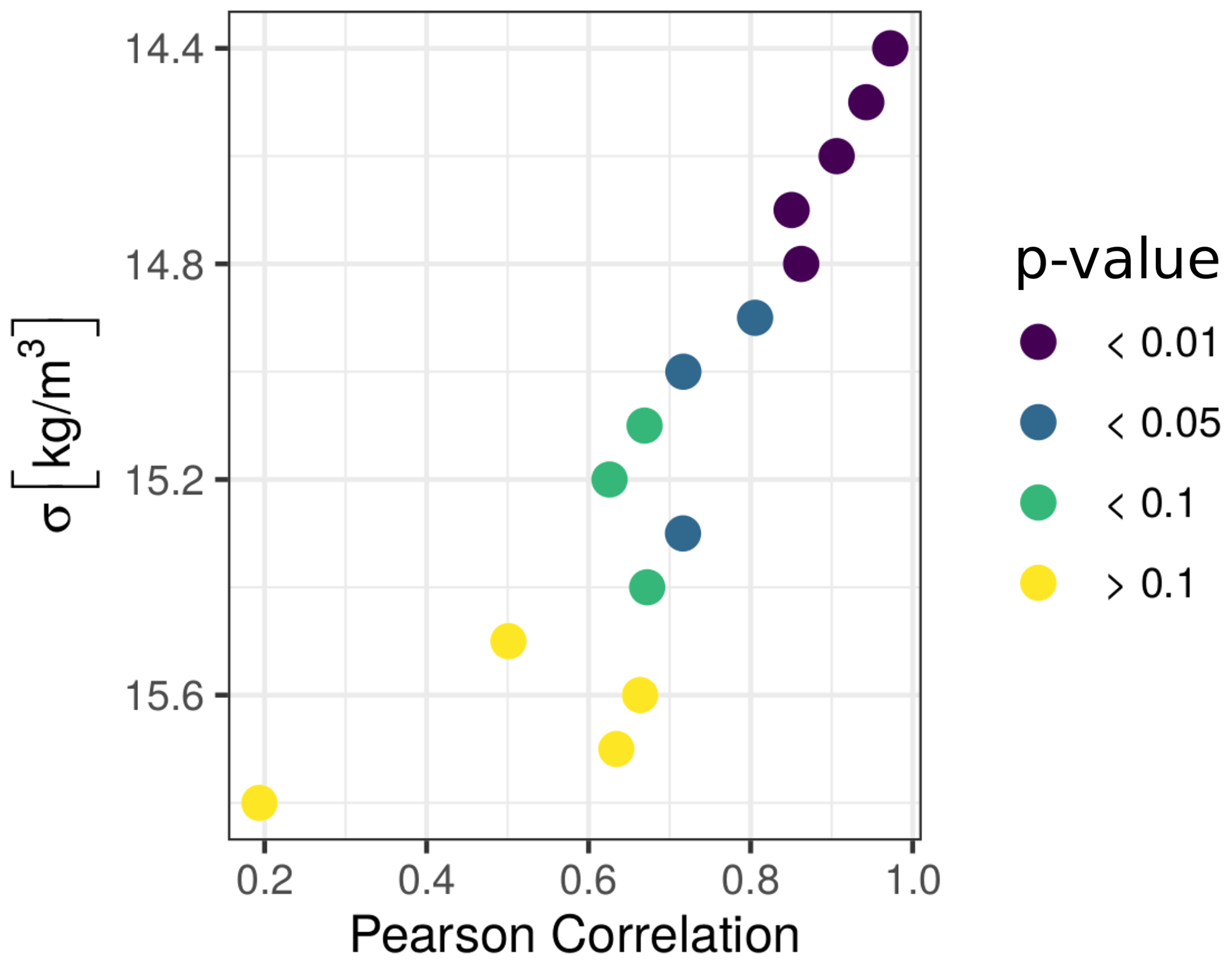
Figure 6 Pearson correlation coefficient between basin-wide annual oxygenation and CIL formation estimates for different σ layers. Color of the points relates to the order of magnitude of associated p values.
Indeed, it appears that the intermittency of significant CIL formation events characterizes the new ventilation regime: the ventilation of the Black Sea intermediate layers does not occur each year anymore but is occasionally absent for 1 or 2 consecutive years. Moreover, major CIL formation events, which bear the potential for deeper oxygenation, appear significantly less frequently.
The extent to which the current regime differs from the previous ventilation regimes is clearly illustrated on a T–S diagram:
in situ measurements from period P4 are commonly found in a range of the T–S diagram (T>8.35 ∘C and σ within 14.5–15 kg m−3) that was extremely rare in previous periods (see density contours on Fig. 7a–d; two-dimensional density estimates were obtained with the R function MASS:kde2d).
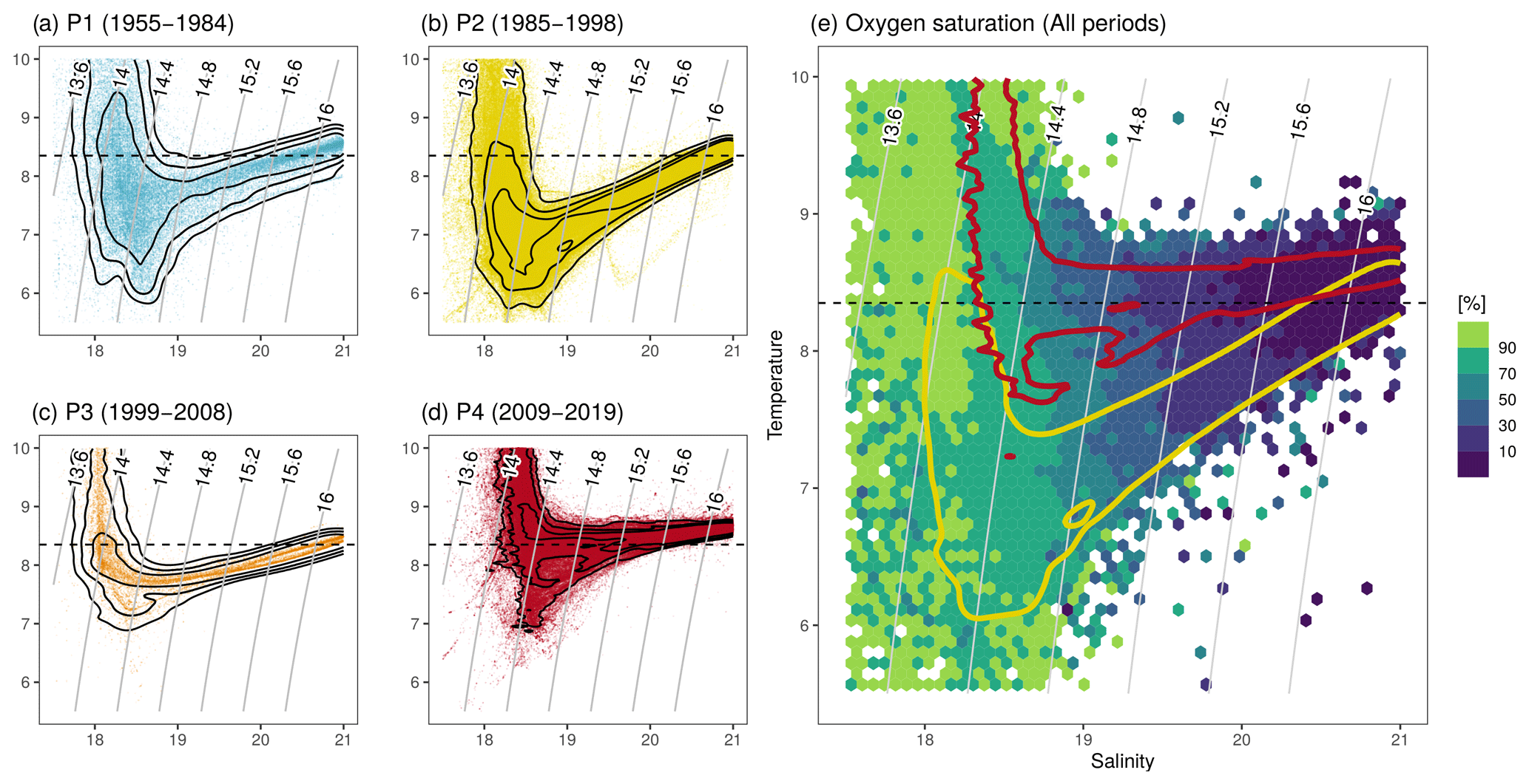
Figure 7 (a–d) Potential temperature versus salinity (T–S diagram) for bottle, CTD and Argo in situ data available from the World Ocean Database for the period 1955–2020 (Boyer et al., 2018). Data from periods P1, P2, P3 and P4 are shown in (a)–(d), respectively. Black contours delineate 90 %, 75 % and 50 % of the observations for each period. (d) Historical oxygen records collected from the World Ocean Database for the period 1955–2020 (Boyer et al., 2018), averaged for hexagonal bins of the T–S diagram. The 75 % contour of P2 (yellow) and P4 (red) are repeated to highlight the difference in oxygenation state at a given density between the two corresponding contrasted CIL regimes. For all panels, the isopycnal σ layers are indicated by curved gray lines. The dashed black line locates the TCIL=8.35 ∘C criterion used to identify CIL waters.
As indicated by Stanev et al. (2019), this trend may lead to the disappearance of a characteristic layer of the Black Sea, which constituted a major component of its thermo-haline structure and constrained the exchanges between surface, subsurface and intermediate layers. In particular, the authors highlight surface and subsurface salinity trends that indicate recent occurrences of diapycnal mixing at the lower base of the intermediate layer, where waters are characterized by a strong reduction potential due to the presence of reduced iron and manganese species, ammonium, and finally hydrogen sulfide (Pakhomova et al., 2014).
On a decadal timescale, the average oxygen signature of a given isopycnal layer within the CIL depends on the frequency of CIL formation events of sufficient intensity (Sect. 4), which is in line with the ventilation dynamics described by Ivanov et al. (2000) for the upper pycnocline. Although inter-annual fluctuations in the CIL formation rate still occur, the regime shift analysis specifically describes a reduction in the average CIL cold content, which appears to be associated with a reduction in the frequency of significant ventilation events (Fig. 4) and therefore a potential decrease in the oxygen saturation signature in the lower part of the CIL.
Importantly, this reduction may also affect deeper layers of the Black Sea. Indeed, the mid-pycnocline (σ between about 14.6 and 16 kg m−3) is formed by the two end-member mixing lines between the CIL layer and the Bosporus inflow (Murray et al., 1991; Ivanov et al., 2000), which proceeds from the entrainment of CIL waters by the Bosporus inflow and subsequent lateral ventilation (Buesseler et al., 1991). Considering the characteristic residence time for the upper (about 5 years; Lee et al., 2002) and intermediate (9–15 years; Ivanov et al., 2000) pycnocline, it is appropriate to consider such temporal averages to characterize the oxygen signature of the CIL member composing the mixture of pycnocline waters.
Displaying historical oxygen saturation data (1955–2020) on the T–S diagram (Fig. 7e) indeed shows generally deeper oxygenation during high-CIL regimes than during low-CIL regimes. For instance, oxygen saturation in the density range σ=14.8–15.2 kg m−3 lies in the range of 30 %–70 % in the T–S region that is characteristic of P2, while it only reaches 10 %–50 % in the T–S region characteristic of P4. This indicates that the analysis linking oxygenation and CIL formation for the recent period (Sect. 4) can be extended to larger timescales by considering changes in the frequency of significant CIL formation events. Thus, the depth up to which the reduction in CIL formation may impact on the biogeochemical balance of the Black Sea (by affecting the oxygenation level) will depend on the period over which the current ventilation regime will continue.
Indeed, it is important to highlight that the current regime may not necessarily be a new steady regime – even though it has been identified as such by the change point analysis – but that it could be part of a transient downwards trend that started in the mid-1990s. The reason why it appeared important to us to oppose non-linear regime dynamics with smooth linear and sine trend models is that the recent CIL dynamics, when depicted by the regime change approach, is not slow-trending but suggests a step change towards a new phenology for the intermediate Black Sea. Only future observations may now confirm or invalidate the relevance of the proposed regime shift paradigm.
Beyond the changes in convective ventilation highlighted above, it thus appears as a lead priority to assess the biogeochemical consequences of this new thermo-haline dynamics of the Black Sea. In particular, the influence of CIL formation on the biogeochemical components of the oxygen budget should be addressed in more detail, asking for instance how the presence or absence of CIL formation influences planktonic growth, trophic interactions and organic-matter respiration rates. We voluntarily adopted here a wide integrative point of view so as to highlight the large-scale relevance of the identified regime shift to Black Sea oxygenation. However, we still consider that a detailed assessment of all components of the oxygen budget, i.e., ventilating processes and biogeochemical terms, is required in order to infer the future evolution of the Black Sea oxygenation status (e.g., Grégoire and Lacroix, 2001).
Although there are clear indications of a long-term warming trend in the Black Sea (Belkin, 2009), it remains a delicate task to strictly dissociate the contributions of global warming from those of regional atmospheric oscillations (Kazmin and Zatsepin, 2007; Capet et al., 2012). One such assessment in the neighboring Mediterranean Sea (Macias et al., 2013) concluded that global warming trend and regional oscillation contributed 42 % and 58 % of the recent regional sea surface temperature trend (1985–2009), respectively. While a corresponding assessment will have to be routinely reevaluated for the Black Sea as the time series expands, it may conservatively be considered that global warming has made a significant contribution to warming winters in the Black Sea. This contribution is expected to increase in the next decades (Kirtman et al., 2014).
We have analyzed the variability in the Black Sea CIL formation over the last 65 years and investigated the existence of regime shifts in this dynamics. For this purpose, we have produced a composite time series of the CIL cold content (C) that is considered a proxy for the intensity of the convective ventilation resulting from the formation of dense oxygenated waters. This composite time series is built from four different data products issued from observations and modeling so as to optimize its temporal extent in regards to preceding studies (e.g., Oguz et al., 2006). The consistency between those products and in particular the close correspondence between observational and mechanistic predictive time series supports the reliability of the composite series and its adequacy to describe the evolution of the Black Sea subsurface convective ventilation during the last 65 years.
The composite time series was analyzed to detect different regimes, corresponding to periods characterized by significantly distinct averages. We identified three main regimes that have existed over last 65 years: (1) a standard regime prevailing during 1955–1984 and 1999–2008 that is consistent with the full-period average C, (2) a cold regime (high C, 1985–1998) which has been previously documented (see references in Sect. 3), and (3) a warm regime (low C, 2009–2019) which is characterized by the intermittency of the annual partial CIL renewal. Statistical considerations indicate that the abrupt shift can not adequately be described by a combination of long-term linear and periodic trends. However, monitoring the future evolution of the CIL is necessary to confirm that this abrupt-change description should be favored over that of a transient dynamics.
The synoptic CIL formation rates provided by the 3D hydrodynamic model and the detailed description of oxygenation conditions provided by BGC-Argo floats allowed us to detail the role of CIL formation in oxygenating the upper part of the Black Sea intermediate layers through convective ventilation (i.e., σ of between 14.4 and 15.4 kg m−3). Given that cold winter air temperature is the leading driver of CIL formation (Oguz and Besiktepe, 1999; Ivanov et al., 2000; Capet et al., 2014); given that CIL formation constitutes a dominant ventilation mechanism for the Black Sea intermediate layer; and assuming that oxygen conditions constitute an environmental structuring factor affecting the ecosystem organization, its vigor and its resilience (Breitburg et al., 2018), this shift in the Black Sea ventilation regime may be associated with global warming and is expected to affect its biogeochemical balance and to threaten marine populations adapted to previously prevailing ventilation regimes.
To understand how global warming impacts marine deoxygenation dynamics is a worldwide concern. The relatively fast and clear response that stems from the specific Black Sea geomorphology makes it a natural laboratory to study this dependency and related phenomena, although the specificity of this morphology also limits the direct transposition of Black Sea results to the global ocean. Here, we showed that non-linear dynamics and feedbacks in ventilation mechanisms resulted in a significant shift in the average ventilation regime, in response to rising air temperature. Since the temporal extent of low-oxygen conditions is critical for ecosystems, we stress the importance of assessing the potential for similar ventilation regime shifts in other oxygen-deficient basins.
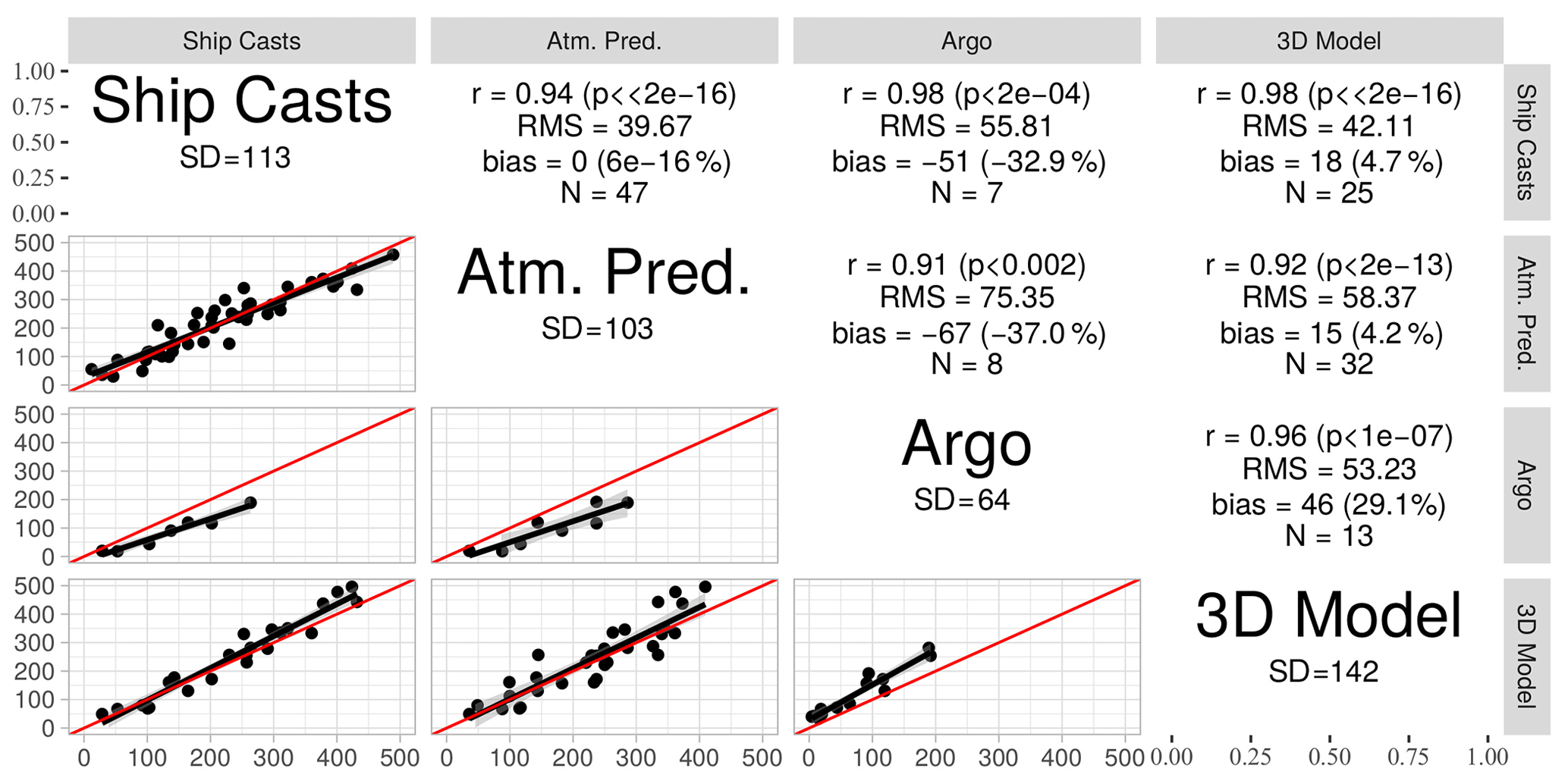
Figure A1 Statistics of comparison between the different data sources: Pearson correlation coefficient (r), root-mean-square deviation (RMS), average bias (bias); number of overlapping years between time series (N) and, on diagonal elements, the standard deviation of each time series (SD).
The C time series are denoted for source m (i is the year index). Each pair of time series (, ) are compared over the years for which and are both defined. The following statistics are given for each pair of data sources in Fig. A1:
-
Nm,n, the number of elements in Im,n;
-
Pearson correlation coefficient,
-
the root-mean-square deviation between time series,
-
the average bias,
-
the percentage bias,
For a better appreciation of variation scales, the temporal standard deviation is also shown for each data source.
The last value of the atmospheric predictor time series (; Fig. 1) was not considered in the composite time series, as it was based on the two, rather than three, predictor values available at the time of publication (hence the larger associated uncertainty). It is remarkable, however, that the published prognostic values for 2012 and 2013 match with independent Argo estimates (Capet et al., 2014).
Finally, Table A1 provides specific comments on the dependence relationship between the different time series presented above. Only and can be considered strictly dependent. is influenced by the same datasets that were used to build and but through drastically different processing pathways and can thus be considered practically independent.
Table A1Dependence relationships between the different datasets.

Table A2 Tests for the presence of significant structural changes in Ci. The p value indicates the probability that the null hypothesis (i.e., there are no significant change points) should be maintained. All tests, except that highlighted in bold, indicate the presence of significant structural changes in Ci with a confidence level higher than 95 %.
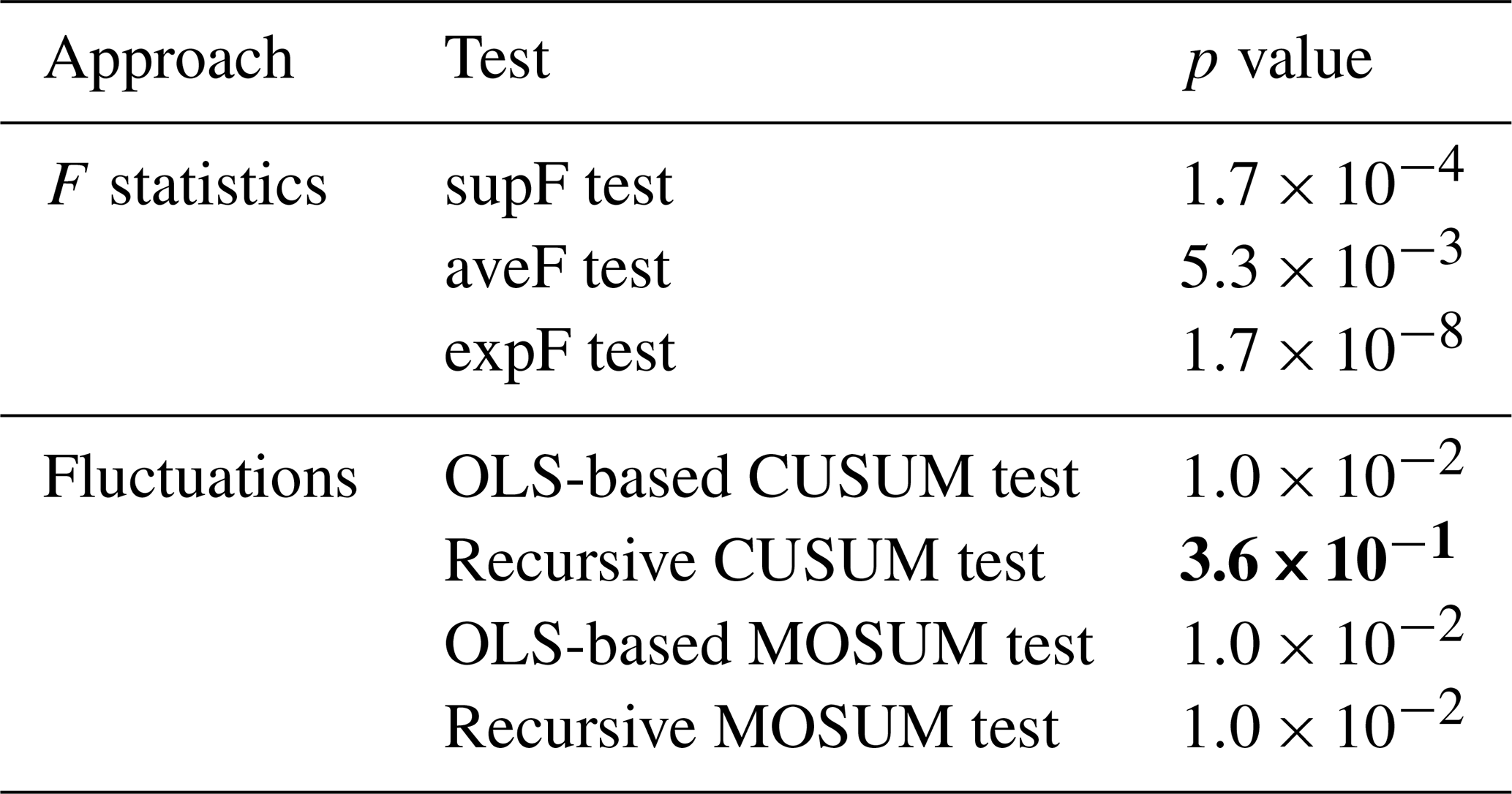
Table A3 Correlations between (second column) time-lagged replicates of the original Ci and (third column) time-lagged replicates of the residuals of the four-segment model.

The basic change point problem that is considered in this study can be expressed as follows: to identify the change point i=k in a sequence xi of independent random variables with constant variance, such that the expectation of xi is μ for i<k and μ+Δμk otherwise.
Obviously, this problem can be generalized for several change points.
The procedure for change point detection is stepwise and has been achieved following the methodology described in the documentation of the R package strucchange (Zeileis et al., 2003).
First, the existence of at least one significant change point had to be tested. The package
strucchange provides seven statistical tests to compute the p value at which the null hypothesis of no change points can be rejected.
The presence of change points can be tested on the basis of F-statistic tests or generalized fluctuation tests (Zeileis et al., 2003, and
references therein).
Table A2 provides the significance level at which the null hypothesis can be rejected for each test implemented in the strucchange R package.
Among the seven tests considered to assess the presence of at least one significant change point in Ci, six reject the null hypothesis with a significance level p<0.05.
Second, the locations of the N most likely change points were identified. In this study, we considered from one to five change points. The change point locations can be estimated by finding the index values that maximize a likelihood ratio, defined as the ratio of the residual sum of squares for the alternative hypothesis (i.e., change points at kn with ) to that of the null hypothesis (i.e., no change point, ).
Formally, the methodology to identify and date structural change is designed for normal random variables, two conditions which can not be guaranteed for environmental time series such as those considered here. We detail here why (1) the departure of C distribution from a Gaussian distribution, (2) the autocorrelation in the composite time series Ci and (3) the biases between source-specific components of Ci do not affect the conclusions drawn above.
B1 Normality
Skewness in the distribution of C values and its departure from normality is visible at low C values (not shown), as expected for physical reasons: C is a vertically integrated property, naturally bounded by zero. However, the Shapiro–Wilk test that measures the correlation between the quantiles of Ci and those of a normal distribution indicates no significant departure from normality: W=0.975, p=0.23. For completeness, a Box–Cox transformation (λ=0.7) of the original data has been tested which slightly enhances the Shapiro–Wilk test (W=0.98, p=0.39) but brings no sensible alteration in the conclusions of the structural-change analysis.
B2 Autocorrelation
Similarly, Ci can not be considered a random variable. In particular, we introduced in Sect. 1 the CIL preconditioning and partial renewal mechanisms, both physical reasons for which autocorrelation may be expected in Ci. Indeed, correlations between the original and k-lagged time series are, at first glance, significant up to k=5 (Table A3; the confidence interval above which autocorrelation can be considered to be significant is given by ). However, it should be considered that the regime shift evidenced in this study may itself induce apparent autocorrelation statistics. To evidence that this is indeed the case encountered here, the correlations between the original and lagged time series of the residuals stemming from the four-segment change point model are indicated in Table A3. The fact that no significant autocorrelation persists when change points are considered indicates that the non-randomness of Ci does not jeopardize conclusions drawn from the application of the structural-change methodology.
B3 Biases between components of the composite time series
Given that biases exist between different data sources, it might be argued that the composite time series is skewed by the uneven temporal coverage of the different sources. For instance, if a strongly biased source were to solely cover a given period, the composite series would be biased over that period. To ensure that this issue does not affect the presented conclusions, was constructed as Ci but removing from each component , the bias identified with the longest time series (which series is used for reference does not impact on structural-change conclusions). When is considered instead of Ci, similar results are obtained in terms of change point model significance and positions of the change points.
The data used are listed in Table 1. Argo data were collected and made freely available by the Coriolis project (http://www.coriolis.eu.org/, last access: 3 March 2020, IFREMER, 2020) and programs that contribute to it. Era-Interim atmospheric conditions were obtained from the ECMWF interface (http://apps.ecmwf.int/datasets/, last access: 1 August 2019, European Centre for Medium-Range Weather Forecasts, 2019). Aggregated weekly outputs of the GHER3D model, as well as processed annual time series from the different sources, are publicly available in a Zenodo repository: https://doi.org/10.5281/zenodo.3691960, last access: 28 February 2020, Capet et al., 2020.
AC processed the data, set the regime shift methodology, achieved the analyses, issued the visualizations, and wrote the initial version and revisions of the manuscript. All authors contributed to defining the general methodology, to discussing the results and to revising the final manuscript. MG supervised the research.
The authors declare that they have no conflict of interest.
This article is part of the special issue “Ocean deoxygenation: drivers and consequences – past, present and future (BG/CP/OS inter-journal SI)”. It is a result of the International Conference on Ocean Deoxygenation, Kiel, Germany, 3–7 September 2018.
This study was funded by the Fonds de la Recherche Scientifique (FNRS) and convention BENTHOX (PDR T.1009.15) and directly benefited from the resources made available within the PERSEUS project, funded by the European Commission, grant agreement 287600. Luc Vandenbulcke is funded by the EU Copernicus Marine Environment Service program (contract BS-MFC). Arthur Capet and Marilaure Grégoire are a postdoctoral fellow and research director, respectively, at the FNRS. Computational resources have been provided by the supercomputing facilities of the Consortium des Équipements de Calcul Intensif en Federation Wallonie Bruxelles (CÉCI) funded by the Fond de la Recherche Scientifique de Belgique (FRS-FNRS). Finally, this study was substantially enhanced thanks to the patient revisions proposed by Fabian Große, James W. Murray, Michael Dowd and an anonymous reviewer, to whom we hereby express our deepest gratitude.
This research has been supported by FRS-FNRS.
This paper was edited by Katja Fennel and reviewed by James W. Murray, Fabian Große, Michael Dowd and one anonymous referee.
Akaike, H.: A new look at the statistical model identification, IEEE T. Automat. Contr., 19, 716–723, 1974. a
Akpinar, A., Fach, B. A., and Oguz, T.: Observing the subsurface thermal signature of the Black Sea cold intermediate layer with Argo profiling floats, Deep-Sea Res. Pt. I, 124, 140–152, 2017. a, b, c, d
Andersen, T., Carstensen, J., Hernandez-Garcia, E., and Duarte, C. M.: Ecological thresholds and regime shifts: approaches to identification, Trends Ecol. Evol., 24, 49–57, 2009. a
Belkin, I. M.: Rapid warming of large marine ecosystems, Progr. Oceanogr., 81, 207–213, 2009. a, b
Belokopytov, V.: Interannual variations of the renewal of waters of the cold intermediate layer in the Black Sea for the last decades, Phys. Oceanogr., 20, 347–355, 2011. a, b
Bittig, H. C., Fiedler, B., Scholz, R., Krahmann, G., and Körtzinger, A.: Time response of oxygen optodes on profiling platforms and its dependence on flow speed and temperature, Limnol. Oceanogr., 12, 617–636, https://doi.org/10.4319/lom.2014.12.617, 2014. a
Bopp, L., Le Quéré, C., Heimann, M., Manning, A. C., and Monfray, P.: Climate-induced oceanic oxygen fluxes: Implications for the contemporary carbon budget, Global Biogeochem. Cy., 16, https://doi.org/10.1029/2001gb001445, 2002. a
Bopp, L., Resplandy, L., Orr, J. C., Doney, S. C., Dunne, J. P., Gehlen, M., Halloran, P., Heinze, C., Ilyina, T., Séférian, R., Tjiputra, J., and Vichi, M.: Multiple stressors of ocean ecosystems in the 21st century: projections with CMIP5 models, Biogeosciences, 10, 6225–6245, https://doi.org/10.5194/bg-10-6225-2013, 2013. a
Boyer, T., Antonov, J., Garcia, H., Johnson, D., Locarnini, R., Mishonov, A., Pitcher, M., Baranova, O., and Smolyar, I.: Chapter 1: Introduction, World ocean database, p. 216, 2009. a, b
Boyer, T. P., Baranova, O. K., Coleman, C., Garcia, H. E., Grodsky, A., Locarnini, R. A., Mishonov, A. V., Paver, C. R., Reagan, J. R., Seidov, D., Smolyar, I. V., Weathers, K., and Zweng, M. M.: World Ocean Database 2018, A. V. Mishonov, Technical Ed., NOAA Atlas NESDIS 87, 2018. a, b
Breitburg, D., Levin, L. A., Oschlies, A., Grégoire, M., Chavez, F. P., Conley, D. J., Garçon, V., Gilbert, D., Gutiérrez, D., Isensee, K., Jacinto, G. S., Limburg, K. E., Montes, I., Naqvi, S. W. A., Pitcher, G. C., Rabalais, N. N., Roman, M. R., Rose, K. A., Seibel, B. A., Telszewski, M., Yasuhara, M., and Zhang, J.: Declining oxygen in the global ocean and coastal waters, Science, 359, eaam7240, https://doi.org/10.1126/science.aam7240, 2018. a, b
Buesseler, K. O., Livingston, H. D., and Casso, S. A.: Mixing between oxic and anoxic waters of the Black Sea as traced by Chernobyl cesium isotopes, Deep-Sea Res., 38, 725–745, https://doi.org/10.1016/S0198-0149(10)80006-8, 1991. a
Capet, A., Barth, A., Beckers, J.-M., and Grégoire, M.: Interannual variability of Black Sea's hydrodynamics and connection to atmospheric patterns, Deep-Sea Res. Pt. II, 77, 128–142, https://doi.org/10.1016/j.dsr2.2012.04.010, 2012. a, b, c, d, e, f
Capet, A., Troupin, C., Carstensen, J., Grégoire, M., and Beckers, J.-M.: Untangling spatial and temporal trends in the variability of the Black Sea Cold Intermediate Layer and mixed Layer Depth using the DIVA detrending procedure, Ocean Dynam., 64, 315–324, 2014. a, b, c, d, e, f, g, h, i, j, k, l, m
Capet, A., Stanev, E. V., Beckers, J.-M., Murray, J. W., and Grégoire, M.: Decline of the Black Sea oxygen inventory, Biogeosciences, 13, 1287–1297, https://doi.org/10.5194/bg-13-1287-2016, 2016. a, b
Capet, A., Vandenbulcke, L., and Grégoire, M.: Black Sea cold intermediate layer cold content from in-situ and modelling sources (1955-2019), [Data set], available at: https://doi.org/10.5281/zenodo.3691960, last access: 28 February 2020. a
Coppola, L., Prieur, L., Taupier-Letage, I., Estournel, C., Testor, P., Lefèvre, D., Belamari, S., LeReste, S., and Taillandier, V.: Observation of oxygen ventilation into deep waters through targeted deployment of multiple Argo-O2 floats in the north-western Mediterranean Sea in 2013, J. Geophys. Res.-Oceans, 122, 6325–6341, 2017. a
Dee, D. P., Uppala, S., Simmons, A., Berrisford, P., Poli, P., Kobayashi, S., Andrae, U., Balmaseda, M., Balsamo, G., Bauer, P., Bechtold, P., Beljaars, A. C. M., van de Berg, L., Bidlot, J., Bormann, N., Delsol, C., Dragani, R., Fuentes, M., Geer, A. J., Haimberger, L., Healy, S. B., Hersbach, H., Hólm, E. V., Isaksen, L., Kållberg, P., Köhler, M., Matricardi, M., McNally, A. P., Monge-Sanz, B. M., Morcrette, J.-J., Park, B.-K., Peubey, C., de Rosnay, P., Tavolato, C., Thépaut, J.-N., and Vitart, F.: The ERA-Interim reanalysis: Configuration and performance of the data assimilation system, Q. J. Roy. Meteor. Soc., 137, 553–597, 2011. a, b
European Centre for Medium-Range Weather Forecasts: ECMWF Public Datasets, available at: https://apps.ecmwf.int/datasets/, last access: 1 August 2019. a
Gregg, M. and Yakushev, E.: Surface ventilation of the Black Sea's cold intermediate layer in the middle of the western gyre, Geophys. Res. Lett., 32, 3, https://doi.org/10.1029/2004gl021580, 2005. a, b
Grégoire, M. and Lacroix, G.: Study of the oxygen budget of the Black Sea waters using a 3D coupled hydrodynamical–biogeochemical model, J. Mar. Syst., 31, 175–202, https://doi.org/10.1016/S0924-7963(01)00052-5, 2001. a
Grégoire, M., Beckers, J. M., Nihoul, J. C. J., and Stanev, E.: Reconnaissance of the main Black Sea's ecohydrodynamics by means of a 3D interdisciplinary model, J. Mar. Syst., 16, 85–105, https://doi.org/10.1016/S0924-7963(97)00101-2, 1998. a
IFREMER: Coriolis: In situ data for operational oceanography, available at: http://www.coriolis.eu.org/, last access: 3 March 2020. a
Ivanov, L., Belokopytov, V., Ozsoy, E., and Samodurov, A.: Ventilation of the Black Sea pycnocline on seasonal and interannual time scales, Mediterr. Mar. Sci., 1, 61–74, 2000. a, b, c, d, e, f, g
Kazmin, A. S. and Zatsepin, A. G.: Long-term variability of surface temperature in the Black Sea, and its connection with the large-scale atmospheric forcing, J. Mar. Syst., 68, 293–301, 2007. a, b
Keeling, R. F., Körtzinger, A., and Gruber, N.: Ocean deoxygenation in a warming world, Annu. Rev. Mar. Sci, 2, 199–229, https://doi.org/10.1146/annurev.marine.010908.163855, 2010. a
Kirtman, B., Power, S. B., Adedoyin, J. A., Boer, G. J., Camilloni, I., Doblas-Reyes, F. J., Fiore, A. M., Kimoto, M., Meehl, G. A., Prather, M., Sarr, A., Schar, C., Sutton, R., van Oldenborgh, G. J., Vecchi, G., and Wang, H. J.: Near-term climate change: projections and predictability, in: Climate change 2013: the physical science basis: contribution to the Fifth Assessment Report of the Intergovernmental Panel on Climate Change, edited by: Stocker, T. F., Qin, D., Plattner, G.-K., Tignor, M. M. B., Allen, S. K., Boschung, J., Nauels, A., Xia, Y., Bex, V., and Midgley, P. M., Cambridge University Press, Cambridge, 76 pp., 2014. a
Konovalov, S. K. and Murray, J. W.: Variations in the chemistry of the Black Sea on a time scale of decades (1960–1995), J. Mar. Syst., 31, 217–243, 2001. a, b, c, d
Korotaev, G., Knysh, V., and Kubryakov, A.: Study of formation process of cold intermediate layer based on reanalysis of Black Sea hydrophysical fields for 1971–1993, Izv. Atmos. Ocean. Phys., 50, 35–48, 2014. a
Kubryakov, A. A., Stanichny, S. V., Zatsepin, A. G., and Kremenetskiy, V. V.: Long-term variations of the Black Sea dynamics and their impact on the marine ecosystem, J. Mar. Syst., 163, 80–94, 2016. a
Lee, B.-S., Bullister, J. L., Murray, J. W., and Sonnerup, R. E.: Anthropogenic chlorofluorocarbons in the Black Sea and the Sea of Marmara, Deep-Sea Res. Pt. I, 49, 895–913, https://doi.org/10.1016/S0967-0637(02)00005-5, 2002. a, b
Long, M. C., Deutsch, C., and Ito, T.: Finding forced trends in oceanic oxygen, Global Biogeochem. Cy., 30, 381–397, 2016. a
Macias, D., Garcia-Gorriz, E., and Stips, A.: Understanding the causes of recent warming of mediterranean waters. How much could be attributed to climate change?, PLoS One, 8, e81591, https://doi.org/10.1371/journal.pone.0081591, 2013. a
MEDOC group: Observation of formation of deep water in the Mediterranean Sea, 1969, Nature, 227, 1037–1040, 1970. a
Miladinova, S., Stips, A., Garcia-Gorriz, E., and Macias Moy, D.: Black Sea thermohaline properties: Long-term trends and variations, J. Geophys. Res.-Oceans, 122, 5624–5644, https://doi.org/10.1002/2016JC012644, 2017. a
Miladinova, S., Stips, A., Garcia-Gorriz, E., and Moy, D. M.: Formation and changes of the Black Sea cold intermediate layer, Progr. Oceanogr., 167, 11–23, 2018. a, b, c
Murray, J. W., Jannasch, H. W., Honjo, S., Anderson, R. F., Reeburgh, W. S., Top, Z., Friederich, G. E., Codispoti, L. A., and Izdar, E.: Unexpected changes in the oxic/anoxic interface in the Black Sea, Nature, 338, 411–413, https://doi.org/10.1038/338411a0, 1989. a
Murray, J. W., Top, Z., and Özsoy, E.: Hydrographic properties and ventilation of the Black Sea, Deep-Sea Res., 38, 663–689, https://doi.org/10.1016/S0198-0149(10)80003-2, 1991. a
Nardelli, B. B., Colella, S., Santoleri, R., Guarracino, M., and Kholod, A.: A re-analysis of Black Sea surface temperature, J. Mar. Syst., 79, 50–64, 2010. a
Oguz, T. and Besiktepe, S.: Observations on the Rim Current structure, CIW formation and transport in the western Black Sea, Deep-Sea Res. Pt. I, 46, 1733–1753, 1999. a, b
Oguz, T., Dippner, J. W., and Kaymaz, Z.: Climatic regulation of the Black Sea hydro-meteorological and ecological properties at interannual-to-decadal time scales, J. Mar. Syst., 60, 235–254, https://doi.org/10.1016/j.jmarsys.2005.11.011, 2006. a, b, c
Ostrovskii, A. G. and Zatsepin, A. G.: Intense ventilation of the Black Sea pycnocline due to vertical turbulent exchange in the Rim Current area, Deep Sea Res. Pt. I, 116, 1–13, 2016. a
Öszoy, E. and Ünlüata, U.: Oceanography of the Black Sea: a review of some recent results., Earth-Sci. Rev., 42, 231–272, 1997. a
Pakhomova, S., Vinogradova, E., Yakushev, E., Zatsepin, A., Shtereva, G., Chasovnikov, V., and Podymov, O.: Interannual variability of the Black Sea proper oxygen and nutrients regime: the role of climatic and anthropogenic forcing, Estuar. Coast. Shelf S., 140, 134–145, 2014. a, b
Piotukh, V., Zatsepin, A., Kazmin, A., and Yakubenko, V.: Impact of the Winter Cooling on the Variability of the Thermohaline Characteristics of the Active Layer in the Black Sea, Oceanology, 51, 221–230, https://doi.org/10.1134/s0001437011020123, 2011. a
Sakınan, S. and Gücü, A. C.: Spatial distribution of the Black Sea copepod, Calanus euxinus, estimated using multi-frequency acoustic backscatter, ICES J. Mar. Sci., 74, 832–846, 2017. a
Schmidtko, S., Stramma, L., and Visbeck, M.: Decline in global oceanic oxygen content during the past five decades, Nature, 542, 335, https://doi.org/10.1038/nature21399, 2017. a
Simonov, A. and Altman, E.: Hydrometeorology and Hydrochemistry of the USSR Seas, The Black Sea, 4, 430 pp., 1991. a
Stanev, E. and Beckers, J.-M.: Numerical simulations of seasonal and interannual variability of the Black Sea thermohaline circulation, J. Mar. Syst., 22, 241–267, 1999. a, b
Stanev, E., Bowman, M., Peneva, E., and Staneva, J.: Control of Black Sea intermediate water mass formation by dynamics and topography: Comparison of numerical simulations, surveys and satellite data, J. Mar. Res., 61, 59–99, https://doi.org/10.1357/002224003321586417, 2003. a, b, c, d
Stanev, E., He, Y., Grayek, S., and Boetius, A.: Oxygen dynamics in the Black Sea as seen by Argo profiling floats, Geophys. Res. Lett., 40, 3085–3090, 2013. a
Stanev, E. V., He, Y., Staneva, J., and Yakushev, E.: Mixing in the Black Sea detected from the temporal and spatial variability of oxygen and sulfide – Argo float observations and numerical modelling, Biogeosciences, 11, 5707–5732, https://doi.org/10.5194/bg-11-5707-2014, 2014. a
Stanev, E. V., Poulain, P.-M., Grayek, S., Johnson, K. S., Claustre, H., and Murray, J. W.: Understanding the Dynamics of the Oxic-Anoxic Interface in the Black Sea, Geophys. Res. Lett., 45, 864–871, 2018. a
Stanev, E. V., Peneva, E., and Chtirkova, B.: Climate Change and Regional Ocean Water Mass Disappearance: Case of the Black Sea, J. Geophys. Res.-Oceans, 124, 140, https://doi.org/10.1029/2019JC015076, 2019. a, b, c, d, e
Staneva, J. and Stanev, E.: Cold intermediate water formation in the Black Sea. Analysis on numerical model simulations, in: Sensitivity to Change: Black Sea, Baltic Sea and North Sea, Springer, 375–393, 1997. a
Testor, P., Bosse, A., Houpert, L., Margirier, F., Mortier, L., Legoff, H., Dausse, D., Labaste, M., Karstensen, J., Hayes, D., et al.: Multiscale Observations of Deep Convection in the Northwestern Mediterranean Sea During Winter 2012–2013 Using Multiple Platforms, J. Geophys. Res.-Oceans, 123, 1745–1776, https://doi.org/10.1002/2016jc012671, 2017. a
Troupin, C., Barth, A., Sirjacobs, D., Ouberdous, M., Brankart, J.-M., Brasseur, P., Rixen, M., Alvera-Azcárate, A., Belounis, M., Capet, A., Lenartz, F., Toussaint, M.-E., and Beckers, J.-M.: Generation of analysis and consistent error fields using the Data Interpolating Variational Analysis (DIVA), Ocean Model., 52, 90–101, 2012. a
Vandenbulcke, L., Capet, A., Beckers, J.-M., Grégoire, M., and Besiktepe, S.: Onboard implementation of the GHER model for the Black Sea, with SST and CTD data assimilation, J. Oper. Oceanogr., 3, 47–54, 2010. a, b
von Schuckmann, K., Traon, P.-Y. L., Aaboe, S., Fanjul, E. A., Autret, E., Axell, L., Aznar, R., Benincasa, M., Bentamy, A., Boberg, F., Bourdallé-Badie, R., Nardelli, B. B., Brando, V. E., Bricaud, C., Breivik, L.-A., Brewin, R. J., Capet, A., Ceschin, A., Ciliberti, S., Cossarini, G., de Alfonso, M., de Pascual Collar, A., de Kloe, J., Deshayes, J., Desportes, C., Drévillon, M., Drillet, Y., Droghei, R., Dubois, C., Embury, O., Etienne, H., Fratianni, C., Lafuente, J. G., Sotillo, M. G., Garric, G., Gasparin, F., Gerin, R., Good, S., Gourrion, J., Grégoire, M., Greiner, E., Guinehut, S., Gutknecht, E., Hernandez, F., Hernandez, O., Høyer, J., Jackson, L., Jandt, S., Josey, S., Juza, M., Kennedy, J., Kokkini, Z., Korres, G., Kõuts, M., Lagemaa, P., Lavergne, T., Cann, B. L., Legeais, J.-F., Lemieux-Dudon, B., Levier, B., Lien, V., Maljutenko, I., Manzano, F., Marcos, M., Marinova, V., Masina, S., Mauri, E., Mayer, M., Melet, A., Mélin, F., Meyssignac, B., Monier, M., Müller, M., Mulet, S., Naranjo, C., Notarstefano, G., Paulmier, A., Gomez, B. P., Gonzalez, I. P., Peneva, E., Perruche, C., Peterson, K. A., Pinardi, N., Pisano, A., Pardo, S., Poulain, P.-M., Raj, R. P., Raudsepp, U., Ravdas, M., Reid, R., Rio, M.-H., Salon, S., Samuelsen, A., Sammartino, M., Sammartino, S., Sandø, A. B., Santoleri, R., Sathyendranath, S., She, J., Simoncelli, S., Solidoro, C., Stoffelen, A., Storto, A., Szerkely, T., Tamm, S., Tietsche, S., Tinker, J., Tintore, J., Trindade, A., van Zanten, D., Verhoef, A., Vandenbulcke, L., Verbrugge, N., Viktorsson, L., Wakelin, S. L., Zacharioudaki, A., and Zuo, H.: Copernicus Marine Service Ocean State Report, J. Oper. Oceanogr., 11, 1–142, https://doi.org/10.1080/1755876X.2018.1489208, 2018. a
Zeileis, A., Kleiber, C., Krämer, W., and Hornik, K.: Testing and dating of structural changes in practice, Comput. Stat. Data An., 44, 109–123, 2003. a, b, c
- Abstract
- Introduction
- Material and methods
- The Black Sea cold-intermediate-layer dynamics over 1955–2019
- Cold-intermediate-layer formation as an oxygenation process
- Discussion
- Conclusions
- Appendix A: Comparison of the C time series issued from different data sources
- Appendix B: Regime shift analysis
- Data availability
- Author contributions
- Competing interests
- Special issue statement
- Acknowledgements
- Financial support
- Review statement
- References