the Creative Commons Attribution 4.0 License.
the Creative Commons Attribution 4.0 License.
 | 09 Aug 2021
Variability of North Atlantic CO2 fluxes for the 2000–2017 period estimated from atmospheric inverse analyses
Parvadha Suntharalingam
Andrew J. Watson
Ute Schuster
Jiang Zhu
Ning Zeng
We present new estimates of the regional North Atlantic (15–80∘ N) CO2 flux for the 2000–2017 period using atmospheric CO2 measurements from the NOAA long-term surface site network in combination with an atmospheric carbon cycle data assimilation system (GEOS-Chem–LETKF, Local Ensemble Transform Kalman Filter). We assess the sensitivity of flux estimates to alternative ocean CO2 prior flux distributions and to the specification of uncertainties associated with ocean fluxes. We present a new scheme to characterize uncertainty in ocean prior fluxes, derived from a set of eight surface pCO2-based ocean flux products, and which reflects uncertainties associated with measurement density and pCO2-interpolation methods. This scheme provides improved model performance in comparison to fixed prior uncertainty schemes, based on metrics of model–observation differences at the network of surface sites. Long-term average posterior flux estimates for the 2000–2017 period from our GEOS-Chem–LETKF analyses are −0.255 ± 0.037 PgC yr−1 for the subtropical basin (15–50∘ N) and −0.203 ± 0.037 PgC yr−1 for the subpolar region (50–80∘ N, eastern boundary at 20∘ E). Our basin-scale estimates of interannual variability (IAV) are 0.036 ± 0.006 and 0.034 ± 0.009 PgC yr−1 for subtropical and subpolar regions, respectively. We find statistically significant trends in carbon uptake for the subtropical and subpolar North Atlantic of −0.064 ± 0.007 and −0.063 ± 0.008 PgC yr−1 decade−1; these trends are of comparable magnitude to estimates from surface ocean pCO2-based flux products, but they are larger, by a factor of 3–4, than trends estimated from global ocean biogeochemistry models.
- Article
(1689 KB) - Full-text XML
- BibTeX
- EndNote


The ocean plays a key role in the global carbon budget, accounting for 2.5 ± 0.6 PgC yr−1 of net CO2 uptake from the atmosphere during the last decade (period 2009–2019), a level equivalent to ∼ 26 % of global fossil fuel CO2 emissions (Friedlingstein et al., 2020). The North Atlantic ocean has been identified as a region of significant net oceanic CO2 uptake in a range of recent analyses (Schuster et al., 2013; Landschützer et al., 2013; Lebehot et al., 2019), and it is also the location of the largest Northern Hemisphere uptake of anthropogenic CO2 in recent decades (Gruber et al., 2019; Khatiwala et al., 2013; Sabine et al., 2004). Recent estimates of net air–sea CO2 fluxes derived from sea surface partial pressure CO2 measurements (pCO2) indicate net annual uptake for the North Atlantic over the past decade (2009–2018) with a range of 0.35–0.55 PgC yr−1 (Landschutzer et al., 2016; Rodenbeck et al., 2013; Zeng et al., 2015; Watson et al., 2020) and equivalent to about 14 %–22 % of the global net ocean carbon ocean sink reported for this period. Regionally aggregated air–sea CO2 fluxes over the North Atlantic basin also display significant variability on interannual (Watson et al., 2009) and decadal timescales (Landschützer et al., 2016, 2019). Based on analyses of surface pCO2 measurements, variations in regional pCO2 trends were observed in the subtropical and subpolar regions, potentially associated with large-scale climate oscillations such as the North Atlantic Oscillation and the Atlantic Multidecadal Variability (McKinley et al., 2011; Landschützer et al., 2019; Macovei et al., 2020). Devries et al. (2019) estimated a negative trend (i.e., a strengthening ocean sink) in North Atlantic CO2 uptake for the 2000–2009 period based on analysis of pCO2-based estimates and ocean models. Lebehot et al. (2019) find statistically significant trends in surface ocean CO2 fugacity (fCO2) for the 1992–2014 period from both observation-based surface mapping methods and from the CMIP5 Earth system models.
Recent analyses of North Atlantic air–sea CO2 fluxes have primarily been based on “bottom-up” methods of varying complexity which use interpolated surface ocean pCO2 distributions (derived from in situ pCO2 measurements) in combination with parameterizations of air–sea gas exchange (e.g., Landschützer et al., 2013; Rödenbeck et al., 2015; Takahashi et al., 2002, 2009). Estimates of air–sea CO2 fluxes have also been derived by alternative methods such as global ocean biogeochemical models (e.g., Buitenhuis et al., 2013; Ziehn et al., 2017) and “top-down” methods which involve the application of inverse analyses or data assimilation methods to atmospheric and oceanic CO2 measurements (e.g., Gruber et al., 2009; Mikaloff Fletcher et al., 2006; Gurney et al., 2003; Peylin et al., 2013). Top-down analyses estimate surface CO2 fluxes by using information on observed gradients in atmospheric CO2 together with atmospheric transport constraints (typically from 3D atmospheric models) and prior information on the magnitude and associated uncertainties of surface CO2 flux distributions (Rödenbeck et al., 2003; van der Laan-Luijkx et al., 2017; Peters et al., 2005; Peylin et al., 2013; Chevallier et al., 2014; Gaubert et al., 2019).
Previous studies also note that estimates of carbon fluxes from the atmospheric inverse method are sensitive to the specification of the prior flux distribution and its associated uncertainty distribution (Carouge et al., 2010; Chatterjee et al., 2013; Peylin et al., 2013). While there have been recent studies evaluating the sensitivity of land-based carbon flux estimates to specification of the prior flux and its uncertainty, there has been far less examination of ocean flux estimates from inverse methods. Several global inverse model assessments of the past decade have relied on the climatological ocean–atmosphere CO2 flux database of Takahashi et al. (2009) to specify prior ocean fluxes. In view of the limited information available on the temporal and spatial variability of ocean carbon fluxes from this climatological ocean database, these inverse analyses have adopted different approaches to the specification of prior uncertainty for ocean fluxes, ranging from uncertainties derived from a separate ocean model inversion (in the case of Nassar et al., 2011) to a specified percentage of the prior flux magnitude (Feng et al., 2016; Liu et al., 2016).
In this study we present a new long-term estimate of North Atlantic air–sea CO2 fluxes for recent decades (period 2000–2017) using atmospheric inverse methods. We focus in particular on the specification of prior ocean fluxes (including sensitivity of flux estimates to alternative prior flux distributions) and on their associated flux uncertainties. To our knowledge, these influences on inverse estimates of North Atlantic CO2 flux have not been assessed previously. We use the carbon cycle data assimilation system GEOS-Chem–LETKF (denoted GCL described further in Sect. 2), which combines the global atmospheric CO2 transport model GEOS-Chem (Nassar et al., 2010) with the Local Ensemble Transform Kalman Filter (LETKF) data assimilation system (Hunt et al., 2007; Miyoshi et al., 2007; Liu et al., 2019). In recent years several new global air–sea CO2 flux products have been developed based on mappings of ocean surface pCO2 measurements (e.g., Landschutzer et al., 2016; Rodenbeck et al., 2014; Watson et al., 2020, and products reported in the intercomparison of Roedenbeck et al., 2015). These ocean flux distributions are frequently derived from interpolations of surface ocean pCO2 measurements from the SOCAT database (Bakker et al., 2016) together with parameterizations of air–sea gas exchange. Following recent updates, the surface ocean pCO2 database SOCATv2020 (https://www.socat.info/index.php/data-access/, last acess: 20 June 2021) now includes over 28 million surface ocean carbon measurements. The SOCAT database provides a valuable resource towards the development of bottom-up estimates of ocean–atmosphere CO2 fluxes, and a compilation of these flux products is reported in the recent Global Carbon Budget (Friedlingstein et al., 2020). The increased range of global air–sea CO2 flux products available (beyond the Takahashi et al., 2009, climatology) provides a valuable opportunity to develop an improved representation of air–sea CO2 flux variability and a more robust characterization of the uncertainties associated with ocean carbon fluxes. In this study we employ some of the recently developed ocean CO2 flux products to provide a new method of characterizing the prior ocean flux uncertainty used for atmospheric inverse analyses. The methodology is based on the ensemble spread of the multiple ocean flux products and reflects underlying uncertainties in these products, such as those associated with sampling density of the surface measurements and interpolation method employed. It provides a spatially and temporally variable specification of prior flux uncertainty that will be of value to the inverse modeling community.
The remainder of the paper is organized as follows: Sect. 2 covers the methodology of the atmospheric inverse analysis, outlining the carbon cycle data assimilation system (GEOS-Chem–LETKF), the atmospheric CO2 observations, and specifications of prior fluxes and uncertainties. Further details of the methodology are presented in Appendix A. In Sect. 3 we present GEOS-Chem–LETKF assessments of alternative specifications of ocean prior fluxes and flux uncertainties and then use these results to derive long-term estimates of North Atlantic CO2 fluxes for the 2000–2017 period. We also summarize specific characteristics of North Atlantic CO2 fluxes derived from these analyses, namely, long-term means, trends, and interannual variability of fluxes, and compare our results with other recent relevant studies.
2.1 Overview
Our analysis employs the global GEOS-Chem atmospheric chemistry transport model together with the Local Ensemble Transform Kalman Filter (LETKF) (described in Sect. 2.2) and atmospheric CO2 observations from the NOAA ESRL network of surface sites (Sect. 2.3). Section 2.4 describes the compilation of the set of air–sea CO2 flux products and the derivation of the prior flux uncertainty specification for the North Atlantic based on the ensemble spread of these products. Section 3 presents model results, including sensitivity analyses assessing different prior flux representations and flux uncertainty schemes (Sect. 3.1), and regional CO2 flux estimates for the 2000–2017 period from the GEOS-Chem–LETKF system (Sect. 3.2). Further details on model analyses, observations, and uncertainty calculations are presented in the sections below and in Appendix A.
2.2 The GEOS-Chem–Local Ensemble Transform Kalman Filter (GCL) system
The GEOS-Chem atmospheric chemistry transport model has been used in a range of previous investigations into atmospheric CO2 and applied in conjunction with inverse analyses to estimate surface carbon fluxes (Nassar et al., 2010, 2011; Suntharalingam et al., 2005; Liu et al., 2016). In this analysis we employ GEOS-Chem v11-01 at a horizontal resolution of 2∘ latitude by 2.5∘ longitude, with 47 levels in the vertical. Model transport fields are provided by GEOS-5 assimilated meteorological data from the NASA Global Modeling and Assimilation Office (GMAO; Rienecker et al., 2008). The GEOS-Chem configuration employed here primarily follows that of Nassar et al. (2011) but with updated representation of prior fluxes; more detail on the prior CO2 fluxes and uncertainties implemented in this study is given in Sect. 2.4.
The Local Ensemble Transform Kalman Filter (LETKF) is a data assimilation system which provides an estimate given a prior (or “background”) estimate of the current state based on past and current data (in this case, the atmospheric CO2 mole fraction observations). The general framework of the LETKF is described in Hunt et al. (2007); it has been adapted by Miyoshi et al. (2007) to provide grid-scale localized analysis of flux estimates. The LETKF system has been used to estimate CO2 fluxes in a range of previous studies (e.g, Kang et al., 2012; Liu et al., 2016, 2019). The LETKF provides iterative estimates of the time evolution of the system state, x, (here representing the grid-scale surface carbon fluxes). Each step involves a forecast stage (based on a physical model of the system evolution) and a state estimation stage (the “analysis” step), which combines system observations, y, together with the background forecast, xb, to derive the improved state estimate. The observation operator H provides the mapping from the state space to the observation space; in this study H is provided by the GEOS-Chem atmospheric model.
In this analysis we employ the complete GEOS-Chem–LETKF (GCL) data assimilation system to conduct sensitivity analyses on the ocean prior fluxes and to provide a long-term flux estimate of surface CO2 fluxes for the North Atlantic for the period 2000–2017. We report a posteriori fluxes on monthly timescales for the 2000–2017 period; the optimized monthly fluxes are derived from four sequential weeks of assimilation cycles, as further described below. Our methods follow the implementation of the LETKF system by Liu et al. (2019), who have extended the previous carbon data assimilation system of Kang et al. (2011, 2012). The study of Kang et al. (2011) assimilated meteorological data and atmospheric CO2 concentrations to provide estimated atmospheric CO2 concentrations as part of the state estimate. Kang et al. (2012) extended this method to also provide estimates of surface carbon fluxes. Both these LETKF studies assimilated meteorological data and atmospheric CO2 concentrations and employed a short assimilation window of 6 h in order to maintain linear behavior of the ensemble perturbations (Kang et al., 2011, 2012). In addition, Kang et al. (2012) also tested longer assimilation windows (up to 3 weeks) for LETKF formulations that assimilated atmospheric CO2 concentrations alone (eliminating the assimilation of the meteorological data). The LETKF system of Liu et al. (2019) extended the Kang et al. (2011, 2012) analyses by incorporating the GEOS-Chem atmospheric model as the forecast model, along with its representation of surface CO2 fluxes which provide the prior flux specification for the forecast step. However, Liu et al. (2019) assimilate only atmospheric CO2 measurements (i.e., no assimilation of meteorological measurements) and use an assimilation window of 7 d; the duration of the assimilation window was selected to maximize the correlation between observations and surface fluxes. The GEOS-Chem–LETKF system employed in our study follows the Liu et al. (2019) formulation; atmospheric CO2 measurements are assimilated at 7 d timescales, with the LETKF analysis step providing updates of the surface fluxes and associated uncertainties required as initial conditions for the next weekly forecast step. We report monthly flux estimates following four assimilation cycles. Further details on the LETKF and the governing equations for flux estimation are provided in Appendix A.
2.3 Atmospheric CO2 observations
Atmospheric CO2 observations used for this study are taken from the NOAA ESRL GLOBALVIEWplus Observation Package v4.2 (ObsPack, Cooperative Global Atmospheric Data Integration Project, 2018). CO2 measurement records for the period 2000–2017 from 86 surface sites were used in this analysis. Further details on the measurement sites and the site-specific observation uncertainty characteristics are presented in Table A1 of Appendix A. The specification of observational uncertainty associated with incorporation of the atmospheric CO2 measurements into the LETKF is derived using the methods of Chevallier et al. (2010); we use the standard deviation of measurement variability from detrended and deseasonalized CO2 time series at each measurement site. The resulting specification of observational uncertainty varies between 0.16 ppm (for stations in and around the Southern Ocean) to over 5 ppm (for stations in continental interiors) (see Appendix Table A1 for more details).
2.4 Specification of prior CO2 fluxes and associated flux uncertainties
The GEOS-Chem model CO2 simulation employed in this study includes representation of fossil fuel emissions, air–sea fluxes, and exchange with the terrestrial biosphere. Details of the data sources used to specify the prior flux distributions are outlined here. Fossil fuel emissions are taken from Chevallier et al. (2019) (Global Atmospheric Research version 4.3.2; Crippa et al., 2016; scaled globally and annually from Le Quéré et al., 2018), and land biosphere fluxes are taken from the Joint UK Land Environment Simulator (JULES; Clark et al., 2011).
The focus of our study is on North Atlantic Ocean CO2 fluxes, and we investigate the representation of ocean prior fluxes and prior flux uncertainty in more detail. Firstly, in Sect. 3.1, in a set of sensitivity analyses, we compare the implementation of three different representations of ocean CO2 fluxes that have been used to specify prior fluxes in recent inverse analyses: (i) the widely used Takahashi et al. (2009) climatology (hereinafter Ta), (ii) the interannually varying flux product of Landschützer et al. (2016) derived from surface pCO2 distributions (hereinafter La), and (iii) the interannual fluxes from the ocean mixed-layer scheme of Rödenbeck et al. (2014) (hereinafter Ro). We also evaluate, in more detail, the impact of different specifications of prior flux uncertainty for ocean fluxes. Many previous atmospheric inverse estimates of air–sea carbon fluxes have employed relatively simple characterizations of the prior ocean flux uncertainty, e.g., based on a fixed proportion of the grid-scale or regional prior flux (Nassar et al., 2011; Liu et al., 2016; Feng et al., 2016). In Sect. 3.1, we employ both fixed flux uncertainties and also present an alternative scheme derived from the ensemble spread of ocean CO2 flux products, as described below.
The prior ocean flux distributions employed in atmospheric inversions are frequently derived from interpolations of the surface ocean pCO2 database (e.g., SOCAT; Bakker et al., 2016) in combination with ocean–atmosphere gas exchange parameterizations. Uncertainties in the derived products stem from uncertainties in the input data (e.g., density of measurements), interpolation methods, and gas-transfer parameterizations (Landschutzer et al., 2013). However, some ocean regions, the North Atlantic in particular, have a higher density of pCO2 measurements and more consistent flux estimates from pCO2-based products (Schuster et al., 2013; Landschutzer et al., 2013). Here we exploit the recent expansion of pCO2-based ocean flux products to outline a new specification of ocean prior flux uncertainty based on the ensemble spread of the different flux products (the “spread-based” uncertainty scheme). Towards the development of the spread-based scheme, we have compiled a set of eight global gridded interannually varying ocean–atmosphere CO2 flux products. These are Landschutzer et al. (2016), Rodenbeck et al. (2014), Denvil-Sommer et al. (2019), Iida et al. (2015), Zeng et al. (2015), Gregor et al. (2019), Chau et al.. (2020), and Watson et al. (2020).
The spread-based prior flux uncertainty scheme uses a diagnostic derived from the variation among the set of ocean atmosphere carbon flux products (see Eq. 1). This scheme specifies lower uncertainty levels where alternative prior flux representations are in accord (e.g., when well-constrained by availability of surface pCO2 measurements) and higher uncertainty levels where the prior flux distributions differ significantly (typically in undersampled regions or those of significant flux variability). This specification follows previously used methods to characterize uncertainties in ocean flux distributions (e.g., Bopp et al., 2013). For this spread-based uncertainty specification, the gridded prior flux uncertainty, U(i,j) (for a grid cell with coordinates (i,j)), is specified as the standard deviation of the spread of the different prior flux products. Thus, the uncertainty U(i,j) is calculated as
Here K is the total number of the prior ocean flux products considered, and subscript k refers to an individual flux product. fk(ij) represents the gridded monthly flux for each prior ocean flux, and is the gridded monthly mean across all prior ocean flux products. These prior flux uncertainties are estimated on monthly timescales and also account for interannual variations. The uncertainty statistics of the prior ocean flux distributions will be dependent on the uncertainties associated with the respective inputs and methods of constructing the flux products. Ocean–atmosphere carbon flux products derived from surface ocean pCO2 measurements are generally subject to two main sources of uncertainty: (i) in the specification of the surface CO2 partial pressure difference across the air–sea interface and (ii) in the specification of the gas exchange coefficient used to derive fluxes (e.g., see discussion of Landschutzer et al., 2013; Watson et al., 2020). In the extended database of eight pCO2-based flux products that we present above, the majority of the flux products (seven of the eight) rely on the surface ocean pCO2 data of the SOCAT database (Bakker et al., 2016). These flux products will be subject to similar uncertainties associated with data coverage in different ocean regions, although the uncertainties due to differences among surface interpolation methods may vary.

Figure 1Distribution of the spread-based prior ocean flux uncertainty (U3) (3-month averages for the year 2003). The distribution in this study is calculated from the following eight air–sea CO2 flux products: (1) Denvil-Sommer et al. (2019) (product LSCE-FFNN-v1); (2) Iida et al. (2015) (JMA); (3) Zeng et al. (2015) (NIES); (4) Gregor et al. (2019) (CSIR-ML6); (5) Chau et al. (2020) (CMEMS); (6) Watson et al. (2020); (7) Landschützer et al. (2016); and (8) Rödenbeck et al. (2014). It is represented here as a percentage of the prior ocean flux for ease of comparison with U1 and U2. The percentage shown for each grid cell is derived from the ratio of spread-based prior ocean uncertainty divided by the prior ocean flux value at that grid cell. DJF represents the monthly average for December, January, and February; MAM for March, April, and May; JJA for June, July, and August; and SON for September, October, and November.
In this study we account for spatial correlations in the prior ocean fluxes by inclusion of off-diagonal elements in the background error covariance matrix Pb (Eq. A3 in Appendix A). We follow the recommendations of Jones et al. (2012) on autocorrelation length scales in the surface ocean. That study derived spatial autocorrelation functions for air–sea fluxes from an analysis of the surface ocean pCO2 database reported in Takahashi et al. (2009), combined with a gas exchange parameterization. We currently do not account for spatial correlation in land fluxes, but we will investigate this in future analyses.
We first present in Sect. 3.1 results of short-term sensitivity tests that compare the influence of different prior ocean flux distributions and prior ocean flux uncertainty schemes on GCL estimates of North Atlantic (NA) CO2 fluxes. Using these analyses as a basis, in Sect. 3.2 we conduct a multiyear GCL analysis of North Atlantic CO2 ocean fluxes for the 2000–2017 period. We also report on derived characteristics of regionally aggregated North Atlantic subtropical and subpolar fluxes (long-term means, trends, and interannual variability) and compare these GCL results with recent estimates from other methodologies, including global ocean biogeochemical models (GOBMs), other atmospheric inverse studies, and surface pCO2-based data products.
3.1 Sensitivity tests on specification of prior flux uncertainty
In this section we investigate, via sensitivity analyses, the application of the spread-based prior flux uncertainty scheme outlined in Sect. 2.4 in comparison to the fixed prior uncertainty levels commonly used in previous inverse estimates of ocean CO2 fluxes. The alternative specifications of prior flux uncertainty for ocean fluxes employed include (a) fixed percentage-based levels (U1: 60 % of prior flux, and U2: 120 % of prior flux) and (b) gridded flux uncertainties representing the variation or “spread” of the different ocean flux data products at each location, as well as based on the standard deviation of the variation among the prior fluxes (U3: spread-based uncertainty; see Eq. 1). The selection of the fixed percentage prior uncertainty levels used in the sensitivity analyses was based on the range of variability seen for the individual prior flux distributions (Fig. 1) for the subregions of the North Atlantic. These ranged from average levels of ∼ 60 % for the subtropical North Atlantic to levels greater than 120 % for the subpolar North Atlantic; hence, we have selected a level of U1 (60 %) to characterize the lower sensitivity case and U2 (120 %) for the higher case. We apply the alternative flux uncertainty specifications to the three different ocean prior flux distributions discussed in Sect. 2.4, namely, (i) the Takahashi et al. (2009) climatology (Ta), (ii) the flux product of Landschützer et al. (2016) (La), and (iii) the flux product of Rödenbeck et al. (2014) (Ro).
Sensitivity analyses are conducted for the year 2003, following a 3-year GEOS-Chem model spin-up, starting from 1 January 2000; the length of spin-up was determined by recommendations on the duration required for stabilization of tropospheric CO2 gradients (e.g., Gurney et al., 2002) and following methods used for previous GEOS-Chem CO2 analyses (e.g., Nassar et al., 2010). The year 2003 was selected for sensitivity tests as the first viable year following spin-up. Analyses of interannual variability in Atlantic CO2 (e.g., Landschutzer et al., 2013; Schuster et al., 2013) do not find 2003 to be an anomalous year for regional ocean fluxes. We evaluate the sensitivity of posterior ocean flux estimates with three different prior ocean uncertainty schemes U1, U2, and U3, described above; these are applied in turn for each of the three prior ocean flux distributions (Ta, La, and Ro). Figure 1 presents the seasonal variation of the spatial distribution of the spread-based prior ocean flux uncertainty U3 (3-month averages for the year 2003). Figure 1 demonstrates that over the course of the year, and particularly in the Northern Hemisphere winter months, the spread-based uncertainty scheme (U3) provides a looser constraint on prior fluxes (i.e., levels of prior flux uncertainty > 120 %) than the U1 and U2 schemes in the subpolar region, and a tighter constraint in the subtropical region (levels < 60 %).
Table 1 summarizes the prior and posterior ocean flux estimates for the global and North Atlantic region (subdivided into subpolar and subtropical regions) from the respective sensitivity tests. The distribution of prior flux for the subtropical North Atlantic shows closer agreement among the three source representations (Ta, La, and Ro), with regional variation of 0.05 PgC yr−1 in comparison to a regional variation of ∼ 0.1 PgC yr−1 for the subpolar region. Under the constraints provided by the atmospheric CO2 observations, all posterior flux estimates for the North Atlantic show increased uptake (Table 1), indicating that all three representations of ocean prior flux underestimate the regional net atmosphere–ocean flux for the 2003 period. Largest changes in the regional posterior fluxes are estimated under the U3 specification of prior flux uncertainty. In addition, our estimates indicate a larger increase in CO2 uptake in the subpolar basin (∼ 0.05 PgC yr−1, changing from a prior flux range of −0.13 to −0.23 PgC yr−1 to posterior flux range of −0.18 to −0.27 PgC yr−1 for the U3 scenarios) in comparison to the smaller-magnitude change for the subtropical North Atlantic basin (of ∼ 0.04 PgC yr−1 from around −0.18 PgC yr−1 to −0.22 PgC yr−1 for the U3 scenarios).
Table 1Global and North Atlantic CO2 flux estimates from the GEOS-Chem–LETKF (GCL) system for year 2003 (PgC yr−1), summarizing sensitivity analyses on the prior ocean flux distribution and prior flux uncertainty. Prior flux references are Ta (Takahashi et al., 2009), La (Landschutzer et al., 2016), and Ro (Rodenbeck et al., 2014). Prior flux uncertainty specifications are U1: 60 %; U2: 120 %; and U3: spread-based scheme (following methods of Sect. 2.4).
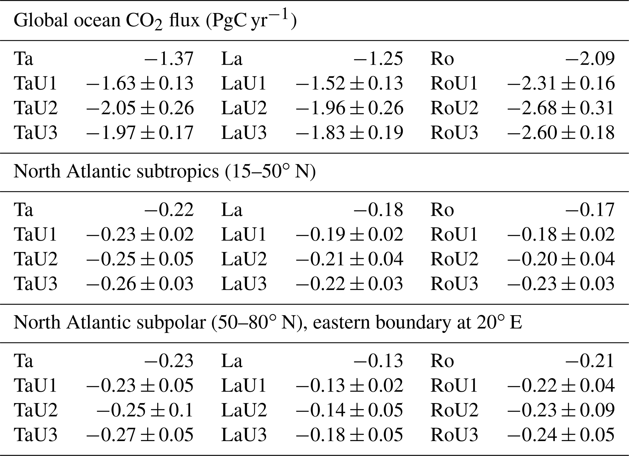
We note that the increases in estimated uptake for the North Atlantic basins are relatively smaller (on average in the range 10 %–20 %) than the increased uptake estimated on the global scale (∼ 30 %–50 % changes; see Table 1), indicating that the prior flux representations of North Atlantic carbon uptake are more consistent with the constraints from atmospheric CO2 measurements than the comparison on a global scale.
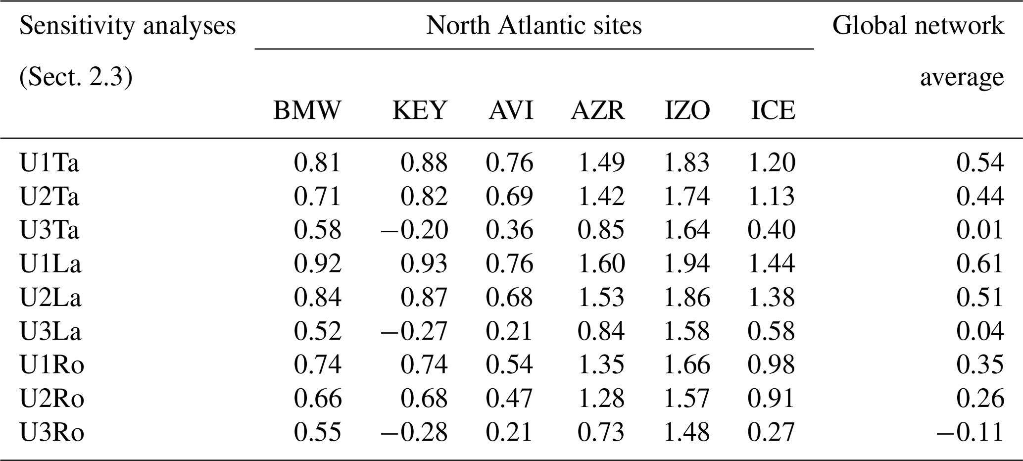
The U3 flux uncertainty specification is derived from the variation among a set of ocean–atmosphere carbon flux products (Eq. 1). This scheme specifies lower uncertainty levels where alternative prior flux representations are in accord (e.g., when well constrained by availability of surface pCO2 measurements, as in the subtropical North Atlantic) and higher uncertainty levels where the prior flux distributions differ significantly (typically in undersampled regions or those of significant flux variability, such as the subpolar North Atlantic). We further assess the value of the U3 scheme using a metric of GCL modeled atmospheric CO2 concentration; specifically, estimates of the model–observation mismatch for the year 2003 at the NOAA network station sites in the North Atlantic using the a posteriori fluxes associated with the sensitivity analyses of this section (Appendix Table A2). The results summarized in Table A2 indicate that scheme U3 provides the smallest-magnitude model–observation mismatch for the individual North Atlantic sites and for the global network average. Therefore, for the long-term analyses in the remainder of this study, we use the U3 spread-based flux uncertainty scheme in preference to the fixed-level flux uncertainty schemes used in many previous inverse analyses.
3.2 Multiyear analyses of North Atlantic CO2 fluxes
In this section we present results of a multiyear GCL analysis (for the period 2000–2017), calculating regional estimates of North Atlantic CO2 fluxes on annual to decadal timescales. Prior flux distributions for fossil fuel emissions and exchange with the land biosphere fluxes are as described in Sect. 2.4. For ocean prior fluxes, we employ the distribution of Landschützer et al. (2016); this is an established surface pCO2-based product and also provides interannually varying fluxes over the entire estimation period (2000–2017) in comparison to the climatology-only fluxes of Takahashi et al. (2009). Ocean prior flux uncertainties are specified by the spread-based scheme U3 described above and derived from the eight ocean–atmosphere pCO2-based flux products summarized in Sect. 2.4.

Figure 2Comparison of annual air–sea CO2 fluxes for North Atlantic for the 2000–2017 period for (a) North Atlantic subtropics and (b) North Atlantic subpolar regions. The GCL posterior flux estimate from this study (red) is derived from the prior flux of Landschützer et al. (2016) (pCO2La, black). The shaded grey area represents the uncertainty estimate on the GCL posterior flux (plotted at a 1σ level). Also shown are the flux estimates of (i) Chevallier et al. (2019) (CAMS, yellow), (ii) Jacobson et al. (2020) (CT, CarbonTracker 2019, pink), and (iii) van der Laan-Luijkx et al. (2017) (CTE, Carbon Tracker Europe, blue). All time series shown have a 12-month running mean filter applied.
Figure 2 presents the variation of air–sea CO2 flux for the North Atlantic subtropical and subpolar regions for the 2000–2017 period (represented as a 12-month running average). We also plot in Fig. 2 flux estimates from three other atmospheric inverse analysis studies including CAMS (v18r2, Chevallier et al., 2019), CT (CarbonTracker 2019; Jacobson et al., 2020) and CTE (Carbon Tracker Europe; van der Laan-Luijkx et al., 2017). All data are regridded to 2∘ latitude × 2.5∘ longitude to be consistent with the GCL model resolution.

Figure 3Comparison of CO2 ocean flux metrics for the 2000–2017 period for North Atlantic subtropics (a, c, e) and subpolar regions (b, d, f). Metrics shown are the long-term mean (a, b), interannual variability (IAV) (c, d), and long-term trend (e, f). The GCL estimates (red stars) are shown in comparison to other atmospheric inverse analyses (red symbols), surface ocean pCO2 products (blue), and global ocean biogeochemistry models (GOBMs, purple). Also shown are the estimated mean values from each subgroup of analyses (filled cross symbols) with their minimum to maximum range. Circled symbols in (e) and (f) indicate a statistically significant trend.
For the North Atlantic subtropical region, the GCL posterior flux magnitude is close to that of the ocean prior flux employed (Landschutzer et al., 2016), with differences of approximately 0.01 PgC yr−1 over the period. Variation among the other inverse flux estimates can reach up to 0.3 PgC yr−1 (e.g., between CT and CAMS in 2017), and these differences can be ascribed, in part, to the different underlying prior flux distributions used in the respective inverse analyses (see Sect. 3.2.2). For the North Atlantic subpolar region, the GCL posterior flux estimate deviates more from the prior flux estimate (e.g., showing differences of up to 0.04 PgC yr−1), especially for some years (2012–2017) of the analysis. The majority of flux estimates for the North Atlantic subpolar region are in closer accord (Fig. 2b) with differences of less than 0.2 PgC yr−1 (the CT estimate is an exception indicating variations of greater than 0.3 PgC yr−1 from the other estimates). A potential reason for the anomalous behavior of the CT estimate in the North Atlantic is the underlying prior flux uncertainties used in the analysis, which give a loose constraint on the prior ocean fluxes and allow the ocean fluxes to deviate far from the prior fluxes influenced by the atmospheric CO2 signals (Jacobson et al., 2020).
We also note that Peylin et al. (2013) have suggested that significant interannual variability in atmospheric inverse estimates is a potential indicator of “flux leakage”, where significant variability of terrestrial carbon fluxes in combination with sparse atmospheric sampling can result in misattribution of carbon flux estimates between land and ocean. To assess the significance of flux leakage in our GCL analyses, we have calculated estimates of the diagnostic recommended by Peylin et al. (2013) (i.e., the correlation between the annual total land and total ocean fluxes) for the Northern Hemisphere as a whole (Equator to 90∘ N) and also by latitudinal region. Estimates of this diagnostic are relatively low for our GCL analyses (values of 0.2 and 0.5 for the subpolar and subtropical regions, respectively), indicating low potential for flux leakage. As a point of comparison, Peylin et al. (2013) note that 6 out of 11 atmospheric inverse analyses in their model intercomparison reported correlation coefficients of greater than 0.5.
3.2.1 Long-term mean
Figure 3 provides a comparison of the following GCL flux estimates and associated characteristics for the North Atlantic subtropical and subpolar regions for the period 2000–2017: (i) the long-term mean of air–sea CO2 flux estimates (the underlying data are tabulated in Table 2); (ii) the estimated interannual variability (IAV) of fluxes (Table 3); and (iii) the long-term trends (Table 4). The IAV is calculated following methods of Rödenbeck et al. (2015) (i.e., derived from the standard deviation of the residuals of a 12-month running mean over the CO2 flux time series).
Table 2Summary metrics of GEOS-Chem–LETKF North Atlantic (NA) CO2 flux estimates and comparison with independent estimates (from atmospheric inverse analyses, surface pCO2 mappings, and global ocean biogeochemistry models (GOBMs)) for the period 2000–2017. Listed are estimates for the long-term mean. The metrics listed in this table are plotted in Fig. 3a and b.

∗ The uncertainty of the long-term mean estimate from the GCL (this study) is calculated as the standard deviation of the annual flux estimates over the 2000–2017 period.
We also present in Fig. 3 the equivalent estimates from other independent assessments, including (i) other atmospheric inverse analyses, (ii) surface ocean pCO2-based analyses, and (iii) analyses from global ocean biogeochemistry models (GOBMs). For the North Atlantic subtropical region, the long-term mean of the GCL posterior flux estimate is −0.255 ± 0.037 PgC yr−1 (Fig. 3a and Table 2). It lies in the range spanned by the other inverse analyses (−0.31 to −0.20 PgC yr−1, of slightly larger magnitude than CAMS but smaller than CT and CTE) and is in good agreement with the mean-value estimates from surface pCO2-based methods and GOBMs. For the North Atlantic subpolar region, the GCL estimate of the long-term mean uptake is −0.203 ± 0.037 PgC yr−1 (Table 2), which is close to the inverse estimate of the CAMS analysis and of smaller magnitude (by ∼ 0.1 PgC yr−1) than the inverse estimates of CT and CTE. The GCL estimate is consistent with the mean estimate from pCO2-based products and within the range of flux estimates from GOBMs (from −0.341 to −0.197 PgC yr−1).
3.2.2 Interannual variability
The interannual variability (IAV) of CO2 flux estimates derived from the GCL is 0.036 ± 0.006 PgC yr−1 for the North Atlantic subtropics and 0.034 ± 0.009 PgC yr−1 for the North Atlantic subpolar region (Fig. 3c and d, Table 3). The IAV estimates from the different inverse analyses for both the North Atlantic subtropics and subpolar regions display a larger range (0.032 to 0.084 and 0.023 to 0.114 PgC yr−1, respectively) than the ranges displayed by GOBMs (0.014 to 0.027 and 0.015 to 0.024 PgC yr−1, respectively) and pCO2-based fluxes (0.029 to 0.050 and 0.009 to 0.037 PgC yr−1, respectively). The larger range of IAV from atmospheric inverse analyses is influenced especially by high-magnitude IAV estimates from the CarbonTracker (CT) inverse analysis. Potential causes of the differences among atmospheric inversion between the GCL and CAMS IAV estimates and those of the CarbonTracker estimates are the different prior ocean fluxes employed by the inverse analyses, and the relative weighting assigned to the influence of atmospheric CO2 observations (Jacobson et al., 2020). The GCL and CAMS estimates use the prior flux of Landschützer et al. (2016), CTE uses the prior flux of Rodenbeck et al. (2014), and the CarbonTracker inversions use the prior flux of Jacobson et al. (2007).
Recent synthesis studies of global ocean carbon fluxes have noted that GOBMs underestimate the magnitude of IAV in comparison to estimates from pCO2-based mappings and inverse analyses (DeVries et al., 2019; Hauck et al., 2020). An important driver of IAV is the variability in biological carbon export; the lower variability observed in the GOBMs could result from opposing changes in biological vs. circulation impacts on carbon export, which potentially reduces the sensitivity of the GOBM air–sea carbon fluxes to climate variability (Landschutzer et al., 2013; DeVries et al., 2019).
Table 3Summary metrics of GEOS-Chem–LETKF North Atlantic (NA) CO2 flux estimates and comparison with independent estimates (from atmospheric inverse analyses, surface pCO2 mappings, and global ocean biogeochemistry models (GOBMs)) for the period 2000–2017. Listed are estimates for the interannual variability of the regional fluxes over the period. The metrics listed in this table are plotted in Fig. 3c and d.
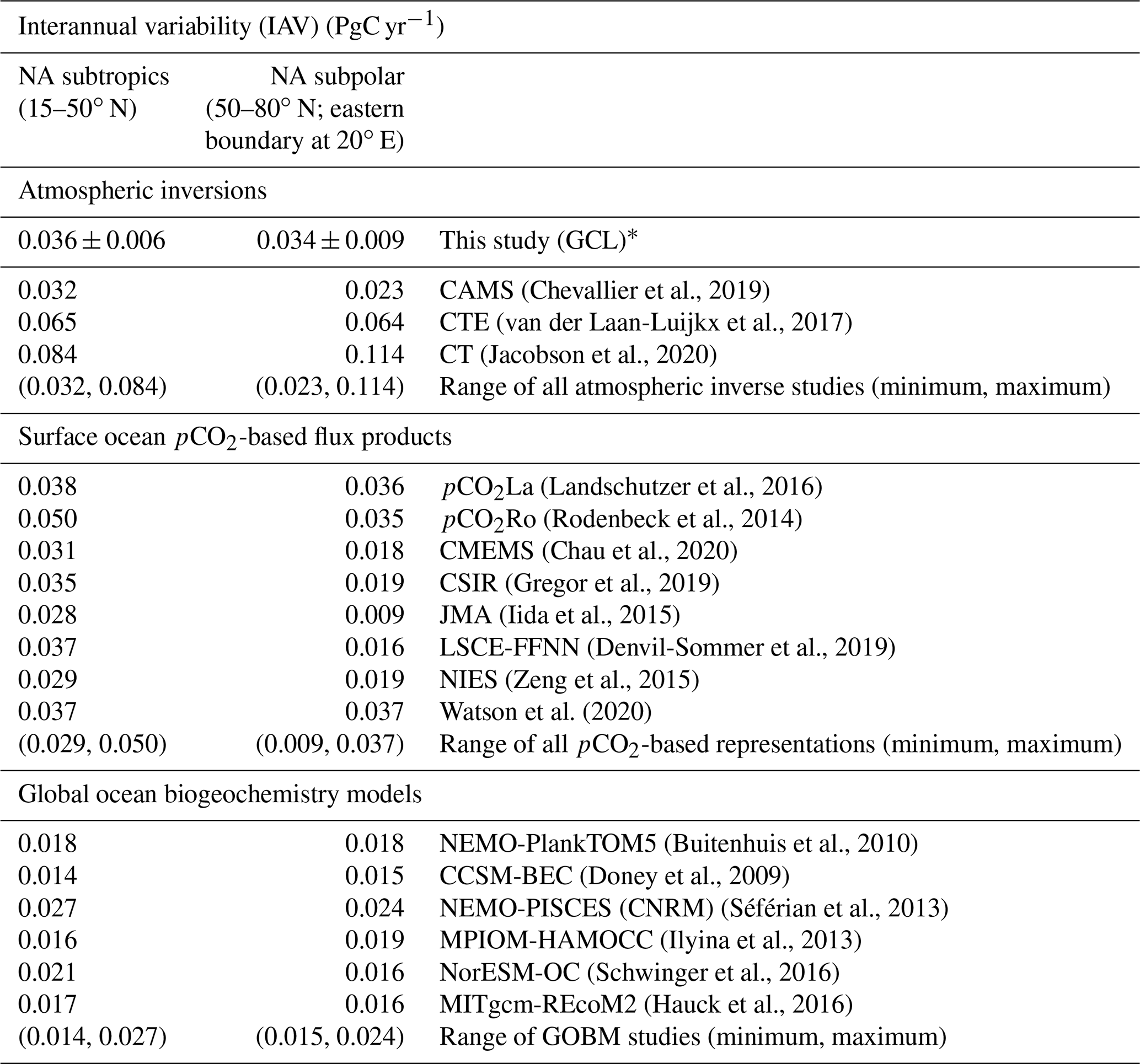
∗ The uncertainty of the estimated IAV from the GCL (this study) is calculated as the standard deviation of the ensemble posterior fluxes.
3.2.3 Estimated trends of North Atlantic CO2 fluxes
Our calculations of estimated trends for the 2000–2017 period are presented in Table 4 and Fig. 3e and f. We also highlight in the table and figure panels the trend estimates that are statistically significant (significant at the 95 % confidence level; Montgomery et al., 2012). Our GCL analyses indicate statistically significant trends for the 2000–2017 period of −0.064 ± 0.007 PgC yr−1 decade−1 in the North Atlantic subtropical basin and 0.063 ± 0.008 PgC yr−1 decade−1 in the subpolar region. These estimated trends are of similar magnitude to those estimated from surface ocean pCO2 products but of much larger magnitude (by a factor of 3–4) than decadal trends estimated from the GOBMs (Fig. 3e, Table 4). Our findings are similar to those of Devries et al. (2019), who noted that decadal trend estimates of North Atlantic CO2 uptake for the 2000s from the SOCOM (Surface Ocean pCO2 Mapping intercomparison) of pCO2-based flux products were larger than those from the GOBMs in their analysis (see Fig. 3 of their study).
Table 4Summary metrics of GEOS-Chem–LETKF North Atlantic (NA) CO2 flux estimates and comparison with independent estimates (from atmospheric inverse analyses, surface pCO2 mappings, and global ocean biogeochemistry models (GOBMs)) for the period 2000–2017. Listed are estimates for the trend of the regional fluxes over the period. The metrics listed in this table are plotted in Fig. 3e and f of the main study.

a The symbol “(S)” indicates that the calculated trend is statistically
significant (at the 95 % confidence interval).
b The uncertainty of the fitted trend from the GCL estimates is
reported as 1 standard deviation of the ordinary least squares (OLS)-fitted slope (Montgomery et al.,
2012).
In this study we present a new long-term estimate of North Atlantic air–sea CO2 fluxes for recent decades (period 2000–2017) using the atmospheric carbon cycle data assimilation system GEOS-Chem–LETKF. We focus, in particular, on the specification of prior ocean fluxes, including sensitivity of flux estimates to alternative prior flux distributions and on the specification of uncertainties associated with ocean fluxes. Towards this, we have developed the spread-based flux uncertainty scheme which represents the variability among a set of different prior ocean CO2 flux representations. The scheme ascribes higher levels of uncertainty to regions with larger discrepancies among ocean CO2 prior flux representation that arise from uncertainties associated with measurement density and pCO2-interpolation methods (Sect. 2.4). The spread-based flux uncertainty scheme provides improved performance in comparison to schemes with fixed prior flux uncertainty levels, based on an assessment metric of differences in model–observation values for atmospheric CO2 at North Atlantic measurement sites of the NOAA-GLOBALVIEWCO2 network (Sect. 3.1). It provides a valuable new means of specifying prior flux uncertainties for atmospheric inverse analyses of ocean CO2 fluxes.
We have used the spread-based flux uncertainty scheme in the GEOS-Chem–LETKF to derive estimates of CO2 fluxes in the North Atlantic for the 2000–2017 period. Long-term mean estimates of the regional ocean CO2 uptake are −0.255 ± 0.037 PgC yr−1 for the North Atlantic subtropics and −0.203 ± 0.037 PgC yr−1 for North Atlantic subpolar region, and they are consistent with recent regional flux estimates from surface pCO2-based methods and global ocean biogeochemistry models (GOBMs). The GEOS-Chem–LETKF estimates of interannual variability in air–sea CO2 fluxes are 0.036 ± 0.006 PgC yr−1 (North Atlantic subtropics) and 0.034 ± 0.009 PgC yr−1 (North Atlantic subpolar). In common with estimates from other atmospheric CO2 inverse studies, the magnitude of IAV derived from the GEOS-Chem–LETKF is larger than corresponding estimates from GOBMs. Our GEOS-Chem–LETKF estimates also indicate statistically significant trends of increasing CO2 uptake for the North Atlantic subtropical and subpolar regions (estimated trend of −0.064 ± 0.007 and −0.063 ± 0.008 PgC yr−1 decade−1, respectively). These trends are of comparable magnitude to those estimated from surface pCO2-based flux products, but much larger than those derived from global ocean biogeochemistry models for the 2000–2017 period. Estimates of interannual variability and long-term trends derived from our GEOS-Chem–LETKF analyses are generally more robust for the North Atlantic subtropics than for the subpolar region and characterized by smaller uncertainty bounds. Limiting factors affecting estimates for the North Atlantic subpolar region include higher levels of uncertainty associated with specification of prior fluxes (Fig. 1) and the observational uncertainty at the atmospheric measurement CO2 sites in these high northern latitudes (Table A1). The number of regional atmospheric CO2 measurement sites available to constrain North Atlantic subpolar fluxes are also relatively few in comparison to the subtropical region. Improved ocean CO2 flux estimates and associated metrics for this North Atlantic region will be obtained by provision of additional high accuracy marine boundary layer CO2 measurements for the region from fixed surface sites and from ships and buoys (Wanninkhof et al., 2019).
Here we briefly describe the LETKF system used for estimation of surface CO2 fluxes. The methodology follows that of Hunt et al. (2007) and Miyoshi et al. (2007), and additional detail is provided in these publications. The LETKF has been previously used in meteorological forecasting and more recently in atmospheric CO2 data assimilation (e.g., Liu et al., 2019, 2016; Kang et al., 2012). The LETKF provides iterative estimates of the time evolution of the system state, x, (here representing the grid-scale surface carbon fluxes of dimension m). Each step involves a forecast stage (based on a physical model of the system evolution) and a state estimation stage (the “analysis” step), which combines system observations, y (of dimension n), together with the background forecast, xb, to derive the improved state estimate. The observation operator H provides the mapping from the state space to the observation space; in this study H is provided by the GEOS-Chem atmospheric model. In the analysis step, the surface carbon flux estimates are obtained by minimization of a cost function (Eq. A1) which accounts for deviations of the system state x from the background forecast, xb, and for the mismatch between observations (y) and their modeled representations (Hx):
where B represents the background flux covariance matrix, and R represents the observation covariance matrix.
In the LETKF system, an ensemble of model simulations is used to calculate the sample mean and covariance of the system state; thus, the background state xb is given by ) for k ensemble members. The sample mean and covariance Pb of the background state vector are given by
where Xb is an m×k matrix whose ith column is . Pb is the background state covariance matrix (m×m).
Similarly the analysis state is represented by the ensemble ) with its sample mean and covariance given by
where Xa is the m×k matrix whose ith column is .
The analysis state and covariance, and Pa, are updated based on the background information and observations y through the following equations:
The ensemble yb(i) of background observation vectors is defined by
where Yb is the n×k matrix whose ith column is ), and w is a Gaussian random vector with mean and covariance . Then the analogues of analysis Eqs. (6) and (7) are
Following Hunt et al. (2007) and Miyoshi et al. (2007) (refer to these publications for the complete LETKF derivation) the overall analysis equation is
The LETKF allows for flexibility in the choice of observations to be assimilated at each grid point, based on the distance (r) of the observations from the grid point. The localization weighting function f(r) is given by
where L is an observation localization length which can be predefined to determine the outer boundary of the influence of the observations; i.e., the localization weighting function drops to zero at a value of
The observation localization is realized by multiplying the inverse of the localization function f(r) with the observational error covariance R.
The parameter L represents the horizontal localization radius and is set to 2000 km for this study, following Liu et al. (2016). The localization radius is used in the LETKF in a latitude-dependent weighting function which characterizes the spatial scale of the region within which atmospheric CO2 observations are assimilated at each grid point (Miyoshi et al., 2007).
Table A1Atmospheric CO2 measurement sitesa.
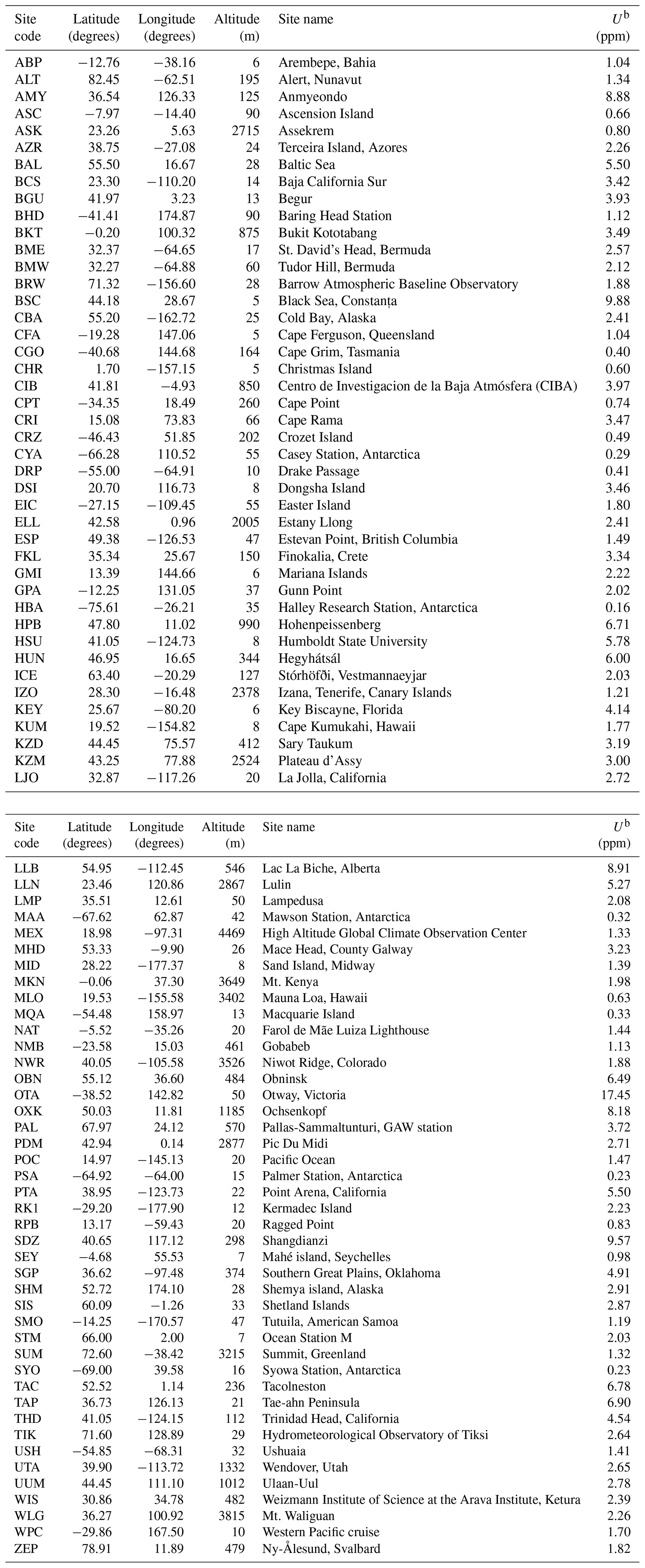
a Source reference: Cooperative Global Atmospheric Data Integration Project, 2018. Version: obspack_co2_1_GLOBALVIEWplus_v4.2_2019-03-19 (https://doi.org/10.25925/20190319, last access: 14 October 2020). b The specification of observational uncertainty U on atmospheric CO2 measurements (and represented in matrix R of Eq. A1) is calculated as the standard deviation of measurement variability and using the detrended and deseasonalized CO2 time series at each measurement site (following methods of Chevallier et al., 2010).
Table A2Model–observation mismatch in atmospheric CO2 concentrations (unit: ppm) at North Atlantic sites (average over year 2003). GCL model values are derived from the a posteriori model analyses associated with the sensitivity analyses of Sect. 3.1. Atmospheric CO2 observations are from the NOAA GLOBALVIEW network described in Sect. 2.3. Note AVI (−64.75∘, 17.76∘), site name: St. Croix, Virgin Islands. No observation is available during 2000–2017. Here the observations from the nearest site RPB (−59.43∘, 13.17∘) for 2003 are used.
The data sources are the following: (i) Atmospheric CO2 measurements were taken from obspack_co2_1_GLOBALVIEWplus_v4.2_2019-03-19 (https://gml.noaa.gov/ccgg/obspack/data.php?id=obspack_co2_1_GLOBALVIEWplus_v4.2_2019-03-19, (ObsPack, Cooperative Global Atmospheric Data Integration Project, 2018, last access: 14 October 2020); (ii) Prior ocean flux oc_v1.7 from Rödenbeck et al. (2013) were taken from http://www.bgc-jena.mpg.de/CarboScope/ (last access: 5 June 2020). Prior ocean flux from Landschützer et al. (2016) were taken from https://www.ncei.noaa.gov/access/ocean-carbon-data-system/oceans/SPCO2_1982_present_ETH_SOM_FFN.html (last access: 6 May 2020). Prior ocean flux from Takahashi et al. (2009) were taken from ftp://ftp.as.harvard.edu/gcgrid/geos-chem (last access: 9 July 2018). (iii) CarbonTracker CT2019 results were provided by NOAA ESRL, Boulder, Colorado, USA, from the website at http://carbontracker.noaa.gov (Jacobson et al., 2020, last access: 15 May 2020). CTE flux estimates were downloaded from ftp://ftp.wur.nl/carbontracker/data/fluxes/data_flux1x1_monthly/ (van der Laan-Luijkx et al., 2017, last access: 24 November 2020). The flux estimates from CAMS (v18r2) were taken from https://apps.ecmwf.int/datasets/data/cams-ghg-inversions/ (Chevallier et al., 2019, last access: 6 December 2019). (iv) The model CO2 fluxes for JULES (land) and GOBMs (ocean) were taken from Le Quéré et al. (2018). Time series of reconstructed surface ocean pCO2 and CO2 fluxes (LSCE-FFNN) from Denvil-Sommer et al. (2019) are the first version of CMEMS, downloaded from https://resources.marine.copernicus.eu/?option=com_csw&task=results (last access: 14 January 2021). The products from Iida et al. (2015) were downloaded from http://www.data.jma.go.jp/gmd/kaiyou/english/co2_flux/co2_flux_data_en.html (last access: 14 January 2021). The products from Zeng et al. (2015) were downloaded from https://db.cger.nies.go.jp/DL/10.17595/20201020.001.html.en (last access: 14 January 2021). The products from CMEMS, CSIR, and Watson were taken from Friedlingstein et al. (2020).
ZC and PS designed the study. ZC, PS, JZ, and NZ developed the model. ZC, PS, AJW, and US discussed the design of simulations. ZC performed the simulations and analysis and wrote the initial paper. All authors contributed to the writing of the paper.
The authors declare that they have no conflict of interest.
The work reflects only the author’s view; the European Commission and their executive agency are not responsible
for any use that may be made of the information the work contains.
Publisher’s note: Copernicus Publications remains neutral with regard to jurisdictional claims in published maps and institutional affiliations.
This work was performed using the High Performance Computing Cluster at the University of East Anglia.
This research has been supported by the Natural Environment Research Council (grant no. NE/K002473/1).
This paper was edited by Alexey V. Eliseev and reviewed by two anonymous referees.
Bakker, D. C. E., Pfeil, B., Landa, C. S., Metzl, N., O'Brien, K. M., Olsen, A., Smith, K., Cosca, C., Harasawa, S., Jones, S. D., Nakaoka, S., Nojiri, Y., Schuster, U., Steinhoff, T., Sweeney, C., Takahashi, T., Tilbrook, B., Wada, C., Wanninkhof, R., Alin, S. R., Balestrini, C. F., Barbero, L., Bates, N. R., Bianchi, A. A., Bonou, F., Boutin, J., Bozec, Y., Burger, E. F., Cai, W.-J., Castle, R. D., Chen, L., Chierici, M., Currie, K., Evans, W., Featherstone, C., Feely, R. A., Fransson, A., Goyet, C., Greenwood, N., Gregor, L., Hankin, S., Hardman-Mountford, N. J., Harlay, J., Hauck, J., Hoppema, M., Humphreys, M. P., Hunt, C. W., Huss, B., Ibánhez, J. S. P., Johannessen, T., Keeling, R., Kitidis, V., Körtzinger, A., Kozyr, A., Krasakopoulou, E., Kuwata, A., Landschützer, P., Lauvset, S. K., Lefèvre, N., Lo Monaco, C., Manke, A., Mathis, J. T., Merlivat, L., Millero, F. J., Monteiro, P. M. S., Munro, D. R., Murata, A., Newberger, T., Omar, A. M., Ono, T., Paterson, K., Pearce, D., Pierrot, D., Robbins, L. L., Saito, S., Salisbury, J., Schlitzer, R., Schneider, B., Schweitzer, R., Sieger, R., Skjelvan, I., Sullivan, K. F., Sutherland, S. C., Sutton, A. J., Tadokoro, K., Telszewski, M., Tuma, M., van Heuven, S. M. A. C., Vandemark, D., Ward, B., Watson, A. J., and Xu, S.: A multi-decade record of high-quality fCO2 data in version 3 of the Surface Ocean CO2 Atlas (SOCAT), Earth Syst. Sci. Data, 8, 383–413, https://doi.org/10.5194/essd-8-383-2016, 2016.
Bopp, L., Resplandy, L., Orr, J. C., Doney, S. C., Dunne, J. P., Gehlen, M., Halloran, P., Heinze, C., Ilyina, T., Séférian, R., Tjiputra, J., and Vichi, M.: Multiple stressors of ocean ecosystems in the 21st century: projections with CMIP5 models, Biogeosciences, 10, 6225–6245, https://doi.org/10.5194/bg-10-6225-2013, 2013.
Buitenhuis, E. T., Rivkin, R. B., Sailley, S., and Le Quéré, C.: Biogeochemical fluxes through microzooplankton, Glob. Biogeochem. Cy., 24, GB4015, https://doi.org/10.1029/2009GB003601, 2010.
Buitenhuis, E. T., Hashioka, T., and Le Quéré, C.: Combined constraints on global ocean primary production using observations and models, Global Biogeochem. Cy., 27, 847–858, https://doi.org/10.1002/gbc.20074, 2013.
Carouge, C., Bousquet, P., Peylin, P., Rayner, P. J., and Ciais, P.: What can we learn from European continuous atmospheric CO2 measurements to quantify regional fluxes – Part 1: Potential of the 2001 network, Atmos. Chem. Phys., 10, 3107–3117, https://doi.org/10.5194/acp-10-3107-2010, 2010.
Chatterjee, A., Engelen, R. J., Kawa, S. R., Sweeney, C., and Michalak, A. M.: Background error covariance estimation for atmospheric CO2 data assimilation, J. Geophys. Res.-Atmos., 118, 10140–10154, https://doi.org/10.1002/jgrd.50564, 2013.
Chau, T. T., Gehlen, M., and Chevallier, F.: Global Ocean Surface Carbon Product MULTIOBS_textunderscore GLO_BIO_CARBON_SURFACE_REP_015_008, E.U. Copernicus Marine Service Information, available at: https://resources.marine.copernicus.eu/?option=com_cswandview=detailsandproduct_id=MULTIOBS_G, last access: 16 November 2020.
Chevallier, F., Ciais, P., Conway, T., Aalto, T., Anderson, B., Bousquet, P., Brunke, E., Ciattaglia, L., Esaki, Y., and Fröhlich, M.: CO2 surface fluxes at grid point scale estimated from a global 21 year reanalysis of atmospheric measurements, J. Geophys. Res.-Atmos., 115, D21307, https://doi.org/10.1029/2010JD013887, 2010.
Chevallier, F., Palmer, P. I., Feng, L., Boesch, H., O'Dell, C. W., and Bousquet, P.: Toward robust and consistent regional CO2 flux estimates from in situ and spaceborne measurements of atmospheric CO2, Geophys. Res. Lett., 41, 1065–1070, https://doi.org/10.1002/2013GL058772, 2014.
Chevallier, F., Remaud, M., O'Dell, C. W., Baker, D., Peylin, P., and Cozic, A.: Objective evaluation of surface- and satellite-driven carbon dioxide atmospheric inversions [data set], Atmos. Chem. Phys., 19, 14233–14251, https://doi.org/10.5194/acp-19-14233-2019, 2019.
Clark, D. B., Mercado, L. M., Sitch, S., Jones, C. D., Gedney, N., Best, M. J., Pryor, M., Rooney, G. G., Essery, R. L. H., Blyth, E., Boucher, O., Harding, R. J., Huntingford, C., and Cox, P. M.: The Joint UK Land Environment Simulator (JULES), model description – Part 2: Carbon fluxes and vegetation dynamics, Geosci. Model Dev., 4, 701–722, https://doi.org/10.5194/gmd-4-701-2011, 2011.
Crippa, M., Janssens-Maenhout, G., Dentener, F., Guizzardi, D., Sindelarova, K., Muntean, M., Van Dingenen, R., and Granier, C.: Forty years of improvements in European air quality: regional policy-industry interactions with global impacts, Atmos. Chem. Phys., 16, 3825–3841, https://doi.org/10.5194/acp-16-3825-2016, 2016.
Denvil-Sommer, A., Gehlen, M., Vrac, M., and Mejia, C.: LSCE-FFNN-v1: a two-step neural network model for the reconstruction of surface ocean pCO2 over the global ocean [data set], Geosci. Model Dev., 12, 2091–2105, https://doi.org/10.5194/gmd-12-2091-2019, 2019.
DeVries, T., Le Quéré, C., Andrews, O., Berthet, S., Hauck, J., Ilyina, T., Landschützer, P., Lenton, A., Lima, I. D., and Nowicki, M.: Decadal trends in the ocean carbon sink, P. Natl. Acad. Sci. USA, 116, 11646–11651, https://doi.org/10.1073/pnas.1900371116, 2019.
Doney, S. C., Lima, I., Feely, R. A., Glover, D. M., Lindsay, K., Mahowald, N., Moore, J. K., and Wanninkhof, R.: Mechanisms governing interannual variability in upper-ocean inorganic carbon system and air–sea CO2 fluxes: Physical climate and atmospheric dust, Deep Sea Res. Pt. II, 56, 640–655, https://doi.org/10.1016/j.dsr2.2008.12.006, 2009.
Feng, L., Palmer, P. I., Parker, R. J., Deutscher, N. M., Feist, D. G., Kivi, R., Morino, I., and Sussmann, R.: Estimates of European uptake of CO2 inferred from GOSAT X retrievals: sensitivity to measurement bias inside and outside Europe, Atmos. Chem. Phys., 16, 1289–1302, https://doi.org/10.5194/acp-16-1289-2016, 2016.
Friedlingstein, P., O'Sullivan, M., Jones, M. W., Andrew, R. M., Hauck, J., Olsen, A., Peters, G. P., Peters, W., Pongratz, J., Sitch, S., Le Quéré, C., Canadell, J. G., Ciais, P., Jackson, R. B., Alin, S., Aragão, L. E. O. C., Arneth, A., Arora, V., Bates, N. R., Becker, M., Benoit-Cattin, A., Bittig, H. C., Bopp, L., Bultan, S., Chandra, N., Chevallier, F., Chini, L. P., Evans, W., Florentie, L., Forster, P. M., Gasser, T., Gehlen, M., Gilfillan, D., Gkritzalis, T., Gregor, L., Gruber, N., Harris, I., Hartung, K., Haverd, V., Houghton, R. A., Ilyina, T., Jain, A. K., Joetzjer, E., Kadono, K., Kato, E., Kitidis, V., Korsbakken, J. I., Landschützer, P., Lefèvre, N., Lenton, A., Lienert, S., Liu, Z., Lombardozzi, D., Marland, G., Metzl, N., Munro, D. R., Nabel, J. E. M. S., Nakaoka, S.-I., Niwa, Y., O'Brien, K., Ono, T., Palmer, P. I., Pierrot, D., Poulter, B., Resplandy, L., Robertson, E., Rödenbeck, C., Schwinger, J., Séférian, R., Skjelvan, I., Smith, A. J. P., Sutton, A. J., Tanhua, T., Tans, P. P., Tian, H., Tilbrook, B., van der Werf, G., Vuichard, N., Walker, A. P., Wanninkhof, R., Watson, A. J., Willis, D., Wiltshire, A. J., Yuan, W., Yue, X., and Zaehle, S.: Global Carbon Budget 2020, Earth Syst. Sci. Data, 12, 3269–3340, https://doi.org/10.5194/essd-12-3269-2020, 2020.
Gaubert, B., Stephens, B. B., Basu, S., Chevallier, F., Deng, F., Kort, E. A., Patra, P. K., Peters, W., Rödenbeck, C., Saeki, T., Schimel, D., Van der Laan-Luijkx, I., Wofsy, S., and Yin, Y.: Global atmospheric CO2 inverse models converging on neutral tropical land exchange, but disagreeing on fossil fuel and atmospheric growth rate, Biogeosciences, 16, 117–134, https://doi.org/10.5194/bg-16-117-2019, 2019.
Gregor, L., Lebehot, A. D., Kok, S., and Scheel Monteiro, P. M.: A comparative assessment of the uncertainties of global surface ocean CO2 estimates using a machine-learning ensemble (CSIR-ML6 version 2019a) – have we hit the wall?, Geosci. Model Dev., 12, 5113–5136, https://doi.org/10.5194/gmd-12-5113-2019, 2019.
Gruber, N., Gloor, M., Mikaloff Fletcher, S. E., Doney, S. C., Dutkiewicz, S., Follows, M. J., Gerber, M., Jacobson, A. R., Joos, F., and Lindsay, K.: Oceanic sources, sinks, and transport of atmospheric CO2, Glob. Biogeochem. Cy., 23, GB1005, https://doi.org/10.1029/2008GB003349, 2009.
Gruber, N., Landschützer, P., and Lovenduski, N. S.: The variable Southern Ocean carbon sink, Annu. Rev. Mar. Sci., 11, 159–186, https://doi.org/10.1146/annurev-marine-121916-063407, 2019.
Gurney, K. R., Law, R., Denning, A. S., Rayner, P. J., Baker, D., Bousquet, P., Bruhwiler, L., Chen, Y. H., Ciais, P., Fan, S., Fung, I. Y., Gloor, M., Heimann, M., Higuchi, K., John, J., Maki, T., Maksyutov, S., Masarie, K., Peylin, P., Prather, M., Pak, B. C., Randerson, J., Sarmiento, J., Taguchi, S., Takahashi, T., and Yuan, C.: Towards robust regional estimates of CO2 sources and sinks using atmospheric transport models, Nature, 415, 626–630, https://doi.org/10.1038/415626a, 2002.
Gurney, K. R., Law, R. M., Denning, A. S., Rayner, P. J., Baker, D., Bousquet, P., Bruhwiler, L., Chen, Y. H., Ciais, P., and Fan, S.: TransCom 3 CO2 inversion intercomparison: 1. Annual mean control results and sensitivity to transport and prior flux information, Tellus B, 55, 555–579, https://doi.org/10.3402/tellusb.v55i2.16728, 2003.
Hauck, J., Köhler, P., Wolf-Gladrow, D., and Völker, C.: Iron fertilisation and century-scale effects of open ocean dissolution of olivine in a simulated CO2 removal experiment, Environ. Res. Lett., 11, 024007, https://doi.org/10.1088/1748-9326/11/2/024007, 2016.
Hauck, J., Zeising, M., Le Quéré, C., Gruber, N., Bakker, D. C., Bopp, L., Chau, T. T., Gürses, Ö., Ilyina, T., Landschützer, P., Lenton, A., Resplandy, L., Rödenbeck, C., Schwinger, J., and Séférian, R.: Consistency and challenges in the ocean carbon sink estimate for the Global Carbon Budget, Front. Mar. Sci., 7, 852, https://doi.org/10.3389/fmars.2020.571720, 2020.
Hunt, B. R., Kostelich, E. J., and Szunyogh, I.: Efficient data assimilation for spatiotemporal chaos: A local ensemble transform Kalman filter, Physica D, 230, 112–126, https://doi.org/10.1016/j.physd.2006.11.008, 2007.
Iida, Y., Kojima, A., Takatani, Y., Nakano, T. Midorikawa, T., and Ishii, M.: Trends in pCO2 and sea-air CO2 flux over the global open oceans for the last two decades [data set], J. Oceanogr., 71, 637–661, https://doi.org/10.1007/s10872-015-0306-4, 2015.
Ilyina, T., Six, K. D., Segschneider, J., Maier-Reimer, E., Li, H., and Núñez-Riboni, I.: Global ocean biogeochemistry model HAMOCC: Model architecture and performance as component of the MPI-Earth system model in different CMIP5 experimental realizations, J. Adv. Model. Earth Sys., 5, 287–315, https://doi.org/10.1029/2012MS000178, 2013.
Jacobson, A. R., Mikaloff Fletcher, S. E., Gruber, N., Sarmiento, J. L., and Gloor, M.: A joint atmosphere-ocean inversion for surface fluxes of carbon dioxide: 1. Methods and global-scale fluxes, Glob. Biogeochem. Cy., 21, GB1019, https://doi.org/10.1029/2005GB002556, 2007.
Jacobson, A. R., Schuldt, K. N., Miller, J. B., Oda, T., Tans, P., Andrews, A., Mund, J., Ott, L., Collatz, G. J., Aalto, T., Afshar, S., Aikin, K., Aoki, S., Apadula, F., Baier, B., Bergamaschi, P., Beyersdorf, A., Biraud, S. C., Bollenbacher, A., Bowling, D., Brailsford, G., Abshire, J. B., Chen, G., Chen, H., Chmura, L., Climadat, S., Colomb, A., Conil, S., Cox, A., Cristofanelli, P., Cuevas, E., Curcoll, R., Sloop, C. D., Davis, K., Wekker, S. D., Delmotte, M., DiGangi, J. P., Dlugokencky, E., Ehleringer, J., Elkins, J. W., Emmenegger, L., Fischer, M. L., Forster, G., Frumau, A., Galkowski, M., Gatti, L. V., Gloor, E., Griffis, T., Hammer, S., Haszpra, L., Hatakka, J., Heliasz, M., Hensen, A., Hermanssen, O., Hintsa, E., Holst, J., Jaffe, D., Karion, A., Kawa, S. R., Keeling, R., Keronen, P., Kolari, P., Kominkova, K., Kort, E., Krummel, P., Kubistin, D., Labuschagne, C., Langenfelds, R., Laurent, O., Laurila, T., Lauvaux, T., Law, B., Lee, J., Lehner, I., Leuenberger, M., Levin, I., Levula, J., Lin, J., Lindauer, M., Loh, Z., Lopez, M., Lund Myhre, C., Machida, T., Mammarella, I., Manca, G., Manning, A., Manning, A., Marek, M. V., Marklund, P., Martin, M. Y., Matsueda, H., McKain, K., Meijer, H., Meinhardt, F., Miles, N., Miller, C. E., Mölder, M., Montzka, S., Moore, F., Morgui, J., Morimoto, S., Munger, B., Necki, J., Newman, S., Nichol, S., Niwa, Y., O'Doherty, S., Ottosson-Löfvenius, M., Paplawsky, B., Peischl, J., Peltola, O., Pichon, J., Piper, S., Plass-Dölmer, C., Ramonet, M., Reyes-Sanchez, E., Richardson, S., Riris, H., Ryerson, T., Saito, K., Sargent, M., Sasakawa, M., Sawa, Y., Say, D., Scheeren, B., Schmidt, M., Schmidt, A., Schumacher, M., Shepson, P., Shook, M., Stanley, K., Steinbacher, M., Stephens, B., Sweeney, C., Thoning, K., Torn, M., Turnbull, J., Tørseth, K., van den Bulk, P., van der Laan-Luijkx, I. T., van Dinther, D., Vermeulen, A., Viner, B., Vitkova, G., Walker, S., Weyrauch, D., Wofsy, S., Worthy, D., Young, D., and Zimnoch, M.: CarbonTracker CT2019, Model published by NOAA Earth System Research Laboratory, Global Monitoring Division [data set], available at: https://gml.noaa.gov/ccgg/carbontracker/CT2019B_doc.php, last access: 15 October 2020.
Jones, S. D., Le Quéré, C., and Rödenbeck, C.: Autocorrelation characteristics of surface ocean pCO2 and air-sea CO2 fluxes, Global Biogeochem. Cy., 26, 2, https://doi.org/10.1029/2010GB004017, 2012.
Kang, J. S., Kalnay, E., Liu, J., Fung, I., Miyoshi, T., and Ide, K.: “Variable localization” in an ensemble Kalman filter: Application to the carbon cycle data assimilation, J. Geophys. Res.-Atmos., 116, D09110, https://doi.org/10.1029/2010JD014673, 2011.
Kang, J. S., Kalnay, E., Miyoshi, T., Liu, J., and Fung, I.: Estimation of surface carbon fluxes with an advanced data assimilation methodology, J. Geophys. Res.-Atmos., 117, D24101, https://doi.org/10.1029/2012JD018259, 2012.
Khatiwala, S., Tanhua, T., Mikaloff Fletcher, S., Gerber, M., Doney, S. C., Graven, H. D., Gruber, N., McKinley, G. A., Murata, A., Ríos, A. F., and Sabine, C. L.: Global ocean storage of anthropogenic carbon, Biogeosciences, 10, 2169–2191, https://doi.org/10.5194/bg-10-2169-2013, 2013.
Landschützer, P., Gruber, N., Bakker, D. C., Schuster, U., Nakaoka, S. I., Payne, M. R., Sasse, T. P., and Zeng, J.: A neural network-based estimate of the seasonal to inter-annual variability of the Atlantic Ocean carbon sink, Biogeosciences, 10, 7793–7815, https://doi.org/10.5194/bg-10-7793-2013, 2013.
Landschuetzer, P., Gruber, N., and Bakker, D. C.: Decadal variations and trends of the global ocean carbon sink [data set], Global Biogeochem. Cy., 30, 1396–1417, https://doi.org/10.1002/2015GB005359, 2016.
Landschützer, P., Ilyina, T., and Lovenduski, N. S.: Detecting Regional Modes of Variability in Observation-Based Surface Ocean pCO2, Geophys. Res. Lett., 46, 2670–2679, https://doi.org/10.1029/2018GL081756, 2019.
Le Quéré, C., Andrew, R. M., Friedlingstein, P., Sitch, S., Pongratz, J., Manning, A. C., Korsbakken, J. I., Peters, G. P., Canadell, J. G., Jackson, R. B., Boden, T. A., Tans, P. P., Andrews, O. D., Arora, V. K., Bakker, D. C. E., Barbero, L., Becker, M., Betts, R. A., Bopp, L., Chevallier, F., Chini, L. P., Ciais, P., Cosca, C. E., Cross, J., Currie, K., Gasser, T., Harris, I., Hauck, J., Haverd, V., Houghton, R. A., Hunt, C. W., Hurtt, G., Ilyina, T., Jain, A. K., Kato, E., Kautz, M., Keeling, R. F., Klein Goldewijk, K., Körtzinger, A., Landschützer, P., Lefèvre, N., Lenton, A., Lienert, S., Lima, I., Lombardozzi, D., Metzl, N., Millero, F., Monteiro, P. M. S., Munro, D. R., Nabel, J. E. M. S., Nakaoka, S., Nojiri, Y., Padin, X. A., Peregon, A., Pfeil, B., Pierrot, D., Poulter, B., Rehder, G., Reimer, J., Rödenbeck, C., Schwinger, J., Séférian, R., Skjelvan, I., Stocker, B. D., Tian, H., Tilbrook, B., Tubiello, F. N., van der Laan-Luijkx, I. T., van der Werf, G. R., van Heuven, S., Viovy, N., Vuichard, N., Walker, A. P., Watson, A. J., Wiltshire, A. J., Zaehle, S., and Zhu, D.: Global Carbon Budget 2017, Earth Syst. Sci. Data, 10, 405–448, https://doi.org/10.5194/essd-10-405-2018, 2018.
Lebehot, A. D., Halloran, P. R., Watson, A. J., McNeall, D., Ford, D. A., Landschützer, P., Lauvset, S. K., and Schuster, U.: Reconciling observation and model trends in North Atlantic surface CO2, Global Biogeochem. Cy., 33, 1204–1222, https://doi.org/10.1029/2019GB006186, 2019.
Liu, J., Bowman, K. W., and Lee, M.: Comparison between the Local Ensemble Transform Kalman Filter (LETKF) and 4D-Var in atmospheric CO2 flux inversion with the Goddard Earth Observing System-Chem model and the observation impact diagnostics from the LETKF, J. Geophys. Res.-Atmos., 121, 13066–13087, https://doi.org/10.1002/2016JD025100, 2016.
Liu, Y., Kalnay, E., Zeng, N., Asrar, G., Chen, Z., and Jia, B.: Estimating surface carbon fluxes based on a local ensemble transform Kalman filter with a short assimilation window and a long observation window: an observing system simulation experiment test in GEOS-Chem 10.1, Geosci. Model Dev., 12, 2899–2914, https://doi.org/10.5194/gmd-12-2899-2019, 2019.
Macovei, V. A., Hartman, S. E., Schuster, U., Torres-Valdés, S., Moore, C. M., and Sanders, R. J.: Impact of physical and biological processes on temporal variations of the ocean carbon sink in the mid-latitude North Atlantic (2002–2016), Prog. Oceanogr., 180, 102223, https://doi.org/10.1016/j.pocean.2019.102223, 2020.
McKinley, G. A., Fay, A. R., Takahashi, T., and Metzl, N.: Convergence of atmospheric and North Atlantic carbon dioxide trends on multidecadal timescales, Nat. Geosci., 4, 606–610, https://doi.org/10.1038/ngeo1193, 2011.
Mikaloff Fletcher, S., Gruber, N., Jacobson, A. R., Doney, S., Dutkiewicz, S., Gerber, M., Follows, M., Joos, F., Lindsay, K., and Menemenlis, D.: Inverse estimates of anthropogenic CO2 uptake, transport, and storage by the ocean, Global Biogeochem. Cy., 20, GB2002, https://doi.org/10.1029/2005GB002530, 2006.
Miyoshi, T., Yamane, S., and Enomoto, T.: Localizing the error covariance by physical distances within a local ensemble transform Kalman filter (LETKF), SOLA, 3, 89–92, https://doi.org/10.2151/sola.2007-023, 2007.
Montgomery, D. C., Peck, E. A., and Vining, G. G.: Introduction to Linear Regression Analysis,5th Edition, John Wiley & Sons, 645 pp., 2012.
Nassar, R., Jones, D. B. A., Suntharalingam, P., Chen, J. M., Andres, R. J., Wecht, K. J., Yantosca, R. M., Kulawik, S. S., Bowman, K. W., Worden, J. R., Machida, T., and Matsueda, H.: Modeling global atmospheric CO2 with improved emission inventories and CO2 production from the oxidation of other carbon species, Geosci. Model Dev., 3, 689–716, https://doi.org/10.5194/gmd-3-689-2010, 2010.
Nassar, R., Jones, D. B. A., Kulawik, S. S., Worden, J. R., Bowman, K. W., Andres, R. J., Suntharalingam, P., Chen, J. M., Brenninkmeijer, C. A. M., Schuck, T. J., Conway, T. J., and Worthy, D. E.: Inverse modeling of CO2 sources and sinks using satellite observations of CO2 from TES and surface flask measurements, Atmos. Chem. Phys., 11, 6029–6047, https://doi.org/10.5194/acp-11-6029-2011, 2011.
Peters, W., Miller, J., Whitaker, J., Denning, A., Hirsch, A., Krol, M., Zupanski, D., Bruhwiler, L., and Tans, P.: An ensemble data assimilation system to estimate CO2 surface fluxes from atmospheric trace gas observations, J. Geophys. Res.-Atmos., 110, D24304, https://doi.org/10.1029/2005JD006157, 2005.
Peylin, P., Law, R. M., Gurney, K. R., Chevallier, F., Jacobson, A. R., Maki, T., Niwa, Y., Patra, P. K., Peters, W., Rayner, P. J., Rödenbeck, C., van der Laan-Luijkx, I. T., and Zhang, X.: Global atmospheric carbon budget: results from an ensemble of atmospheric CO2 inversions, Biogeosciences, 10, 6699–6720, https://doi.org/10.5194/bg-10-6699-2013, 2013.
Rienecker, M. M., Suarez, M., Todling, R., Bacmeister, J., Takacs, L., Liu, H., Gu, W., Sienkiewicz, M., Koster, R., and Gelaro, R.: The GEOS-5 Data Assimilation System: Documentation of Versions 5.0.1, 5.1.0, and 5.2.0, NASA Technical Report Series on Global Modelling and Data Assimilation,NASA/TM–2008–104606, 27, 2008.
Rödenbeck, C., Houweling, S., Gloor, M., and Heimann, M.: Time-dependent atmospheric CO2 inversions based on interannually varying tracer transport, Tellus B, 55, 488–497, https://doi.org/10.3402/tellusb.v55i2.16707, 2003.
Rödenbeck, C., Keeling, R. F., Bakker, D. C. E., Metzl, N., Olsen, A., Sabine, C., and Heimann, M.: Global surface-ocean pCO2 and sea–air CO2 flux variability from an observation-driven ocean mixed-layer scheme [data set], Ocean Sci., 9, 193–216, https://doi.org/10.5194/os-9-193-2013, 2013.
Rödenbeck, C., Bakker, D. C. E., Metzl, N., Olsen, A., Sabine, C., Cassar, N., Reum, F., Keeling, R. F., and Heimann, M.: Interannual sea–air CO2 flux variability from an observation-driven ocean mixed-layer scheme, Biogeosciences, 11, 4599–4613, https://doi.org/10.5194/bg-11-4599-2014, 2014.
Rödenbeck, C., Bakker, D. C. E., Gruber, N., Iida, Y., Jacobson, A. R., Jones, S., Landschützer, P., Metzl, N., Nakaoka, S., Olsen, A., Park, G.-H., Peylin, P., Rodgers, K. B., Sasse, T. P., Schuster, U., Shutler, J. D., Valsala, V., Wanninkhof, R., and Zeng, J.: Data-based estimates of the ocean carbon sink variability – first results of the Surface Ocean pCO2 Mapping intercomparison (SOCOM), Biogeosciences, 12, 7251–7278, https://doi.org/10.5194/bg-12-7251-2015, 2015.
Sabine, C. L., Feely, R. A., Gruber, N., Key, R. M., Lee, K., Bullister, J. L., Wanninkhof, R., Wong, C., Wallace, D. W., and Tilbrook, B.: The oceanic sink for anthropogenic CO2, Science, 305, 367–371, https://doi.org/10.1126/science.1097403, 2004.
Schuster, U., McKinley, G. A., Bates, N., Chevallier, F., Doney, S. C., Fay, A., González-Dávila, M., Gruber, N., Jones, S., and Krijnen, J.: An assessment of the Atlantic and Arctic sea-air CO2 fluxes, 1990–2009, Biogeosciences, 10, 607–627, https://doi.org/10.5194/bg-10-607-2013, 2013.
Schwinger, J., Goris, N., Tjiputra, J. F., Kriest, I., Bentsen, M., Bethke, I., Ilicak, M., Assmann, K. M., and Heinze, C.: Evaluation of NorESM-OC (versions 1 and 1.2), the ocean carbon-cycle stand-alone configuration of the Norwegian Earth System Model (NorESM1), Geosci. Model Dev., 9, 2589–2622, https://doi.org/10.5194/gmd-9-2589-2016, 2016.
Séférian, R., Bopp, L., Gehlen, M., Orr, J. C., Ethé, C., Cadule, P., Aumont, O., Mélia, D. S., Voldoire, A., and Madec, G.: Skill assessment of three earth system models with common marine biogeochemistry, Clim. Dynam., 40, 2549–2573, https://doi.org/10.1007/s00382-012-1362-8, 2013.
Suntharalingam, P., Randerson, J. T., Krakauer, N., Logan, J. A., and Jacob, D. J.: Influence of reduced carbon emissions and oxidation on the distribution of atmospheric CO2: Implications for inversion analyses, Global Biogeochem. Cy., 19, GB4003, https://doi.org/10.1029/2005GB002466, 2005.
Takahashi, T., Sutherland, S. C., Sweeney, C., Poisson, A., Metzl, N., Tilbrook, B., Bates, N., Wanninkhof, R., Feely, R. A., and Sabine, C.: Global sea–air CO2 flux based on climatological surface ocean pCO2, and seasonal biological and temperature effects, Deep Sea Res. Pt. II, 49, 1601–1622, https://doi.org/10.1016/S0967-0645(02)00003-6, 2002.
Takahashi, T., Sutherland, S. C., Wanninkhof, R., Sweeney, C., Feely, R. A., Chipman, D. W., Hales, B., Friederich, G., Chavez, F., and Sabine, C.: Climatological mean and decadal change in surface ocean pCO2, and net sea–air CO2 flux over the global oceans [data set], Deep Sea Res. Pt. II, 56, 554–577, https://doi.org/10.1016/j.dsr2.2008.12.009, 2009.
van der Laan-Luijkx, I. T., van der Velde, I. R., van der Veen, E., Tsuruta, A., Stanislawska, K., Babenhauserheide, A., Zhang, H. F., Liu, Y., He, W., Chen, H., Masarie, K. A., Krol, M. C., and Peters, W.: The CarbonTracker Data Assimilation Shell (CTDAS) v1.0: implementation and global carbon balance 2001–2015 [data set], Geosci. Model Dev., 10, 2785–2800, https://doi.org/10.5194/gmd-10-2785-2017, 2017.
Wanninkhof, R., Pickers, P., Omar, A., Sutton, A., Murata, A., Olsen, A., Bb, S., Tilbrook, B., Munro, D., and Pierrot, D.: A surface ocean CO2 reference network, SOCONET and associated marine boundary layer CO2 measurements, Front. Mar. Sci., 6, 400, https://doi.org/10.3389/fmars.2019.00400, 2019.
Watson, A. J., Schuster, U., Bakker, D. C., Bates, N. R., Corbière, A., González-Dávila, M., Friedrich, T., Hauck, J., Heinze, C., and Johannessen, T.: Tracking the variable North Atlantic sink for atmospheric CO2, Science, 326, 1391–1393, https://doi.org/10.1126/science.1177394, 2009.
Watson, A. J., Schuster, U., Shutler, J. D., Holding, T., Ashton, I. G. C., Landschützer, P., Woolf, D. K., and Goddijn-Murphy, L.: Revised estimates of ocean-atmosphere CO2 flux are consistent with ocean carbon inventory, Nat. Commun., 11, 1–6, https://doi.org/10.1038/s41467-020-18203-3, 2020.
Zeng, J., Nojiri, Y., Nakaoka, Shin-ichiro, Nakajima, H., and Shirai, T.: Surface ocean CO2 in 1990–2011 modelled using a feed-forward neural network [data set], Geosci. Data J., 2, 47–51, https://doi.org/10.1002/gdj3.26, 2015.
Ziehn, T., Lenton, A., Law, R. M., Matear, R. J., and Chamberlain, M. A.: The carbon cycle in the Australian Community Climate and Earth System Simulator (ACCESS-ESM1) – Part 2: Historical simulations, Geosci. Model Dev., 10, 2591–2614, https://doi.org/10.5194/gmd-10-2591-2017, 2017.