Derivation of seawater pCO₂ from net community production identifies the South Atlantic Ocean as a CO₂ source

A key step in assessing the global carbon budget is the determination of the partial pressure of CO₂ in seawater (pCO_2 (sw)). Spatially complete observational fields of pCO_2 (sw) are routinely produced for regional and global ocean carbon budget assessments by extrapolating sparse in situ measurements of pCO_2 (sw) using satellite observations. As part of this process, satellite chlorophyll a (Chl a) is often used as a proxy for the biological drawdown or release of CO₂. Chl a does not, however, quantify carbon fixed through photosynthesis and then respired, which is determined by net community production (NCP).

In this study, pCO_2 (sw) over the South Atlantic Ocean is estimated using a feed forward neural network (FNN) scheme and either satellite-derived NCP, net primary production (NPP) or Chl a to compare which biological proxy produces the most accurate fields of pCO_2 (sw). Estimates of pCO_2 (sw) using NCP, NPP or Chl a were similar, but NCP was more accurate for the Amazon Plume and upwelling regions, which were not fully reproduced when using Chl a or NPP. A perturbation analysis assessed the potential maximum reduction in pCO_2 (sw) uncertainties that could be achieved by reducing the uncertainties in the satellite biological parameters. This illustrated further improvement using NCP compared to NPP or Chl a. Using NCP to estimate pCO_2 (sw) showed that the South Atlantic Ocean is a CO₂ source, whereas if no biological parameters are used in the FNN (following existing annual carbon assessments), this region appears to be a sink for CO₂. These results highlight that using NCP improved the accuracy of estimating pCO_2 (sw) and changes the South Atlantic Ocean from a CO₂ sink to a source. Reducing the uncertainties in NCP derived from satellite parameters will ultimately improve our understanding and confidence in quantification of the global ocean as a CO₂ sink.

1 Introduction

Since the industrial revolution, anthropogenic CO₂ emissions have resulted in an increase in atmospheric CO₂ concentrations (Friedlingstein et al., 2020; IPCC, 2013). By acting as a sink for CO₂, the oceans have buffered the increase in anthropogenic atmospheric CO₂, without which the atmospheric concentration would be 42 %–44 % higher (DeVries, 2014). The long-term absorption of CO₂ by the oceans is altering the marine carbonate chemistry of the ocean, resulting in a lowering of pH, a process known as ocean acidification (Raven et al., 2005). Observational fields of the partial pressure of CO₂ in seawater (pCO_2 (sw)) are one of the key datasets needed to routinely assess the strength of the oceanic CO₂ sink (Friedlingstein et al., 2020; Landschützer et al., 2014, 2020; Rödenbeck et al., 2015; Watson et al., 2020b). These methods are reliant on the extrapolation of sparse in situ observations of pCO_2 (sw) using satellite observations of parameters which account for the variability of, and the controls on, pCO_2 (sw) (Shutler et al., 2020). These parameters include sea surface temperature (SST; e.g. Landschützer et al., 2013; Stephens et al., 1995), salinity and chlorophyll a (Chl a) (Rödenbeck et al., 2015). SST and salinity control pCO_2 (sw) by changing the solubility of CO₂ in seawater (Weiss, 1974), whilst biological processes such as photosynthesis and respiration contribute by modulating its concentration.

Chl a is routinely used as a proxy for the biological activity (Rödenbeck et al., 2015), but it does not distinguish between carbon fixation through photosynthesis and the carbon respired by the plankton community. Net primary production (the net carbon fixation rate; NPP) is determined by the standing stock of phytoplankton, for which the Chl a concentration is used as a proxy, and modified by the photosynthetic rate and the available light in the water column (Behrenfeld et al., 2016). Photosynthetic rates are, in turn, modified by ambient nutrient and temperature conditions (Behrenfeld and Falkowski, 1997; Marañón et al., 2003). Elevated Chl a does not always equate to elevated NPP (Poulton et al., 2006), and for the same Chl a concentrations, NPP can vary depending on the health and metabolic state of the plankton community. All of these controls are captured by the net community production (NCP), which is the metabolic balance of the plankton community resulting from the carbon fixed through photosynthesis and that lost through respiration. Where NCP is positive, the plankton community is autotrophic, which implies that there is a drawdown of CO₂ from seawater (since the plankton reduce the CO₂ in the water column). Where NCP is negative, the community is heterotrophic, implying a release of CO₂ into the ocean (as the plankton produce or release CO₂), which can then be released into the atmosphere (Jiang et al., 2019; Schloss et al., 2007). Using NCP to estimate pCO_2 (sw) compared to Chl a should theoretically lead to an improvement in the derivation of pCO_2 (sw).

Many studies have used satellite Chl a to estimate pCO_2 (sw) at both regional (Benallal et al., 2017; Chierici et al., 2012; Moussa et al., 2016) and global scales (Landschützer et al., 2014; Liu and Xie, 2017). Chierici et al. (2012) attempted to use satellite NPP to estimate pCO_2 (sw) in the southern Pacific Ocean, but there was no significant improvement over using satellite Chl a. This is not surprising as NPP captures more of the biological signal but still lacks any inclusion of respiration, which results in the release of CO₂ into the water column. To our knowledge the use of satellite NCP to estimate pCO_2 (sw) has not been attempted before and could be a means of improving estimates of pCO_2 (sw) as long as satellite NCP observations are accurate (Ford et al., 2021b; Tilstone et al., 2015). These satellite measurements may improve the estimation of pCO_2 (sw) as NCP includes the full biological control on pCO_2 (sw). This is particularly important in regions where in situ pCO_2 (sw) observations are sparse and where interpolation and neural network techniques are therefore likely to struggle (Watson et al., 2020b).

The South Atlantic Ocean is undersampled with limited pCO_2 (sw) observations (e.g. Fay and McKinley, 2013; Watson et al., 2020b). The region is varied and dynamic as it includes the seasonal equatorial upwelling, high biological activity on the south-western (Dogliotti et al., 2014) and south-eastern shelves (Lamont et al., 2014), and the propagation of the Amazon Plume into the western equatorial Atlantic (Ibánhez et al., 2015). This dynamic biogeochemical variability in conjunction with a comprehensive database of satellite observation-based data with associated uncertainties (Ford et al., 2021b) provides the potential to identify the improvement to pCO_2 (sw) estimates that could be made from using NCP.

The objective of this paper is to compare the estimation of pCO_2 (sw) using either NCP, NPP or Chl a to determine which biological descriptor produces the most accurate and complete pCO_2 (sw) fields. A 16-year time series of pCO_2 (sw) was generated for the South Atlantic Ocean using satellite NCP, NPP or Chl a, as the biological input, alongside two approaches with no biological input parameters. Regional differences in the resulting pCO_2 (sw) fields are assessed. The seasonal and interannual variabilities in pCO_2 (sw) estimated from NCP, NPP, Chl a and the approaches with no biological parameters were also compared. A perturbation analysis was conducted to evaluate the potential reduction in the uncertainty in the pCO_2 (sw) fields when estimated from NCP, NPP or Chl a. This is discussed in the context of reducing uncertainties in these input variables for future improvements in spatially complete fields of pCO_2 (sw) and the effect on estimates of the oceanic carbon sink.

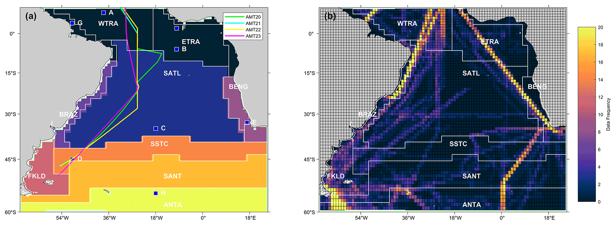
Figure 1 (a) Map of the eight static biogeochemical provinces in the South Atlantic Ocean, following Longhurst et al. (1995) and Longhurst (1998). Markers and letters indicate the locations of time series extracted from Fig. 3. The four Atlantic Meridional Transect (AMT) cruise tracks are also overlaid. (b) Map showing the spatial distribution of the SOCATv2020 data set used, where the data frequency is the number of available months of data within each 1^∘ pixel. The province areas acronyms are listed as follows: WTRA is western tropical Atlantic; ETRA is eastern equatorial Atlantic; SATL is South Atlantic Gyre; BRAZ is Brazilian current coastal; BENG is Benguela Current coastal upwelling; FKLD is Southwest Atlantic shelves; SSTC is South Subtropical Convergence; SANT is sub-Antarctic and ANTA is Antarctic.

2 Methods

2.1 Surface Ocean CO₂ Atlas (SOCAT) pCO_2 (sw) and atmospheric CO₂

SOCATv2020 (Bakker et al., 2016; Pfeil et al., 2013) individual fugacity of CO₂ in seawater (fCO_2 (sw)) observations were downloaded from https://www.socat.info/index.php/data-access/, last access: 17 June 2020. Data were extracted from 2002 to 2018 for the South Atlantic Ocean (10^∘ N–60^∘ S, 25^∘ E–80^∘ W; Fig. 1b). The individual cruise observations were collected from different depths and are not representative of the fCO_2 (sw) in the top ∼ 100 µm of the ocean, where gas exchange occurs (Goddijn-Murphy et al., 2015; Woolf et al., 2016). Therefore, the SOCAT observations were reanalysed to a standard temperature data set and depth (Reynolds et al., 2002) that is considered representative of the bottom of the mass boundary layer (Woolf et al., 2016). This was achieved using the “fe_reanalyse_socat” utility in the open-source FluxEngine toolbox (Holding et al., 2019; Shutler et al., 2016), which follows the methodology described in Goddijn-Murphy et al. (2015). The reanalysed fCO_2 (sw) observations were converted to pCO_2 (sw) and gridded onto 1^∘ monthly grids following SOCAT protocols (Sabine et al., 2013). The uncertainties in the in situ data were taken as the standard deviation of the observations in each grid cell or where a single observation exists were set as 5 µatm following Bakker et al. (2016).

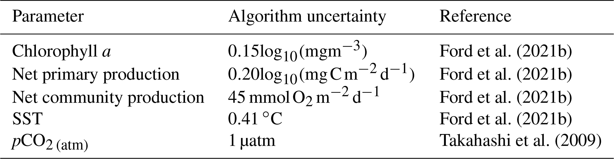
Table 1 Uncertainties in the input parameters of the feed forward neural network used in Monte Carlo uncertainty propagation and perturbation analysis.

Monthly 1^∘ grids of atmospheric pCO₂ (pCO_2 (atm)) were extracted from v5.5 of the global estimates of pCO_2 (sw) data set (Landschützer et al., 2016, 2017). pCO_2 (atm) was estimated using the dry mixing ratio of CO₂ from the NOAA-ESRL marine boundary layer reference (https://www.esrl.noaa.gov/gmd/ccgg/mbl/, last access: 25 September 2020), Optimum Interpolated SST (Reynolds et al., 2002) and sea level pressure following Dickson et al. (2007).

2.2 Moderate Resolution Imaging Spectroradiometer on Aqua (MODIS-A) satellite observations

The 4 km resolution monthly mean Chl a was calculated from MODIS-A level-1 granules, retrieved from National Aeronautics and Space Administration (NASA) Ocean Color website (https://oceancolor.gsfc.nasa.gov/, last access: 10 December 2020) using SeaDAS v7.5 and applying the standard OC3-CI Chl a algorithm (https://oceancolor.gsfc.nasa.gov/atbd/chlor_a/, last access: 15 December 2020). In addition, monthly mean MODIS-A SST and photosynthetically active radiation (PAR) were also downloaded from the NASA Ocean Color website. Mean monthly NPP were generated from MODIS-A Chl a, SST and PAR using the wavelength resolving model (Morel, 1991) with the lookup table described in Smyth et al. (2005). Coincident mean monthly NCP values using the algorithm NCP-D described in Tilstone et al. (2015) were generated using the MODIS-A NPP and SST data. Further details of the satellite algorithms are given in O'Reilly et al. (1998), O'Reilly and Werdell (2019), and Hu et al. (2012) for Chl a, Smyth et al. (2005) and Tilstone et al. (2005, 2009) for NPP, and Tilstone et al. (2015) for NCP. These satellite algorithms were shown to be the most accurate for the South Atlantic Ocean in an algorithm inter-comparison, which accounted for the uncertainties in both in situ, model and input data (Ford et al., 2021b). All monthly mean data were generated between July 2002 and December 2018 and were re-gridded onto the same 1^∘ grid as the pCO_2 (sw) observations. The assessed uncertainties from the literature for each of the input parameters used are given in Table 1.

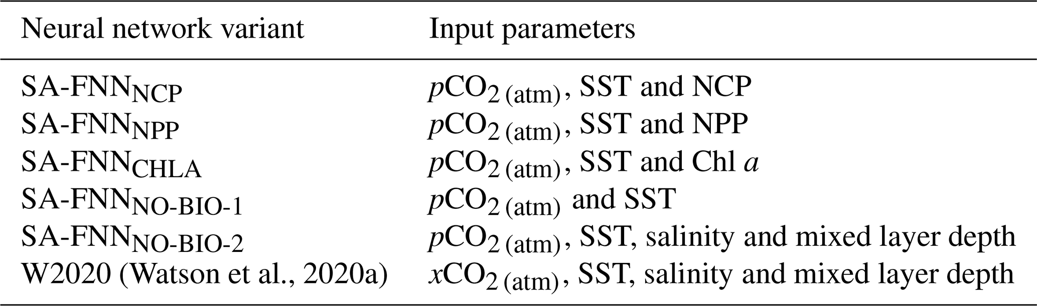
Table 2 The input parameters of the neural network variants described in Sects. 2.3. and 2.6. xCO₂ is the atmospheric mixing ratio of CO₂.

2.3 Feed forward neural network scheme

The South Atlantic Ocean was partitioned into eight biogeochemical provinces (Fig. 1a), following Longhurst et al. (1995) and Longhurst (1998). The pCO_2 (sw) observations in the eastern equatorial Atlantic were sparse, and therefore the equatorial region was merged into one province. In each province the available monthly pCO_2 (sw) observations were matched to temporally and spatially coincident pCO_2 (atm), MODIS-A, NCP and SST to provide training data for the feed forward neural network (FNN). Observations in coastal regions (< 200 m water depth) were removed from the analysis, due to the increased uncertainty in ocean colour observations in these areas (e.g. Lavender et al., 2004). Due to constraints on the coverage of ocean colour data, no data were available in austral winter below ∼ 50^∘ S.

The coincident observations in each province were randomly split into three datasets: (1) a training data set (50 % of the observations) used to train the FNNs; (2) a validation data set (30 % of the observations) used to assess the performance of the FNN and to prevent the networks from overfitting; and (3) an independent test data set (20 % of the observations) to assess the final performance of the FNN, with observations that are independent of the network training. The optimal split (r_opt) method of Amari et al. (1997) was used to partition the input data into these three sets, as follows:

$$\begin{array}{}\text{(1)}& r_{\text{opt}}=\mathrm{1}-{\displaystyle \frac{\mathrm{1}}{\sqrt{\mathrm{2}m}}},\end{array}$$

where m is number of input parameters. For our three input parameters, an optimal split of 60 % training data to 40 % validation data would occur, where we removed 10 % from each data set to provide a further independent test data set. A pre-training step was used to determine the optimum number of hidden neurons in the FNN (Benallal et al., 2017; Landschützer et al., 2013; Moussa et al., 2016) to provide the best fit for the observations, whilst preventing overfitting (Demuth et al., 2008).

The FNNs consist of one hidden layer with between 2 and 30 nodes depending on the pre-training step and one output layer. The networks were trained using the optimum number of hidden neurons, in an iterative process until the root mean square difference (RMSD) remained unchanged for six iterations. The best-performing FNN, with the lowest RMSD, was then used to estimate pCO_2 (sw). The uncertainties in the input parameters were propagated through the FNN, using a Monte Carlo uncertainty propagation, where 1000 calculations were made perturbing the input parameters, using random noise for their uncertainty (Table 1). The output from the eight province FNNs was then combined, and weighted statistics, which account for both the satellite and in situ uncertainty, were used to assess the overall performance of the FNN (as also used in Ford et al., 2021b). The combined eight-FNN approach will hereafter be referred to as SA-FNN.

The approach to training the FNNs was repeated replacing NCP with Chl a or NPP sequentially (Table 2) to determine if there was an improvement by using NCP. Chl a and NPP estimates were log ₁₀-transformed before input into the FNN, due to their respective uncertainties being determined in log ₁₀ space (Table 1). A baseline SA-FNN with no biological parameters as input was trained using pCO_2 (atm) and MODIS-A SST (SA-FNN_NO-BIO-1; Table 2). A second SA-FNN with no biological parameters (SA-FNN_NO-BIO-2; Table 2) was trained with the addition of sea surface salinity and mixed layer depth from the Copernicus Marine Environment Modelling Service (https://resources.marine.copernicus.eu/, last access: 20 August 2020) global ocean physics reanalysis product (GLORYS12V1). This parameter combination (pCO_2 (atm), SST, salinity and mixed layer depth) has recently been included within a neural network scheme to estimate global fields of pCO_2 (sw) (Watson et al., 2020b).

Following these methods, a monthly mean time series of pCO_2 (sw) was generated in the South Atlantic Ocean, applying the SA-FNN approach using NCP (SA-FNN_NCP), NPP (SA-FNN_NPP), Chl a (SA-FNN_CHLA) or no biological parameters (SA-FNN_NO-BIO-1 and SA-FNN_NO-BIO-2). The pCO_2 (sw) fields were spatially averaged using a 3 pixel × 3 pixel filter but were not averaged temporally as in previous studies (Landschützer et al., 2014, 2016) because averaging temporally could mask features that occur within single months of the year. The uncertainties in the input parameters (Table 1) were propagated through the neural network on a per-pixel basis and combined in quadrature with the RMSD of the test data set to produce a combined uncertainty budget for each pixel, assuming all sources of uncertainty are independent and uncorrelated (BIPM, 2008; Taylor, 1997).

2.4 Atlantic Meridional Transect in situ data

To assess the accuracy of the SA-FNN, coincident in situ measurements of NCP, NPP, Chl a, SST, pCO_2 (atm) and pCO_2 (sw), with uncertainties, were provided by Atlantic Meridional Transects 20, 21, 22 and 23 in 2010, 2011, 2012 and 2013, respectively. All the Atlantic Meridional Transect data described in this section can be obtained from the British Oceanographic Data Centre (https://www.bodc.ac.uk/, last access: 11 April 2020). Chl a was computed following the methods of Brewin et al. (2016), using underway continuous spectrophotometric measurements from AMT 22, and uncertainties were estimated as ∼ 0.06 log ₁₀(mg m⁻³) (Ford et al., 2021b). ¹⁴C-based NPP measurements were made based on dawn-to-dusk simulated in situ incubations, following the methods given in Tilstone et al. (2017), at 56 stations with a per-station uncertainty. Uncertainties ranged between 8 and 213 $\mathrm{mg}\mathrm{C}{\mathrm{m}}^{-\mathrm{2}}{\mathrm{d}}^{-\mathrm{1}}$ and were on average 53 $\mathrm{mg}\mathrm{C}{\mathrm{m}}^{-\mathrm{2}}{\mathrm{d}}^{-\mathrm{1}}$. NCP was estimated using in vitro changes in dissolved O₂, following the methods of Gist et al. (2009) and Tilstone et al. (2015) at 51 stations with a per-station uncertainty calculated. Uncertainties ranged between 5 and 25 $\mathrm{mmol}{\mathrm{O}}_{\mathrm{2}}{\mathrm{m}}^{-\mathrm{2}}{\mathrm{d}}^{-\mathrm{1}}$ and were on average 14 $\mathrm{mmol}{\mathrm{O}}_{\mathrm{2}}{\mathrm{m}}^{-\mathrm{2}}{\mathrm{d}}^{-\mathrm{1}}$.

Underway measurements of pCO_2 (sw) and pCO_2 (atm) were performed continuously, following the methods of Kitidis et al. (2017). SST was continuously measured alongside all observations (Sea-Bird SBE45), with a factory-calibrated uncertainty of ± 0.01 ^∘C. The mean of underway pCO_2 (sw), pCO_2 (atm), SST and Chl a were taken ± 20 min around each station where NCP and NPP were measured. These pCO_2 (sw) observations (N≈ 200) were removed from the SOCATv2020 data set so that the Atlantic Meridional Transect data remained independent from the training and validation datasets.

2.5 Perturbation analysis

Following the approach of Saba et al. (2011), a perturbation analysis was conducted to evaluate the potential reduction in SA-FNN pCO_2 (sw) RMSD that could be attributed to the input parameters. The analysis indicates the maximum reduction in RMSD that could be achieved if uncertainties in the input parameters were reduced to ∼ 0. Each of the input parameters – NCP, SST and pCO_2 (atm) – can have three possible values for each in situ pCO_2 (sw) observation (original value, original ± uncertainty; Table 1), enabling 27 perturbations of the input data as input to the SA-FNN. For each in situ pCO_2 (sw) observation, the 27 perturbations of SA-FNN pCO_2 (sw) were examined, and the perturbation that produced the lowest RMSD and bias combination was selected. The RMSD and bias were calculated between all the in situ pCO_2 (sw) and the selected perturbations. The percentage difference between this RMSD and the original RMSD when training the SA-FNN was calculated to indicate the maximum achievable reduction. This approach was conducted for two scenarios: (1) uncertainty in individual input parameters (NCP, SST and pCO_2 (atm)) and (2) uncertainty in all input parameters together. The approach was conducted on all three training datasets and on the Atlantic Meridional Transect in situ data. The analysis was repeated sequentially replacing NCP with Chl a and NPP to determine if there was a greater maximum reduction in RMSD using NCP. The analysis was also conducted allowing for a 10 % reduction in input parameter uncertainties to indicate the short-term reduction in pCO_2 (sw) RMSD that could be achieved by reducing the input parameter uncertainties.

2.6 Comparison of the SA-FNN_NCP with the SA-FNN_NO-BIO, SA-FNN_CHLA, SA-FNN_NPP and state-of-the-art data for the South Atlantic

The most comprehensive pCO_2 (sw) fields to date are from Watson et al. (2020a, b). The “standard method” pCO_2 (sw) fields within the Watson et al. (2020a, b) data were produced by extrapolating the in situ reanalysed SOCATv2019 pCO_2 (sw) observations using a self-organising-map feed forward neural network approach (Landschützer et al., 2016), hereafter referred to as “W2020”. A time series was extracted from the W2020 data, coincident with SA-FNN_NCP, SA-FNN_NPP, SA-FNN_CHLA and the two SA-FNN_NO-BIO variants. For the six methods, a monthly climatology referenced to the year 2010 was computed, assuming an atmospheric CO₂ increase of 1.5 µatm yr⁻¹ (Takahashi et al., 2009; Zeng et al., 2014). The climatology should be insensitive to the assumed rise in atmospheric CO₂ due to the reference year being central to the time series. The standard deviation of this climatology was also computed on a per-pixel basis.

The stations (Fig. 1) are representative of locations from previous literature that analysed the variability of in situ pCO_2 (sw) in the South Atlantic Ocean. For each station, the monthly climatology of pCO_2 (sw), representing the average seasonal cycle of pCO_2 (sw), and the standard deviation of the climatology, as an indication of the interannual variability, were extracted from the six approaches. The pCO_2 (sw) value for each station was the statistical mean of the four nearest data points weighted by their respective proximity to the station coordinate. In situ pCO_2 (sw) observations from the SOCATv2020 Flag E data set were also extracted for stations A and B (Fig. 1a), and a climatology was generated. These observations represent data from the Prediction and Research Moored Array in the Atlantic (PIRATA) buoys at these locations (Bourlès et al., 2008).

The station climatologies for the SA-FNN_NO-BIO-1, SA-FNN_NO-BIO-2, W2020, SA-FNN_CHLA and SA-FNN_NPP were compared to the SA-FNN_NCP, by testing for significant differences in the seasonal cycle and annual pCO_2 (sw) (offset). The seasonal cycles (seasonality) were compared using a non-parametric Spearman correlation and deemed statistically different where the correlation was not significant (α < 0.05). A non-parametric Kruskal–Wallis test was used to test for significant (α < 0.05) differences in the annual pCO_2 (sw), indicating an offset between the two tested climatologies. The Southern Ocean station (station H) was excluded from the statistical analysis due to missing data in the SA-FNN.

2.7 Estimation of the bulk CO₂ flux

The flux of CO₂ (F) between the atmosphere and ocean (air–sea) can be expressed in a bulk parameterisation as

$$\begin{array}{}\text{(2)}& F=k({\mathit{\alpha }}_{\mathrm{w}}\mathit{\text{p}}{\mathrm{CO}}_{\mathrm{2}\left(\mathrm{sw}\right)}-{\mathit{\alpha }}_{\mathrm{s}}\mathit{\text{p}}{\mathrm{CO}}_{\mathrm{2}\left(\mathrm{atm}\right)}),\end{array}$$

where k is the gas transfer velocity, and α_w and α_s are the solubility of CO₂ at the base and top of the mass boundary layer at the sea surface, respectively (Woolf et al., 2016). k was estimated from ERA5 monthly reanalysis wind speed (downloaded from the Copernicus Climate Data Store; https://cds.climate.copernicus.eu/, last access: 12 March 2020) following the parameterisation of Nightingale et al. (2000). The parameter α_w was estimated as a function of SST and sea surface salinity (Weiss, 1974) using the monthly Optimum Interpolated SST (Reynolds et al., 2002) and sea surface salinity from the Copernicus Marine Environment Modelling Service global ocean physics reanalysis product (GLORYS12V1). The α_s parameter was estimated using the same temperature and salinity datasets but included a gradient from the base to the top of mass boundary layer of −0.17 K (Donlon et al., 1999) and +0.1 salinity units (Woolf et al., 2016). pCO_2 (atm) was estimated using the dry mixing ratio of CO₂ from the NOAA-ESRL marine boundary layer reference, Optimum Interpolated SST (Reynolds et al., 2002) applying a cool skin bias (0.17 K; Donlon et al., 1999) and sea level pressure following Dickson et al. (2007). Spatially and temporally complete pCO_2 (sw) fields, which are representative of pCO_2 (sw) at the base of the mass boundary layer, were extracted from the SA-FNN_NCP, SA-FNN_NPP, SA-FNN_CHLA, SA-FNN_NO-BIO-1, SA-FNN_NO-BIO-2 and W2020.

The monthly CO₂ flux was calculated using the open-source FluxEngine toolbox (Holding et al., 2019; Shutler et al., 2016) between 2003 and 2018 for the six pCO_2 (sw) inputs, using the “rapid transport” approximation (described in Woolf et al., 2016). The net annual flux was determined for the South Atlantic Ocean (10^∘ N–44^∘ S, 25^∘ E–70^∘ W) using the “fe_calc_budgets.py” utility within FluxEngine with the supplied area and land percentage masks. The mean net annual flux was calculated as the mean of the 15-year net annual fluxes. Positive net fluxes indicate a net source to the atmosphere, and negative net fluxes represent a sink.

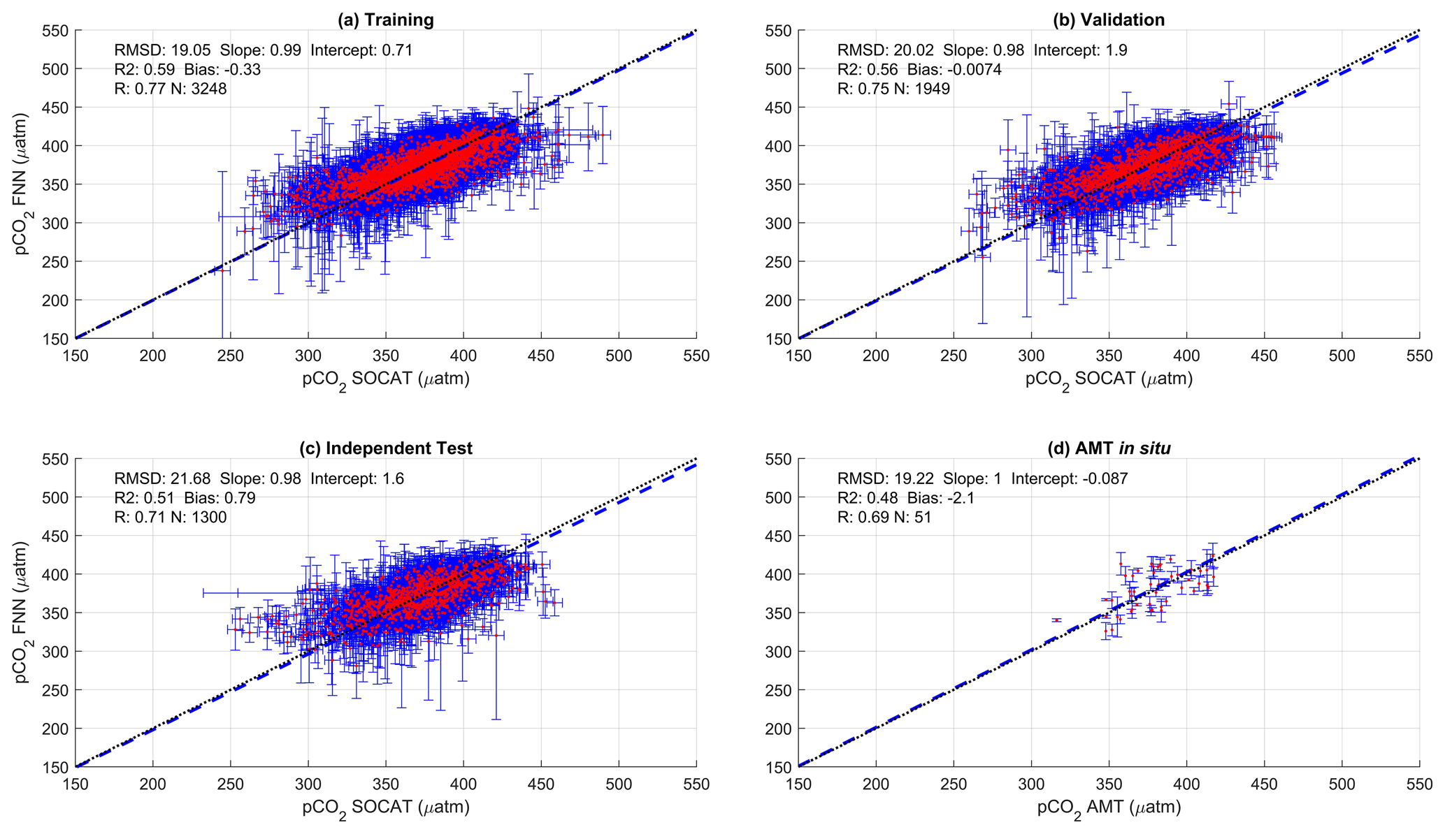
Figure 2 Scatter plots showing the combined performance of the eight feed forward neural networks trained using NCP for each biogeochemical province (Fig. 1) using four separate training and validation datasets: (a) training, (b) validation, (c) independent test and (d) Atlantic Meridional Transect (AMT) in situ. The data points are highlighted in red to distinguish them from the error bars in blue. The blue dashed line is the type II regression, and the black dashed line is the 1:1 line. Horizontal error bars indicate the uncertainty of the SOCATv2020 pCO_2 (sw). Vertical error bars indicate the uncertainty attributed to the input parameter uncertainty propagated through the feed forward neural networks. The statistics within each plot are the root mean square difference (RMSD), slope and intercept of the type II regression, coefficient of determination (R²), Pearson correlation coefficient (R), bias and number of samples (N).

3 Results

3.1 SA-FNN performance and perturbation analysis

The performance of the SA-FNN trained using pCO_2 (atm), SST and NCP for the three training datasets is given in Fig. 2. The SA-FNN_NCP had an accuracy (RMSD) of 21.68 µatm and a precision (bias) of 0.87 µatm, which was determined with the independent test data (N=1300). Training the SA-FNN using Chl a or NPP instead of NCP resulted in a similar performance (Appendix A Figs. A1 and A2). The RMSD for the independent test data was within ∼ 1.5 µatm for Chl a (19.88 µatm), NPP (20.48 µatm) and NCP (21.68 µatm), and bias was near zero.

Table 3 The percentage reduction in pCO_2 (sw) RMSD by reducing NCP, NPP and Chl a uncertainties to ∼ 0 as described in Sect. 2.5. The full results can be found in Appendix Table A1.

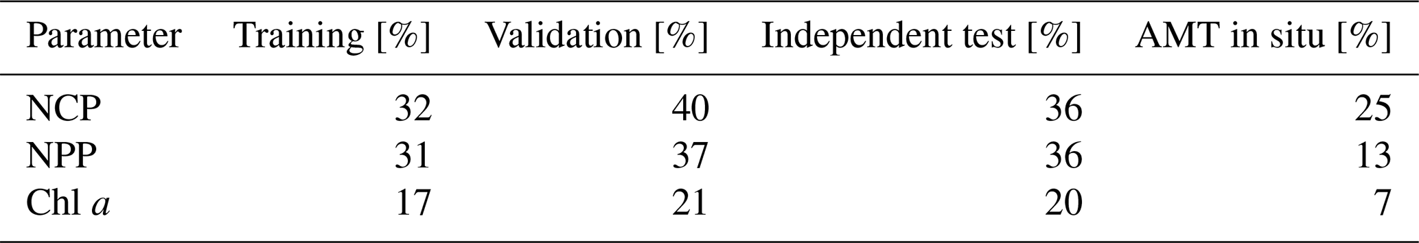
The reduction in pCO_2 (sw) RMSD that could be achieved if input parameter uncertainties were reduced to ∼ 0 was assessed using the perturbation analysis (Table 3, Appendix A Table A1). This showed that a reduction in pCO_2 (sw) RMSD of 36 % was achieved by eliminating satellite NCP uncertainties, 34 % was achieved by eliminating satellite NPP uncertainties and 19 % was achieved by eliminating satellite Chl a uncertainties. The bias remained near zero for all parameters, indicating good precision of the SA-FNN approach (not shown). Applying the Atlantic Meridional Transect in situ data as input to the SA-FNN and using the perturbation analysis, a decrease in pCO_2 (sw) RMSD of 25 % for NCP, 13 % for NPP and 7 % for Chl a was observed.

Table 4 The percentage reduction in pCO_2 (sw) RMSD by reducing NCP, net primary production and chlorophyll a uncertainties by 10 % as described in Sect. 2.5.

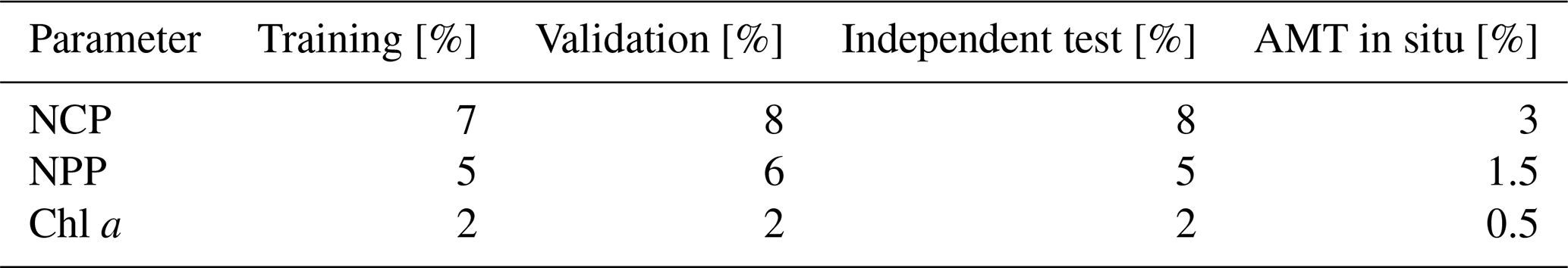
The reduction in pCO_2 (sw) RMSD from reducing input parameter uncertainties by 10 % was also assessed through the perturbation analysis (Table 4). This indicated a decrease in pCO_2 (sw) RMSD of 8 % for NCP, 5 % for NPP and 2 % for Chl a, again indicating that improving NCP uncertainties has the largest impact on improving the estimated pCO_2 (sw) fields.

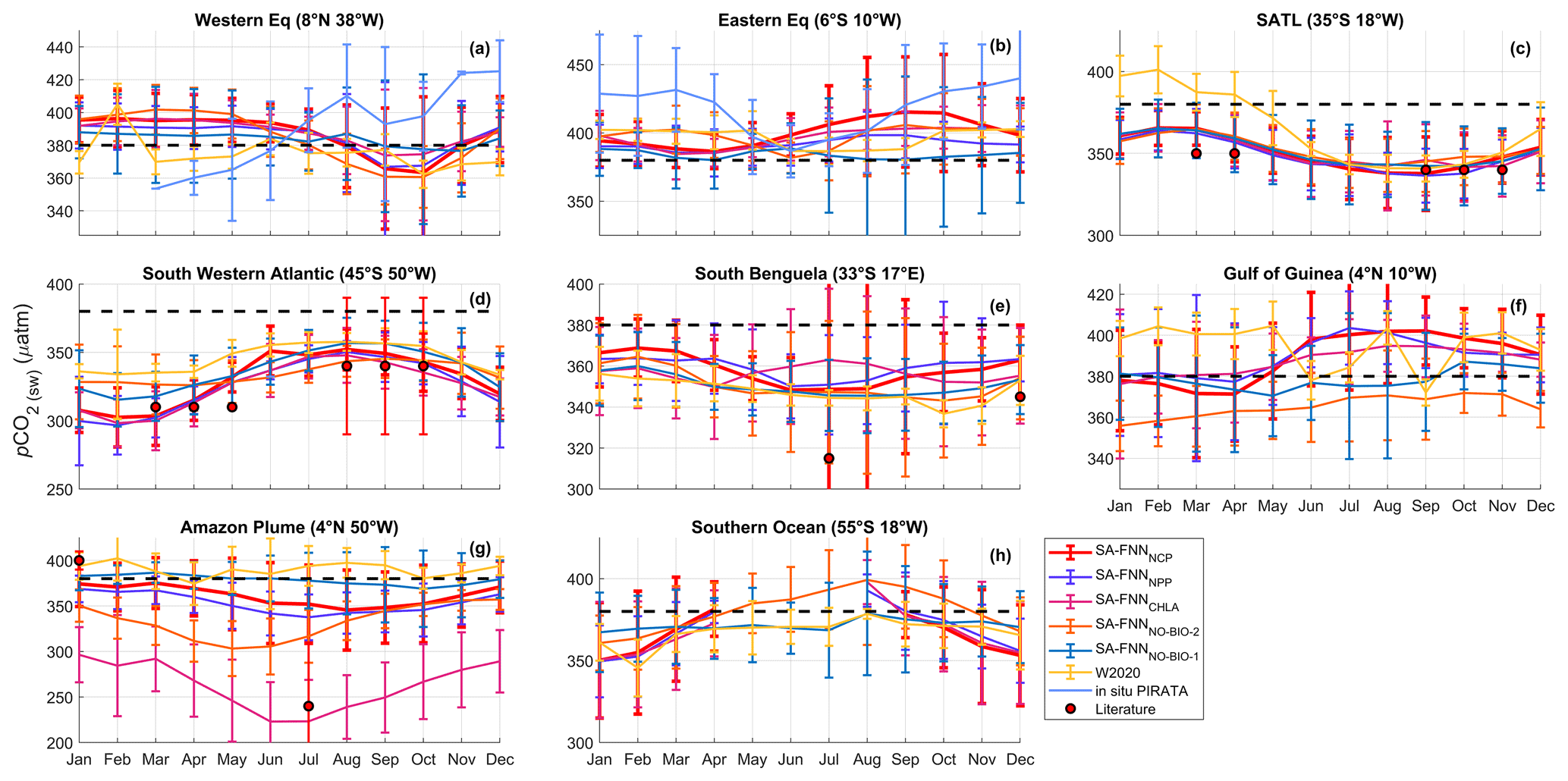
Figure 3 Monthly climatologies of pCO_2 (sw) referenced to the year 2010 for the eight stations marked in Fig. 1 from the SA-FNN_NCP, SA-FNN_NPP, SA-FNN_CHLA, SA-FNN_NO-BIO-1, SA-FNN_NO-BIO-2 and W2020 (Watson et al., 2020b). Light blue lines in Fig. 3a and b indicate the in situ pCO_2 (sw) observations from PIRATA buoys. The atmospheric CO₂ increase was set as 1.5 µatm yr⁻¹. Black dashed line indicates the atmospheric pCO₂ (∼ 380 µatm). Error bars indicate the 2 standard deviations of the climatology (∼ 95 % interval), where larger error bars indicate a larger interannual variability. Red circles indicate the literature values of pCO_2 (sw) described in Sect. 4.2. Note the different y-axis limits in each plot.

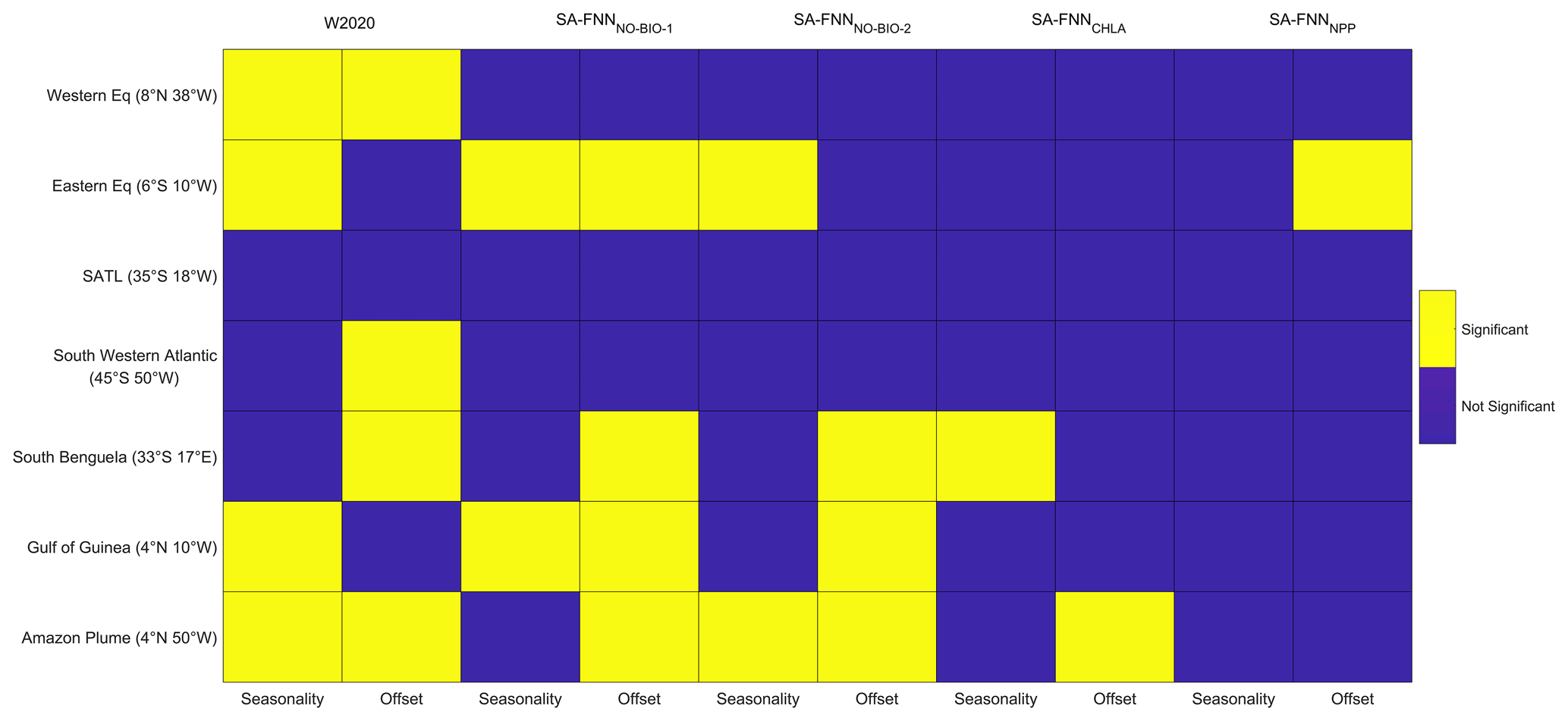
Figure 4 Statistical comparison of the SA-FNN_NCP with the W2020, SA-FNN_NO-BIO-1, SA-FNN_NO-BIO-2, SA-FNN_CHLA and SA-FNN_NPP climatologies, where yellow blocks indicate a significant difference (α=0.05). Seasonality indicates a difference in the seasonal cycle, and offset indicates a difference between the mean pCO_2 (sw) of the climatologies.

3.2 Comparison between SA-FNN_NCP and other methods

The monthly climatologies of pCO_2 (sw) generated using the SA-FNN_NCP and referenced to the year 2010 showed differences with two published climatologies, especially in the equatorial region (Appendix B). The monthly climatology for eight stations (Fig. 1) was extracted from the SA-FNN_NCP, SA-FNN_NPP, SA-FNN_CHLA, SA-FNN_NO-BIO-1, SA-FNN_NO-BIO-2 and the W2020 to assess differences between the pCO_2 (sw) estimates (Fig. 3). The SA-FNN_NCP and SA-FNN_NO-BIO-1 showed significant divergence in the equatorial Atlantic (Figs. 3b, f, g and 4). At the eastern equatorial station, the interannual variability in pCO_2 (sw) from the SA-FNN_NCP was high, and a minimum occurred between January and April, which gradually increased to a maximum in September and October (Fig. 3b). The SA-FNN_NO-BIO-1 showed no seasonality in the pCO_2 (sw) and was consistently below the SA-FNN_NCP pCO_2 (sw). The Gulf of Guinea station showed a similar variability in the SA-FNN_NCP pCO_2 (sw) except that the maxima was lower at this station (Fig. 3f). The SA-FNN_NO-BIO-1 indicated pCO_2 (sw) below the SA-FNN_NCP throughout the year. The greatest divergence occurred near the Amazon Plume (Fig. 3g) where SA-FNN_NCP pCO_2 (sw) was below or at pCO_2 (atm) for all months and there was a large interannual variability in pCO_2 (sw). The SA-FNN_NO-BIO-1 displayed higher pCO_2 (sw) and a lower interannual variability (Fig. 3g).

The SA-FNN_NCP and SA-FNN_NO-BIO-1 showed no significant difference in the seasonal patterns of pCO_2 (sw) at stations south of 20^∘ S (Figs. 3c–e and 4). There was, however, a significant offset at some stations where the SA-FNN_NCP generally exhibited lower pCO_2 (sw) in austral summer and a higher interannual variation. The SA-FNN_NCP was significantly different to W2020 and SA-FNN_NO-BIO-2 at similar stations to those at which SA-FNN_NO-BIO-1 was different (Figs. 3 and 4).

The SA-FNN_NCP and SA-FNN_CHLA showed significant differences in pCO_2 (sw) values in the south Benguela and Amazon Plume. In south Benguela (Figs. 3e and 4), SA-FNN_NCP had pCO_2 (sw) maxima in austral summer, whereas the SA-FNN_CHL maximum occurs in austral winter. In the Amazon Plume there was significant offset between the two methods, and the SA-FNN_CHL resulted in lower pCO_2 (sw) compared to the SA-FNN_NCP (Figs. 3g and 4). The SA-FNN_NCP and SA-FNN_NPP had a significant offset at the eastern equatorial station (Figs. 3c and 4), where the SA-FNN_NPP indicated lower pCO_2 (sw). For the other stations, no significant differences were observed.

4 Discussion

4.1 Assessment of biological parameters to estimate pCO_2 (sw)

In this paper, the differences in estimating pCO_2 (sw) using FNNs with satellite-derived NCP, NPP or Chl a were assessed. The SA-FNN_NCP had an overall accuracy (21.68 µatm; Fig. 2) that is consistent with other approaches that have been developed for the Atlantic (22.83 µatm; Landschützer et al., 2013) and slightly lower than the published global result of 25.95 µatm (Landschützer et al., 2014). Training the SA-FNN using Chl a or NPP showed comparable broadscale accuracy to NCP. When the uncertainties in the input parameters were investigated, however, differences in the estimates of pCO_2 (sw) were apparent. The perturbation analysis indicated that up to a 36 % improvement in estimating pCO_2 (sw) could be achieved if NCP data uncertainties were reduced (Table 3). A similar improvement could be obtained if the NPP uncertainties were reduced (Table 3). Ford et al. (2021b) showed that up to 40 % of the uncertainty in satellite NCP is attributed to the uncertainty in satellite NPP, which is an input to the NCP approach. This suggests that improvements in estimating NPP from satellite data will lead to a further improvement in estimating pCO_2 (sw) from NCP. These improvements could be achieved through better estimates of the water column light field (e.g. Sathyendranath et al., 2020) and the vertical variability of input parameters or assignment of photosynthetic parameters (e.g. Kulk et al., 2020), for example. For a discussion on improving satellite NPP estimates we refer the reader to Lee et al. (2015).

To uncouple the Chl a, NPP, and NCP estimates and their uncertainties, the perturbation analysis was also conducted on Atlantic Meridional Transect in situ observations. This showed that reducing in situ NCP uncertainties provided the greatest reduction in pCO_2 (sw) RMSD, which was 3 times the reduction achievable using Chl a (Tables 3 and 4). This indicates that the optimal predictive power of Chl a to estimate pCO_2 (sw) has been reached and that to achieve further improvements in estimates of pCO_2 (sw) and reduction in its associated uncertainty requires the use of NCP.

A reduction of input uncertainties to ∼ 0 is near impossible, but a reduction by 10 % could be feasible (e.g. NCP uncertainty reduced from 45 to 40.5 $\mathrm{mmol}{\mathrm{O}}_{\mathrm{2}}{\mathrm{m}}^{-\mathrm{2}}{\mathrm{d}}^{-\mathrm{1}}$; Table 1). A perturbation analysis conducted for this showed similar results, with NCP producing the greatest reduction in pCO_2 (sw) RMSD of 8 % compared to 2 % for Chl a (Table 4). Thus, reducing NCP uncertainties will provide a greater improvement in pCO_2 (sw) compared to reducing the uncertainties in Chl a.

These improvements in estimating NCP could be achieved through many components. Ford et al. (2021b) showed that 40 % of satellite NCP uncertainties were attributed to in situ NCP uncertainties. The in situ bottle incubation measurements could be improved using the principles of Fiducial Reference Measurements (FRM; Banks et al., 2020), which are traceable to metrology standards, referenced to inter-comparison exercises, with a full uncertainty budget. This becomes complicated, however, when considering the number of different methods to measure NCP and the large divergence between them (Robinson et al., 2009). A review of these methods has already been conducted (Duarte et al., 2013; Ducklow and Doney, 2013; Williams et al., 2013). The methods broadly fall into the following categories: (a) in vitro incubations of samples under light/dark treatments (Gist et al., 2009) and (b) in situ observations of oxygen-to-argon (${\mathrm{O}}_{\mathrm{2}}/\mathrm{Ar}$) ratios (Kaiser et al., 2005) or the observed isotopic signature of oxygen (Kroopnick, 1980; Luz and Barkan, 2000). All of these methods are subject to, but do not account for, the photochemical sink, which may lead to underestimation of in vitro NCP by up to 22 % (Kitidis et al., 2014). Independent ground measurements that use accepted protocols for the in vitro method are currently made on the Atlantic Meridional Transect; however, a community consensus should consider a consistent methodology for NCP. Increasing the number of such observations for the purpose of algorithm development would further constrain the NCP but also provide observations across the lifetime of newly launched satellites. The uncertainties on each in vitro measurement are assessed through replicate bottles which could be used to calculate a full uncertainty budget for each NCP measurement when combined with analytical uncertainties.

Serret et al. (2015) indicated that NCP is controlled by both the heterogeneity in NPP and respiration. The satellite NCP algorithm applied in this study accounts for some of the heterogeneity in respiration, through an empirical SST-to-NCP relationship (Tilstone et al., 2015). Quantifying the variability in respiration could further improve NCP estimates when coupled with NPP rates from satellite observations.

4.2 Accuracy of SA-FNN_NCP pCO_2 (sw) at seasonal and interannual scales

The seasonal and interannual variability of pCO_2 (sw) estimated using the SA-FNN_NCP was compared with the SA-FNN_NO-BIO, W2020 (Watson et al., 2020b), SA-FNN_CHL and SA-FNN_NPP at eight stations. The stations (Fig. 1) represent locations of previous studies into in situ pCO_2 (sw) variability, allowing comparisons with literature values. Significant differences between the SA-FNN_NCP and SA-FNN_NO-BIO were observed at four stations (Fig. 4), especially in the equatorial Atlantic.

At 8^∘ N, 38^∘ W (Fig. 3a), Lefèvre et al. (2020) reported pCO_2 (sw) to be stable at ∼ 400 µatm, between June and August 2013, and to decrease in September to ∼ 360 µatm, which is attributed to the Amazon Plume propagating into the western equatorial Atlantic (Coles et al., 2013). Bruto et al. (2017) indicated, however, that elevated pCO_2 (sw) at ∼ 430 µatm was observed in September for 2008 to 2011. The error bars on the PIRATA buoy pCO_2 (sw) observations (Fig. 3a) clearly highlight the differences between Lefèvre et al. (2020) and Bruto et al. (2017), but there are less than 4 years of monthly observations available, which do not resolve the full seasonal cycle. For the station in the Amazon Plume at 4^∘ N, 50^∘ W (Fig. 3g), where the effects of the plume extend northwest towards the Caribbean (Coles et al., 2013; Varona et al., 2019), Lefèvre et al. (2017) indicated that this region acts as a sink for CO₂ (pCO_2 (sw) < pCO_2 (atm)), especially between May and July, coincident with maximum discharge from the Amazon River (Dai and Trenberth, 2002). Valerio et al. (2021) indicated pCO_2 (sw) varied at and below pCO_2 (atm) at 4^∘ N, 50^∘ W, consistent with the SA-FNN_NCP. The interannual variability of pCO_2 (sw) has been shown to be high in this region in all months (Lefèvre et al., 2017). The SA-FNN_NCP provided a better representation of the seasonal and interannual variability induced by the Amazon River discharge and associated plume at these two stations compared to the SA-FNN_NO-BIO, although differences were small at 8^∘ N, 38^∘ W.

The station in the eastern tropical Atlantic at 6^∘ S, 10^∘ W (Fig. 3b) is under the influence of the equatorial upwelling (Lefèvre et al., 2008), which is associated with the upwelling of CO₂-rich waters between June and September. Lefèvre et al. (2008) indicated that peak pCO_2 (sw) of ∼ 440 µatm was observed in September and remained stable until December, before decreasing to a minima of ∼ 360 µatm in May (Parard et al., 2010). Lefèvre et al. (2016) showed, however, that the influence of the equatorial upwelling does not reach the buoy in all years, and in some years lower pCO_2 (sw) is observed. The PIRATA buoy observations (Fig. 3b) clearly show this seasonality but also highlight the interannual variability in in situ pCO_2 (sw). Further north at 4^∘ N, 10^∘ W (Fig. 3f), Koffi et al. (2010) suggested that this region follows a similar seasonal cycle as the station at 6^∘ S, 10^∘ W but that pCO_2 (sw) is ∼ 30 µatm lower (Koffi et al., 2016). The interannual variability in SA-FNN_NCP pCO_2 (sw) clearly shows the influence of the equatorial upwelling at these stations, with latitudinal gradients in pCO_2 (sw) during the upwelling period (Lefèvre et al., 2016), but struggles to identify elevated pCO_2 (sw) between December and April shown by the PIRATA buoy observations (Fig. 3b). By contrast, the SA-FNN_NO-BIO-1 indicated little influence from the equatorial upwelling and a depressed pCO_2 (sw) during the upwelling season.

The two methods converge on the seasonal cycle at the remaining stations, although significant offsets in the mean annual pCO_2 (sw) remain. The station at 35^∘ S, 18^∘ W (Fig. 3c) has consistently been implied as a sink for CO₂. Lencina-Avila et al. (2016) showed the region to have 340 µatm pCO_2 (sw) and to be a sink for CO₂ between October and December. Similarly, Kitidis et al. (2017) implied that the region is a sink for CO₂ during March to April. The region has depressed pCO_2 (sw) due to high biological activity that originates from the Patagonian Shelf and the South Subtropical Convergence Zone. The station at 45^∘ S, 50^∘ W (Fig. 3d) has also been implied as a strong but highly variable sink, where pCO_2 (sw) can be between ∼ 280 and ∼ 380 µatm during austral spring and is constant at ∼ 310 µatm during austral autumn (Kitidis et al., 2017). The SA-FNN_NCP and SA-FNN_NO-BIO-1 methods reproduced the seasonal variability in the pCO_2 (sw) at these two stations accurately, but only the SA-FNN_NCP captures the magnitude of the depressed pCO_2 (sw) at 45^∘ S.

Within the southern Benguela upwelling system, pCO_2 (sw) at station 33^∘ S, 17^∘ E (Fig. 3e) is influenced by gradients in the seasonal upwelling (Hutchings et al., 2009). Santana-Casiano et al. (2009) showed that pCO_2 (sw) varies from ∼ 310 µatm in July to ∼ 340 µatm in December and that the region is a CO₂ sink through the year. González-Dávila et al. (2009) suggested, however, that this CO₂ sink is highly variable during upwelling events and that recently upwelled waters act as a source (pCO_2 (sw) > pCO_2 (atm)) of CO₂ to the atmosphere (Gregor and Monteiro, 2013). Arnone et al. (2017) indicated elevated pCO_2 (sw) during austral spring and autumn at the station, with a ∼ 40 µatm seasonal cycle amplitude. The SA-FNN_NCP and SA-FNN_NO-BIO-1 were able to reproduce the seasonal cycle, although the SA-FNN_NCP correctly represented the seasonal magnitude in pCO_2 (sw) as reported by Santana-Casiano et al. (2009) and Arnone et al. (2017).

In summary, for these stations, the SA-FNN_NCP better represents the seasonality and the interannual variability of pCO_2 (sw) in the South Atlantic Ocean compared to the SA-FNN_NO-BIO-1, especially in the equatorial Atlantic. The SA-FNN_NO-BIO-2 also displayed significant differences compared to SA-FNN_NCP, indicating that the variability in pCO_2 (sw) has a strong biological contribution which is not fully represented and explained by the additional physical parameters included in the FNN. The SA-FNN_NO-BIO-2 and W2020 both displayed significant differences compared to the SA-FNN_NCP at specific stations (Fig. 4). There are methodological differences between these approaches, however. The SA-FNN method uses only in situ pCO_2 (sw) observations from the South Atlantic Ocean to train the FNNs. The W2020 uses global in situ pCO_2 (sw) observations to train FNNs for 16 provinces with similar seasonal cycles (Landschützer et al., 2014; Watson et al., 2020b). The W2020 will therefore be weighted to pCO_2 (sw) variability in regions of relatively abundant in situ observations (i.e. Northern Hemisphere) and may not be fully representative of the South Atlantic Ocean. This would explain the SA-FNN_NO-BIO-2 and W2020 differences, when driven using the same input variables.

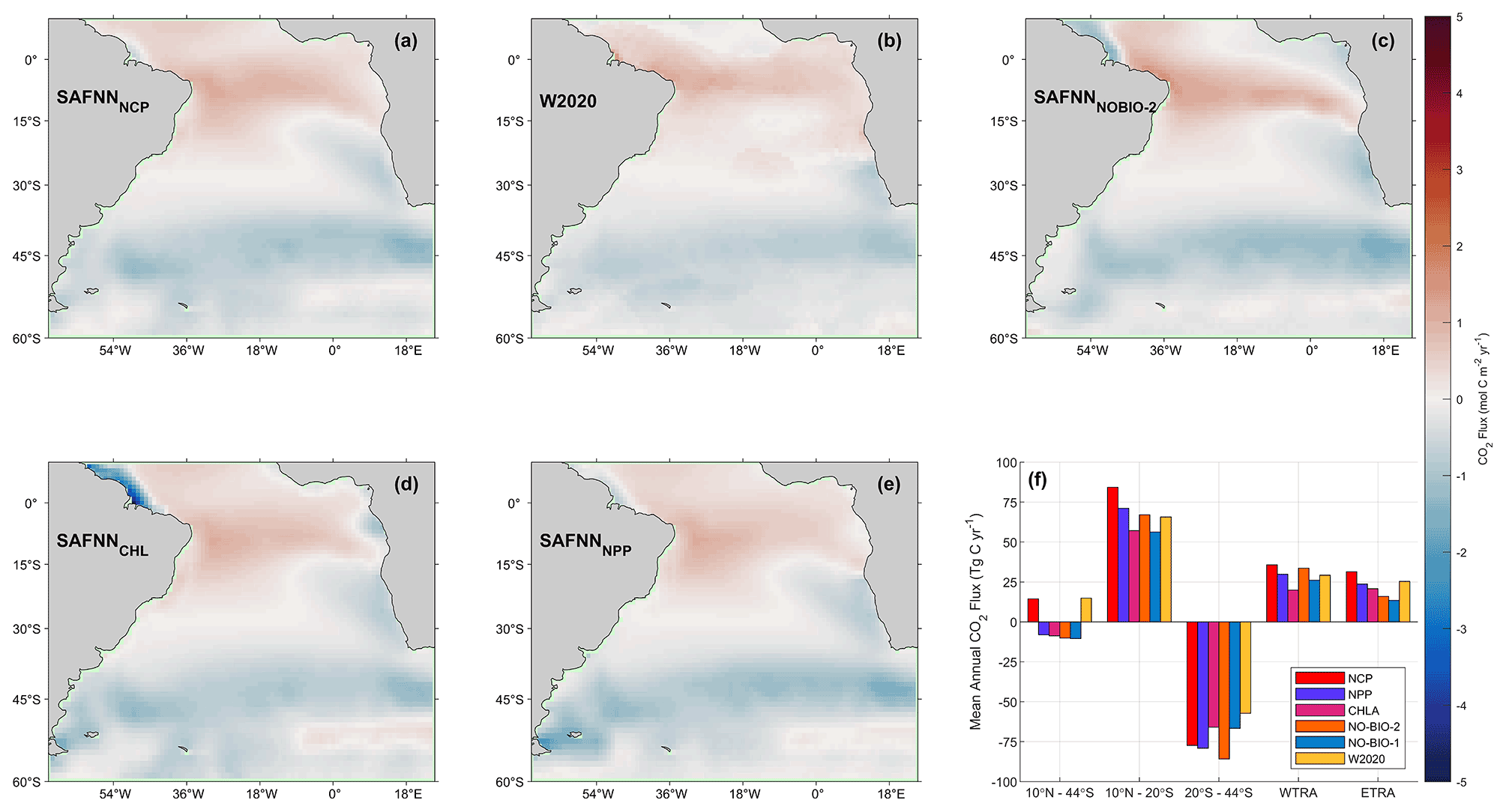
Figure 5 Long-term average annual mean CO₂ flux for the South Atlantic Ocean, using pCO_2 (sw) estimates from (a) SA-FNN_NCP, (b) W2020 (Watson, et al., 2020a), (c) SA-FNN_NO-BIO-2, (d) SA-FNN_CHLA and (e) SA-FNN_NPP. (f) Bar chart displaying the mean annual CO₂ flux for different regions of the South Atlantic Ocean including 10^∘ N to 44^∘ S (whole South Atlantic Ocean), 10^∘ N to 20^∘ S, and 20 to 44^∘ S, alongside the WTRA and ETRA biogeochemical provinces (Fig. 1a).

Comparing the SA-FNN_NCP and SA-FNN_CHLA there were two significant differences (Fig. 4). A difference in the seasonal cycle in the southern Benguela (Fig. 3e) was observed. Santana-Casiano et al. (2009) showed that the minima pCO_2 (sw) in July and maxima in December, consistent with the SA-FNN_NCP and SA-FNN_NPP, whereas the SA-FNN_CHL estimated the opposite scenario. Lamont et al. (2014) reported Chl a concentrations to remain consistent in May and October, but NPP rates were significantly higher in October, associated with increased surface PAR and enhanced upwelling. The disconnect between Chl a and NPP can also be observed in the satellite observations (Appendix C Fig. C1), limiting the ability of Chl a to estimate pCO_2 (sw), which is highlighted by the failure of the SA-FNN_CHLA to identify the seasonal pCO_2 (sw) cycle.

A Chl a-to-NPP disconnect has also been reported in the Amazon Plume (Smith and Demaster, 1996), where Chl a concentrations can be similar but NPP rates significantly different due to light limitation caused by suspended sediments. A significant offset between the SA-FNN_NCP and SA-FNN_CHLA was observed in this region (Figs. 3g and 4). Lefèvre et al. (2017) reported pCO_2 (sw) values ranging from 400 ± ∼ 10 µatm in January to ∼ 240 ± ∼ 70 µatm in May. Although, the SA-FNN_NCP January estimates are consistent, the May estimates are higher than these in situ measurements. These observations were made further north (6^∘ N) where the turbidity within the plume has decreased sufficiently for irradiance to elevate NPP rates (Smith and Demaster, 1996), which decrease pCO_2 (sw). Chl a remains relatively consistent across the plume (not shown), suggesting a disconnect between Chl a and NPP at 4^∘ N, 50^∘ W, which would lead to lower pCO_2 (sw) estimates by the SA-FNN_CHLA, where NPP rates are low due to light limitation (Chen et al., 2012; Smith and Demaster, 1996). Respiration would be elevated from the decomposition of riverine organic material reducing NCP further (Cooley et al., 2007; Jiang et al., 2019; Lefèvre et al., 2017). It is noted that the Amazon Plume is a dynamic region with transient, localised biological and pCO_2 (sw) features (Cooley et al., 2007; Ibánhez et al., 2015; Lefèvre et al., 2017; Valerio et al., 2021) that may be masked by the coarse resolution of estimates available using satellite data. The SA-FNN_NCP, however, agreed with in situ pCO_2 (sw) observations at 4^∘ N, 50^∘ W, where pCO_2 (sw) varied at or below pCO_2 (atm) (Valerio et al., 2021).

Though the differences between the SA-FNN_NCP and SA-FNN_CHLA may appear small, the Amazon Plume and Benguela Upwelling have a higher intensity in the CO₂ flux per unit area compared to the open ocean, illustrating a disproportionate contribution to the overall global CO₂ sink than their small areal coverage implies (Laruelle et al., 2014). The differences in the pCO_2 (sw) estimates result in a 22 Tg C yr⁻¹ alteration in the annual CO₂ flux for the South Atlantic Ocean (SA-FNN_NCP = +14 Tg C yr⁻¹; SA-FNN_CHLA = −9 Tg C yr⁻¹; Fig. 5f). This unequivocally reinforces the use of NCP to improve basin-scale estimates of pCO_2 (sw), especially in regions where Chl a, NPP and NCP become disconnected.

Recent assessments of the strength of the global oceanic CO₂ sink have been made using pCO_2 (sw) fields estimated using no biological parameters as input (Watson et al., 2020b). Our results indicate that the SA-FNN_NCP more accurately represented the pCO_2 (sw) variability in the South Atlantic Ocean compared to the SA-FNN_NO-BIO-2, which included additional physical parameters. Estimating the South Atlantic Ocean net CO₂ flux with the SA-FNN_NCP pCO_2 (sw) produced a 14 Tg C yr⁻¹ source compared to a 10 Tg C yr⁻¹ sink indicated by the SA-FNN_NO-BIO-2 (Fig. 5f). The incremental inclusion of parameters to account for the biological signal starting with Chl a (−9 Tg C yr⁻¹), then NPP (−7 Tg C yr⁻¹) and then NCP (+14 Tg C yr⁻¹) switched the South Atlantic Ocean from a CO₂ sink to a source, which is driven by differences in the pCO_2 (sw) estimates in regions that are biologically controlled. This 21 Tg C yr⁻¹ difference between the SA-FNN_NCP and SA-FNN_NPP is due to additional outgassing in the equatorial Atlantic provinces of the WTRA and ETRA (Figs. 1a and 5f). Compared to the in situ pCO_2 (sw) observations at the equatorial stations (Fig. 3a and b), it is likely that the outgassing is still underestimated by the SA-FNN_NCP but does improve these estimates within the upwelling season (June–September).

The W2020 identified the South Atlantic Ocean as a source for CO₂ of 15 Tg C yr⁻¹, which is consistent with the SA-FNN_NCP (Fig. 5f). The SA-FNN_NCP, however, indicated the equatorial Atlantic (10^∘ N to 20^∘ S) as a 20 Tg C yr⁻¹ stronger source and south of 20^∘ S (20^∘ S to 44^∘ S) as a 20 Tg C yr⁻¹ stronger sink. These differences indicate that biologically induced variability in pCO_2 (sw) would not be captured by the W2020 and could reduce the variability in the global ocean CO₂ sink. A further SA-FNN trained with pCO_2 (atm), SST, salinity, mixed layer depth and NCP indicated a similar CO₂ source of 12 Tg C yr⁻¹ (data not shown) as the SA-FNN_NCP for the South Atlantic Ocean, highlighting that additional physical parameters cannot fully account for the biological contribution to the variability in pCO_2 (sw). This further confirms the importance of using NCP within estimates of the global ocean CO₂ sink.

5 Conclusions

In this paper, we compare neural network models of pCO_2 (sw) parameterised separately using either satellite Chl a, NPP or NCP as biological proxies to estimate complete fields of pCO_2 (sw). The results suggest that using NCP improved the estimation of pCO_2 (sw). The differences between satellite Chl a, NPP or NCP were initially small, but the use of a perturbation analysis to assess the uncertainties in these parameters showed that NCP has a greater potential uncertainty reduction of up to ∼ 36 % of the RMSD, compared to a ∼ 19 % for Chl a. These results were verified using in situ observations from the Atlantic Meridional Transect, which resulted in a 25 % improvement in pCO_2 (sw) RMSD when the in situ NCP uncertainties were reduced to ∼ 0, compared to 7 % for Chl a and 13 % for NPP.

Monthly climatological estimates of pCO_2 (sw) at eight stations in the South Atlantic Ocean, calculated using satellite NCP, were compared with the NPP and the Chl a approaches and two neural networks that do not use biological parameters. The NCP approach significantly improved on both approaches with no biological parameters at four stations in reconstructing the seasonal and interannual variability, compared to in situ pCO_2 (sw) observations. At the remaining four stations, differences were also observed, although these were not statistically significant. In the eastern equatorial Atlantic, in the upwelling region, a significant difference between the NCP and NPP approaches occurred. Significant differences between the NCP and Chl a approaches were also observed in the Benguela upwelling and Amazon Plume, where pCO_2 (sw) from Chl a suggested that photosynthetic rates were not solely controlled by Chl a. Using NCP to estimate pCO_2 (sw) the South Atlantic Ocean was characterised as a net source of CO₂, whereas methods that only include physical controls have indicated the region to be a small sink for CO₂. Sequentially using Chl a to estimate pCO_2 (sw) and then NPP incrementally reduced the South Atlantic CO₂ sink, and finally using NCP the area switched to being a source of CO₂. These results indicate that in regions where biological activity is important in controlling the variability in pCO_2 (sw), the use of NCP, which is available from satellite data, is important for quantifying the ocean carbon pump and for providing data in areas that are sparsely covered by observations such as the Southern Ocean.

Appendix A: Feed forward neural network training and perturbation analysis

Table A1 The percentage reduction in root mean square difference (RMSD) attributable to the uncertainties in the input parameter for each training and validation data set determined from a perturbation analysis as described in Sect. 2.5.

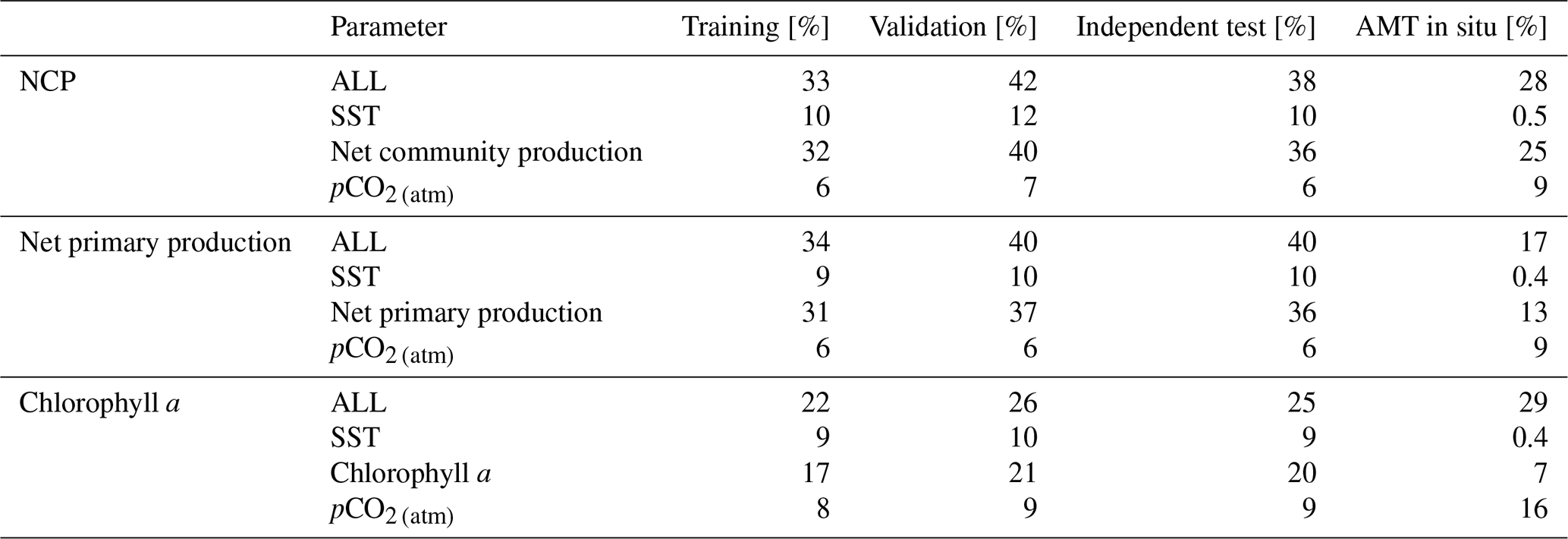
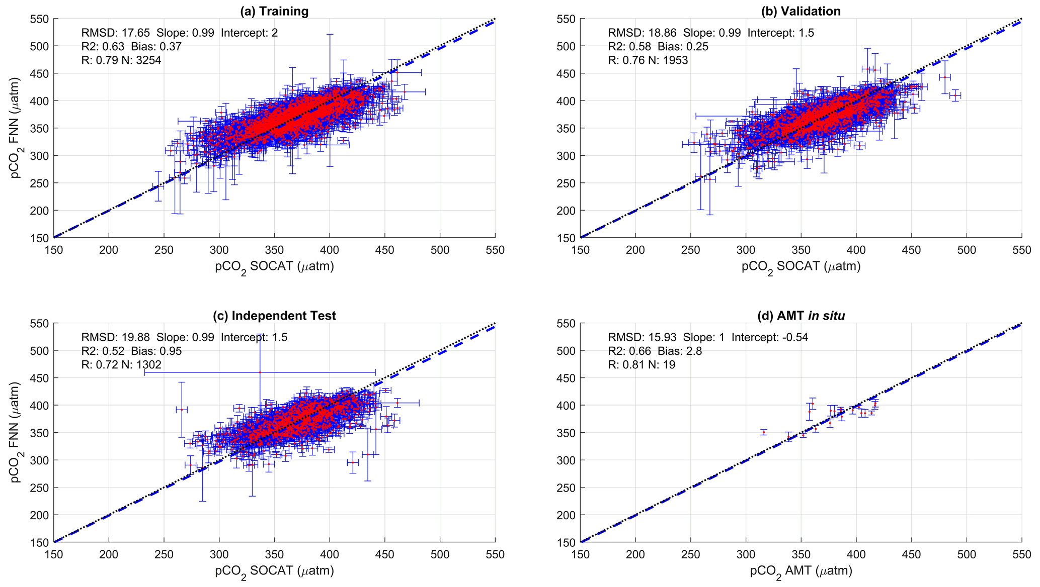
Figure A1 Scatter plots showing the combined performance of the eight feed forward neural networks trained using chlorophyll a for four separate training and validation datasets: (a) training, (b) validation, (c) independent test and (d) Atlantic Meridional Transect (AMT) in situ. The blue dashed line is the type II regression, and the black dashed line is the 1:1 line. Horizontal error bars indicate the uncertainty of the SOCATv2020 pCO_2 (sw). Vertical error bars indicate the uncertainty attributed to the input parameter uncertainty propagated through the feed forward neural networks. The statistics within each plot are the root mean square difference (RMSD), slope and intercept of the type II regression, coefficient of determination (R²), Pearson correlation coefficient (R), bias and number of samples (N).

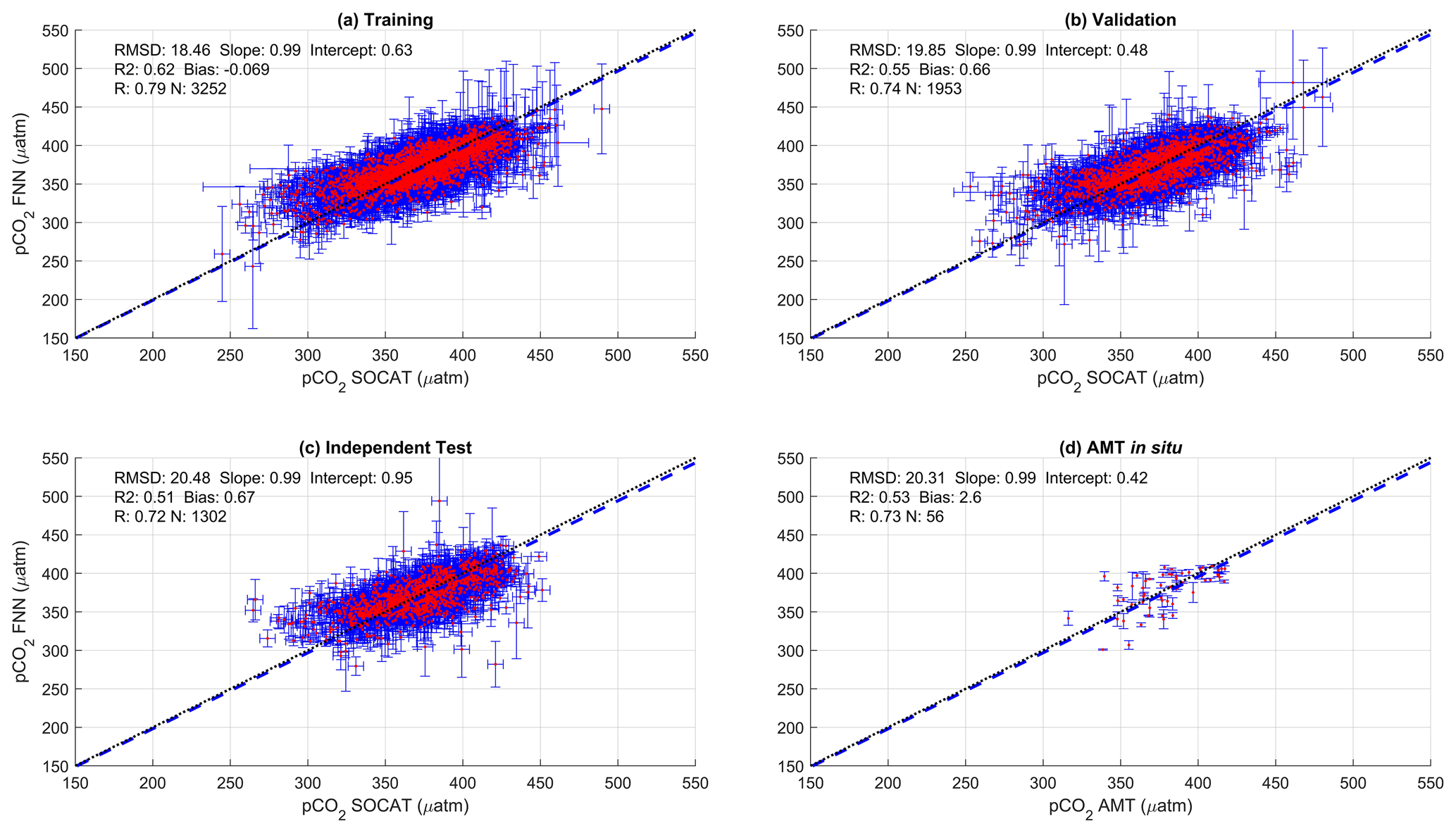
Figure A2 Scatter plots showing the combined performance of the eight feed forward neural networks trained using net primary production for four separate training and validation datasets: (a) training, (b) validation, (c) independent test and (d) Atlantic Meridional Transect (AMT) in situ. The blue dashed line is the type II regression, and the black dashed line is the 1:1 line. Horizontal error bars indicate the uncertainty of the SOCATv2020 pCO_2 (sw). Vertical error bars indicate the resulting uncertainty attributed to the input parameter uncertainty propagated through the feed forward neural networks. The statistics within each plot are the root mean square difference (RMSD), slope and intercept of the type II regression, coefficient of determination (R²), Pearson correlation coefficient (R), bias and number of samples (N).

Figure A3 Scatter plots showing the combined performance of the eight feed forward neural networks trained using no biological parameters (SA-FNN_NO-BIO-1) for three separate training and validation datasets: (a) training, (b) validation and (c) independent test. The blue dashed line is the type II regression, and the black dashed line is the 1:1 line. Horizontal error bars indicate the uncertainty of the SOCATv2020 pCO_2 (sw). Vertical error bars indicate the resulting uncertainty attributed to the input parameter uncertainty propagated through the feed forward neural networks. The statistics within each plot are the root mean square difference (RMSD), slope and intercept of the type II regression, coefficient of determination (R²), Pearson correlation coefficient (R), bias and number of samples (N).

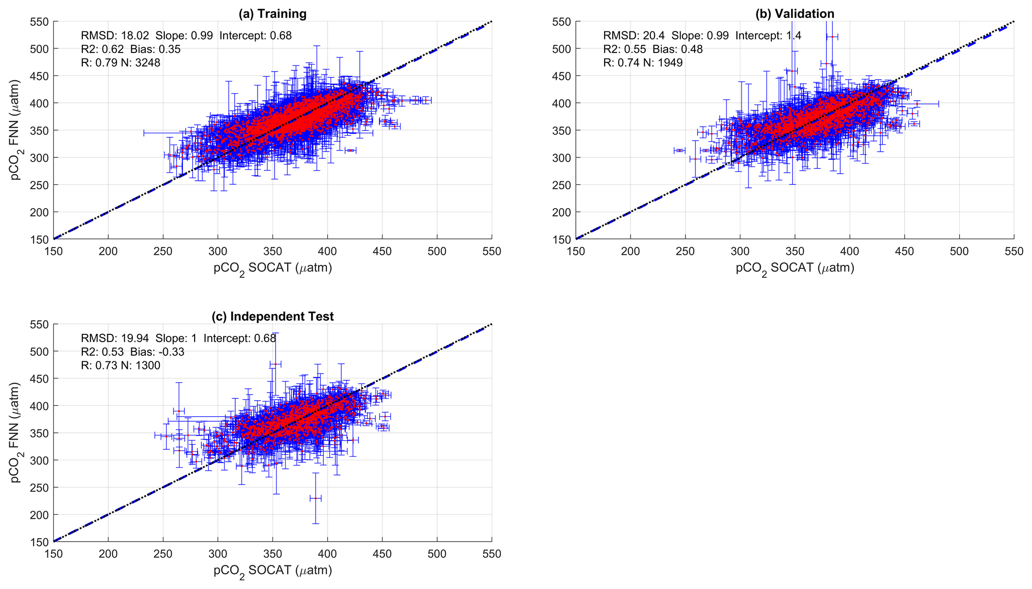
Figure A4 Scatter plots showing the combined performance of the eight feed forward neural networks trained using no biological parameters (SA-FNN_NO-BIO-2) for three separate training and validation datasets: (a) training, (b) validation and (c) independent test. The blue dashed line is the type II regression, and the black dashed line is the 1:1 line. Horizontal error bars indicate the uncertainty of the SOCATv2020 pCO_2 (sw). Vertical error bars indicate the resulting uncertainty attributed to the input parameter uncertainty propagated through the feed forward neural networks. The statistics within each plot are the root mean square difference (RMSD), slope and intercept of the type II regression, coefficient of determination (R²), Pearson correlation coefficient (R), bias and number of samples (N).

Appendix B: Climatology comparison

A monthly climatology was generated from the SA-FNN_NCP monthly time series (Fig. B1), referenced to the year 2010, assuming an atmospheric CO₂ increase of 1.5 µatm yr⁻¹ (Takahashi et al., 2009; Zeng et al., 2014). The standard deviation of the monthly climatology was computed, as an indication of the interannual variations in the climatology. The ability of the SA-FNN_NCP to estimate the spatial distribution of pCO_2 (sw) was compared to two methods.

Firstly, the SA-FNN_NCP climatology was compared to the climatology from Woolf et al. (2019), produced following the statistical “ordinary block kriging” approach described in Goddijn-Murphy et al. (2015), using the SOCATv4 reanalysed data. The method provides an interpolation uncertainty where in regions of sparse data this becomes larger. Figure B2 shows the methods produce similar climatological pCO_2 (sw) values for the South Atlantic Ocean, with some clear differences along the African coastline, and equatorial region.

Secondly, the SA-FNN_NCP was compared to a climatology calculated from the standard method, a self-organising-map feed forward neural network presented in Watson et al. (2020b; W2020). Figure B3 shows the methods produce similar climatological pCO_2 (sw) values for the South Atlantic Ocean; however, clear differences in the equatorial region occur across all months. In the central South Atlantic Ocean, artefacts form the self-organising map can be seen during January and February.

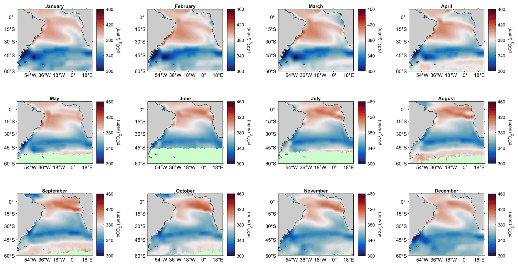
Figure B1 Monthly climatologies of pCO_2 (sw) between July 2002 and December 2018 estimated by the SA-FNN_NCP approach referenced to 2010. The atmospheric CO₂ increase was set as 1.5 µatm yr⁻¹. The colour scale is centred on the atmospheric concentration for 2010 (∼ 380 µatm). Red shaded areas indicate oversaturated regions, and blue shaded areas indicate undersaturated regions. Light green areas indicate where no input data to compute pCO_2 (sw) are available.

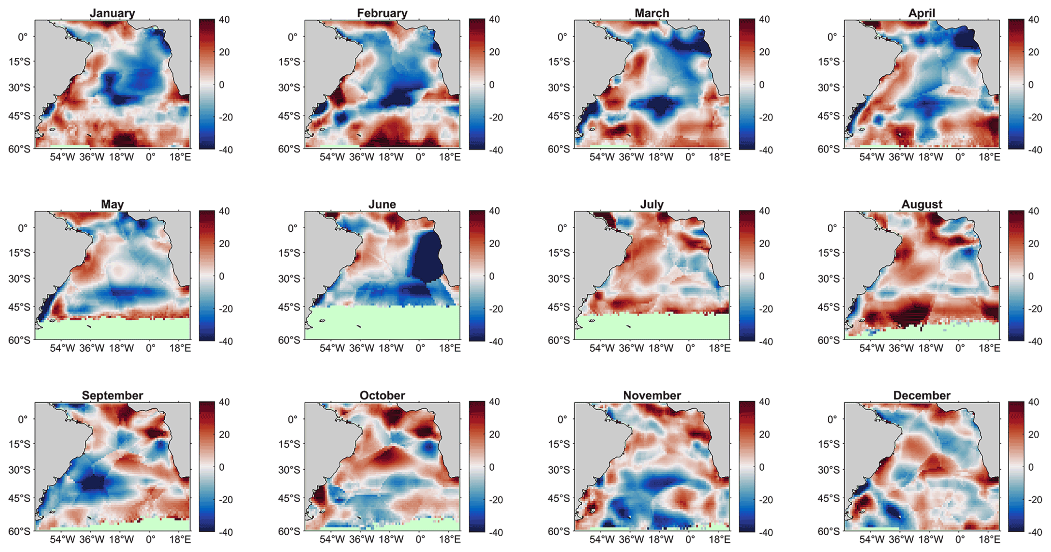
Figure B2 Monthly comparison between pCO_2 (sw) climatology estimated by the SA-FNN_NCP and Woolf et al. (2019) climatology referenced to 2010 (SA-FNN_NCP pCO₂ – Woolf pCO₂). Red (Blue) shades indicate regions where SA-FNN is greater (less) than the Woolf climatology.

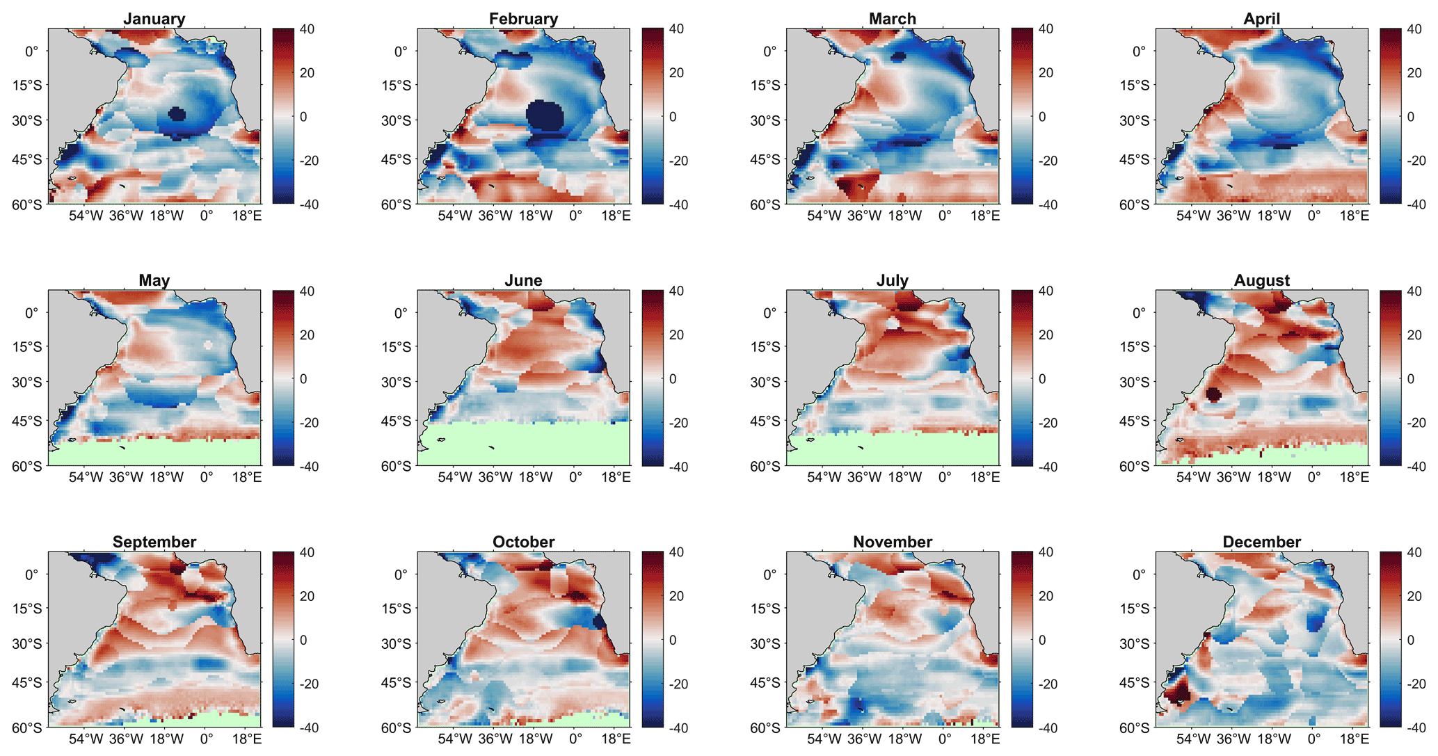
Figure B3 Monthly comparison between pCO_2 (sw) climatologies estimated by the SA-FNN_NCP and W2020 (Watson et al., 2020a) climatology referenced to 2010 (SA-FNN_NCP pCO₂ – W2020 pCO₂). Red (Blue) shades indicate regions where SA-FNN_NCP is greater (less) than the W2020 climatology.

Appendix C: Biological parameter climatologies

Figure C1 Monthly climatologies of the biological parameters (Chl a, NPP and NCP) for the eight stations (Fig. 1a). Chl a and NPP scale on the left axis, and NCP on the right. Note the different axis limits on each plot.