Benthic macrofaunal carbon fluxes and environmental drivers of spatial variability in a large coastal-plain estuary

While the importance of carbon cycling in estuaries is increasingly recognized, the role of benthic macrofauna remains poorly quantified due to limited spatial and temporal resolution in biomass measurements. Here, we ask: (1) To what extent do benthic macrofauna contribute to estuarine carbon cycling via respiration and calcification? and (2) How well can routinely collected environmental variables predict their biomass? We analyzed data from 8128 benthic samples collected from the Chesapeake Bay between 1995 and 2022 and estimated associated carbon fluxes using empirical relationships. We then used generalized additive models to relate observed and modeled environmental variables to the biomass. Biomass was highest in the upper mainstem of the Bay (Upper Bay) and upper Potomac River Estuary, the largest tidal tributary of the Bay. In the Upper Bay, benthic macrofauna respired 18 %–45 % of the estimated organic carbon supply. Calcification-driven alkalinity reduction reached 6.31 ± 2.84 mol m⁻² yr⁻¹ in the Potomac River Estuary, aligning with prior estimates of alkalinity sinks in the tributary and highlighting the potential importance of calcifying fauna in alkalinity dynamics. Estimated CO₂ production in the Upper Bay from benthic respiration and calcification (151 g C m⁻² yr⁻¹) also exceeded observed air–sea CO₂ fluxes (74.5 g C m⁻² yr⁻¹). Generalized additive models revealed that low salinity, moderate dissolved oxygen, and elevated nitrate best predicted high-biomass zones, with the three predictors explaining 52 % of biomass deviance. These predictive relationships offer a pathway to estimate macrofaunal biomass and associated carbon fluxes in systems where direct biomass measurements are sparse. Our findings demonstrate that benthic macrofauna play a substantial and spatially structured role in estuarine carbon cycling. Incorporating their contributions into estuarine biogeochemical models will improve predictions of ecosystem responses to environmental and anthropogenic change.

1 Introduction

Benthic macrofauna are vitally important to estuarine ecosystems by improving water quality, producing and consuming organic matter, recycling nutrients, cycling pollutants, stabilizing and transporting sediment, and providing food for both human populations and estuarine organisms (Schratzberger and Ingels, 2018; Snelgrove, 1997; Wilson and Fleeger, 2023). Benthic macrofauna also play a role in estuarine carbon cycling through secondary production, respiration, and calcification. Secondary production refers to the consumption of organic matter by benthos to produce soft tissue biomass (Diaz and Schaffner, 1990; Dolbeth et al., 2012; Sturdivant et al., 2013). This biomass contributes to trophic transfer, as benthic organisms are consumed by predators or decomposers, with much of the associated organic carbon eventually being removed from the estuary through advection to the open ocean or burial in sediment (Diaz and Schaffner, 1990; Wilson and Fleeger, 2023). Respiration and calcification influence carbon cycling through their impact on the carbonate system, the chemical equilibrium governing the partitioning of inorganic carbon among its primary forms.

Impacts of respiration and calcification on the carbonate system are best understood via their impacts on two master variables, dissolved inorganic carbon (DIC) and total alkalinity (TA). DIC is a measure of the total concentration of inorganic carbon species in water, including carbon dioxide, bicarbonate ion, and carbonate ion:

$$\begin{array}{}\text{(1)}& \left[\mathrm{DIC}\right]=\left[{\mathrm{CO}}_{\mathrm{2}}\right]+\left[{\mathrm{HCO}}_{\mathrm{3}}^{-}\right]+\left[{\mathrm{CO}}_{\mathrm{3}}^{\mathrm{2}-}\right].\end{array}$$

TA is the excess of proton acceptors over donors and reflects the capacity of a water body to buffer pH changes. For understanding impacts of biogeochemical processes, the form of TA known as the explicit conservative alkalinity (Glud, 2008; Wolf-Gladrow et al., 2007) is useful:

$$\begin{array}{}\text{(2)}& \begin{array}{rl}\left[\mathrm{TA}\right]& =\left[{\mathrm{Na}}^{+}\right]+\mathrm{2}\left[{\mathrm{Mg}}^{\mathrm{2}+}\right]+\mathrm{2}\left[{\mathrm{Ca}}^{\mathrm{2}+}\right]+\left[{\mathrm{K}}^{+}\right]\\ & +\mathrm{2}\left[{\mathrm{Sr}}^{\mathrm{2}+}\right]+\mathrm{\dots }-\left[{\mathrm{Cl}}^{-}\right]-\left[{\mathrm{Br}}^{-}\right]-\left[{\mathrm{NO}}_{\mathrm{3}}^{-}\right]\\ & -\mathrm{\dots }-{\mathrm{TPO}}_{\mathrm{4}}+{\mathrm{TNH}}_{\mathrm{3}}-\mathrm{2}{\mathrm{TSO}}_{\mathrm{4}}-\mathrm{THF}\\ & -{\mathrm{THNO}}_{\mathrm{2}},\end{array}\end{array}$$

where the last five terms represent the total forms of phosphate, ammonia, sulfate, fluoride, and nitrite, respectively.

Respiration, unlike secondary production, directly alters the carbonate system. Respiration is the metabolic process by which organisms break down organic matter to release energy. Aerobic respiration, produces CO₂, water, and energy with oxygen serving as the terminal electron acceptor:

$$\begin{array}{}\text{(3)}& {\mathrm{CH}}_{\mathrm{2}}\mathrm{O}+{\mathrm{O}}_{\mathrm{2}}\to {\mathrm{CO}}_{\mathrm{2}}+{\mathrm{H}}_{\mathrm{2}}\mathrm{O}.\end{array}$$

When oxygen becomes depleted, anaerobic respiration takes over, relying on alternative electron acceptors such as nitrate, sulfate, or iron oxides. For benthic macrofauna, oxygen is essential for respiration; anaerobic respiration in sediments is primarily mediated by microbes (Glud, 2008). The CO₂ generated during aerobic respiration increases DIC (Eq. 1). Although aerobic respiration slightly decreases TA due to the regeneration of nitrate during organic matter remineralization, the effect is small (≈16 moles of NO${}_{\mathrm{3}}^{-}$ per 106 moles of CO₂; Redfield, 1963).

During calcification, benthic organisms, such as bivalves, take up calcium (Ca²⁺) and HCO${}_{\mathrm{3}}^{-}$ to form calcium carbonate (CaCO₃) shells, releasing CO₂ and water as byproducts:

$$\begin{array}{}\text{(4)}& {\mathrm{Ca}}^{\mathrm{2}+}+\mathrm{2}{\mathrm{HCO}}_{\mathrm{3}}^{-}\to {\mathrm{CaCO}}_{\mathrm{3}}+{\mathrm{CO}}_{\mathrm{2}}+{\mathrm{H}}_{\mathrm{2}}\mathrm{O}.\end{array}$$

Although calcification increases CO₂ in the water column, it results in a net decrease in DIC, since two moles of HCO${}_{\mathrm{3}}^{-}$ are removed for every mole of CaCO₃ precipitated, while only one mole of CO₂ is returned to the water column (Eq. 1). The removal of Ca²⁺ also decreases TA by twice the amount of DIC (Eq. 2). Calcification is thermodynamically favored when the calcium carbonate saturation state (Ω) exceeds 1. When Ω<1 (undersaturation), dissolution is favored, leading to the release of Ca²⁺ and CO${}_{\mathrm{3}}^{\mathrm{2}-}$ back into solution and increasing TA. Low Ω impairs shell formation and increases mortality in juveniles, regardless of pH or pCO₂ (Green et al., 2009; Thomsen et al., 2015; Waldbusser et al., 2015).

Building on these conceptual and mechanistic insights, field and modeling studies have revealed the potentially large influence of benthic macrofauna on estuarine carbon cycling, particularly through respiration and calcification. A compilation of data from 20 estuaries estimated that benthos (encompassing microbes, meiofauna, and macrofauna) respire approximately 24 % of the total input of organic carbon, defined here as the sum of inputs of autochthonous (from primary production) and allochthonous (e.g., from rivers) organic carbon, (Hopkinson and Smith, 2004). An excess of benthic respiration over primary production observed in many estuaries implies significant allochthonous inputs (Hopkinson and Smith, 2004; Kemp et al., 1997; Schwinghamer et al., 1986). Benthic macrofauna, particularly bivalves, substantially contribute to benthic respiration and have been hypothesized to significantly decrease the phytoplankton and suspended particulate concentrations in estuaries (Cerco and Noel, 2010; Galimany et al., 2020; Nakamura and Kerciku, 2000; Newell and Ott, 2011).

In contrast to respiration, the impact of benthic calcification on estuarine carbon cycling remains underexplored (Waldbusser et al., 2013). However, large alkalinity sinks in estuarine tributaries suggest that calcifying organisms, such as bivalves, may play a substantial role (Najjar et al., 2020). The combined CO₂ production from respiration and calcification may also constitute a significant carbon flux to the atmosphere. In San Francisco Bay, this production is estimated to occur at twice the rate of CO₂ uptake by primary production, while global extrapolations indicate that these emissions may rival those from the world's lakes or planetary volcanism (Chauvaud et al., 2003). As previously described, although both respiration and calcification generate CO₂, they have opposite effects on DIC: respiration increases DIC, whereas calcification reduces it. Thus whether calcifying benthos act as a net source or sink of DIC depends on the relative magnitudes of these two processes.

To quantify the magnitude of these benthic contributions to carbon cycling, researchers often estimate rates of secondary production, respiration, and calcification based on benthic biomass. Because secondary production can be time-consuming and costly to measure, it is often estimated using empirical relationships that relate it to benthic biomass, incorporating variables such as taxon, average body mass, and water temperature (Brey, 1990; Chauvaud et al., 2003; Dolbeth et al., 2012; Edgar, 1990; Schwinghamer et al., 1986; Sturdivant et al., 2013; Tumbiolo and Downing, 1994). Calcification and respiration rates can be inferred from these secondary production estimates using empirical relationships or proportional scaling (Chauvaud et al., 2003; Schwinghamer et al., 1986). Despite their importance to carbon cycling, benthic macrofauna biomass is rarely measured due to high cost and logistical challenges (Pearson and Rosenberg, 1978; Snelgrove et al., 2018). In contrast, environmental variables that influence benthic communities are typically measured more frequently. To better incorporate benthic macrofaunal processes into carbon budgets and numerical models, it is useful to assess how well these more readily available environmental variables can serve as predictors of biomass.

There are many environmental influences on the distribution of benthic macrofauna. Hypoxia (dissolved oxygen concentrations ≤2 mg L⁻¹) is a major stressor that reduces biomass, alters community structure, and impairs key functions such as metabolism, bioturbation, and calcification (Borja et al., 2008; Diaz and Rosenberg, 1995; Diaz and Rosenberg, 2008; Levin et al., 2009; Murphy et al., 2011; Rousi et al., 2019; Seitz et al., 2009; Woodland and Testa, 2020). Benthic macrofauna are particularly vulnerable due to their proximity to the sediment–water interface, immobility, and limited capacity to avoid low-oxygen zones (Dauer and Alden, 1995; Vaquer-Sunyer and Duarte, 2008). Behavioral and physiological responses to hypoxia differ among taxa, with some groups like bivalves showing greater tolerance to short-term events (Seitz et al., 2009; Vaquer-Sunyer and Duarte, 2008; Woodland and Testa, 2020). Salinity also plays a central role in structuring benthic communities, with species distributions reflecting distinct physiological tolerances (Dauer, 1993; Holland et al., 1987; Little et al., 2017; Seitz et al., 2009; Sturdivant et al., 2013). Ocean acidification has been shown to negatively impact calcifying taxa, particularly mollusks, by reducing growth, survival, and development (Birchenough et al., 2015; Jakubowska and Normant-Saremba, 2015; Jansson et al., 2013; Kroeker et al., 2013; Thomsen et al., 2015). Sediment characteristics also influence benthic biomass and diversity. Finer grain sizes and higher organic content tend to be associated with lower biomass and biodiversity, whereas sandy sediments are generally more favorable (Dauer and Alden, 1995; Grebmeier et al., 2015; Seitz et al., 2009; Woodland and Testa, 2020). Finally, food availability, primarily from phytoplankton production, strongly governs benthic biomass (Ehrnsten et al., 2019; Hagy, 2002; Kemp et al., 2005; Pearson and Rosenberg, 1978). However, the relationship is complex, as high primary production can also lead to oxygen depletion that ultimately suppresses benthic communities (Dauer et al., 2000; Kemp et al., 2005). In summary, dissolved oxygen, salinity, carbonate chemistry, sediment composition, and food availability all serve as important environmental predictors of benthic macrofauna biomass in estuarine ecosystems.

While numerous studies have examined the environmental drivers of benthic biomass in estuaries, most have focused on relatively small spatial or temporal scales. Biomass, as opposed to other metrics such as diversity and abundance, is particularly important because it is most directly related to estuarine carbon cycling processes (Cerco and Noel, 2010; Snelgrove, 1999). While benthic respiration has been widely quantified, estimates of benthic calcification remain rare (e.g., Chauvaud et al., 2003; Waldbusser et al., 2013), limiting our understanding of benthic contributions to carbon and alkalinity dynamics. The Chesapeake Bay, a large, coastal-plain estuary in the eastern United States (Fig. 1), provides a valuable case study due to its extensive historical monitoring data and diversity of carbon and alkalinity dynamics across its several tidal tributaries (Najjar et al., 2020). Although prior studies in the Bay have linked environmental variables to benthic biomass (Seitz et al., 2009; Woodland et al., 2021), these studies either used older datasets or focused on biomass primarily as a food source for higher trophic levels.

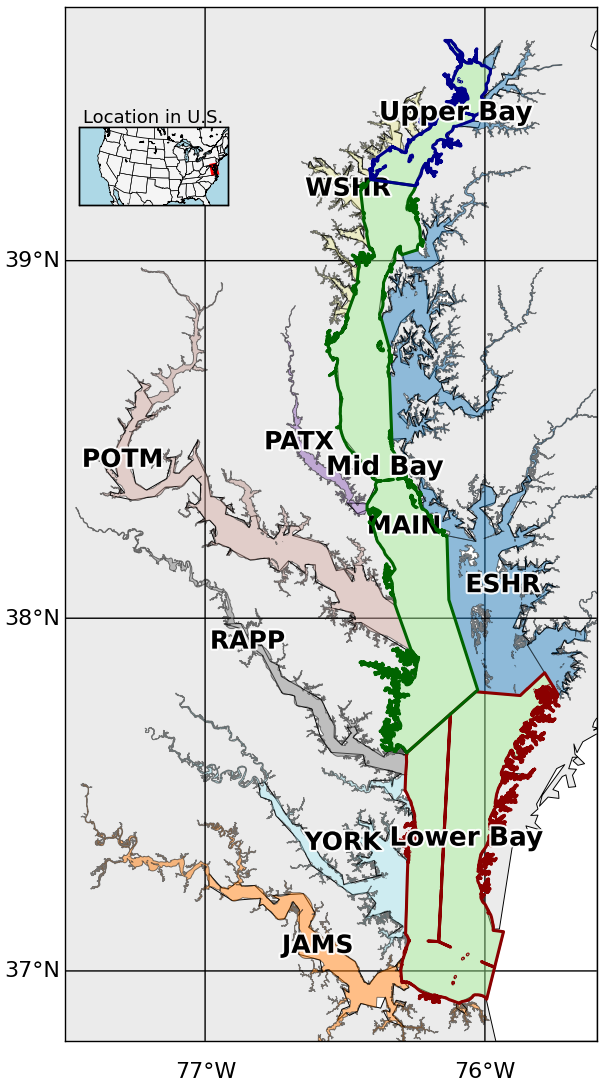
Figure 1 Segmentation of the mainstem of the Chesapeake Bay and its tidal tributaries. The mainstem is divided into three regions, Upper Bay, Mid Bay, and Lower Bay. Acronyms denote specific tributaries and sub-estuarine areas: ESHR refers to Eastern Shore tributaries, WSHR to Western Shore tributaries, POTM to the Potomac River, PATX to the Patuxent River, RAPP to the Rappahannock River, YORK to the York River system (including the Mattaponi and Pamunkey Rivers), and JAMS to the James River.

In our study, we build on this previous work by addressing the following research questions in the context of the Chesapeake Bay:

1. To what extent do benthic macrofauna contribute to estuarine carbon cycling through respiration and calcification, and how might these contributions vary across space?

2. How well can environmental variables routinely collected in estuarine monitoring programs predict benthic macrofauna biomass?

Answering these questions will help clarify the role of benthic macrofauna in estuarine carbon cycling and improve the ability of monitoring programs and numerical models to account for benthic processes using more accessible environmental data.

2 Methods

2.1 Overview

We examined historic benthic macrofauna biomass data collected annually by the Chesapeake Bay Long-Term Benthic Monitoring Program (BMP) (Dauer et al., 2000; Llansó and Zaveta, 2017). We applied empirical relationships linking biomass to secondary production, respiration, and calcification to quantify the impact of benthic macrofauna on carbon cycling in the Bay. To identify environmental predictors of benthic biomass, we compiled measurements of bottom water temperature, salinity, dissolved oxygen, and sediment sand fraction measured by the BMP at the same time and location as the benthic biomass samples. In addition to these measured environmental variables, we utilized output from ROMS-ECB, which is a three-dimensional estuarine carbon and biogeochemistry (ECB) model embedded into the Regional Ocean Modeling System (ROMS; Shchepetkin and McWilliams, 2005) developed for the Chesapeake Bay (St-Laurent and Friedrichs, 2024b). We identified correlations between these environmental variables (observed and modeled) and benthic macrofauna biomass using generalized additive models (GAMs).

2.2 Benthic biomass data

Details of the BMP data we used in our study are described elsewhere (Dauer, 1993; Dauer et al., 2000; Dauer and Lane, 2010; Llansó and Scott, 2011; Llansó and Zaveta, 2017) and are summarized here. The program began in 1984, but consistency in sampling started in 1995. The sampling occurs mainly in the summer, between 15 July and 30 September, at both fixed and random stations, with the latter changing location every year. The sampling is conducted separately by the states of Maryland (Llansó and Zaveta, 2017) and Virginia (Dauer and Lane, 2010), with slightly different protocols used in each state (see below). Our analysis spanned 1995 to 2022, the recent extent of available data, incorporating 28 years of data.

The Maryland monitoring program comprises 27 fixed and 150 random stations in the upper Chesapeake Bay. The Virginia monitoring program comprises 21 fixed and 100 random stations in the lower Chesapeake Bay. In Virginia, random stations were not sampled in 1995, and fixed stations were not sampled in 2017 or 2018. Water depths greater than 12 m in the mainstem part of the Bay in Maryland are not sampled because the bottom waters become anoxic in the summer, resulting in azoic sediments. The tributaries are sampled only in the tidal zone; areas with less than 1 m mean lower low water are considered non-tidal. Some locations, such as oyster reefs and other hard substrates, are also not sampled due to gear unsuitability in such habitats. To avoid seasonal biases, we excluded samples collected outside of the summer sampling window of 15 July–30 September, which occurred earlier in the study period. This selection resulted in a dataset of 8128 samples across both states, or an average of 290 samples per year, slightly less than the maximum of 298.

At each sampling station, the uppermost layers of sediment are collected. In Maryland, the sites introduced in 1995 (two fixed sites and all random sites) are sampled with a Young grab, which collects a surface area of 0.0440 m² to a depth of 0.10 m. For the other fixed sites in Maryland, nearshore shallow sandy habitats of the mainstem and tributaries are sampled with a modified box corer with a surface area of 0.0250 m² to a depth of 0.25 m. Muddy habitats and deep-water habitats in the mainstem and tributaries of Maryland are sampled with a Wildco box corer with a surface area of 0.0225 m² to a depth of 0.23 m. The fixed site in the Nanticoke River is sampled with a Petite Ponar grab with a surface area of 0.0250 m² to a depth of 0.07 m. In Virginia, fixed sites use a spade-type box-coring device with a surface area of 0.0182 m² to a depth of 0.02 m; random sites use a Young grab with a surface area of 0.0400 m² to a depth of 0.10 m. One limitation of using multiple types of sampling gear is that differences in design, such as penetration depth, sample volume, and sediment disturbance, can introduce variability in estimates of benthic diversity, abundance, and biomass (Eleftheriou and Moore, 2013).

For both monitoring programs, the sampling contents are sieved through a 0.5 mm screen to retain only benthic macrofauna. The macrofauna are identified at the lowest taxonomical level. The specimens are dried on a pan for at least 24 h to a constant weight, then a final weight is measured. The specimens are then placed in a muffle furnace for 4 h at 500 °C for ashing, and the specimens are weighed again. The ash-free dry weight (AFDW), representing only the soft-tissue biomass, is the difference between the dry and ashed weight. We converted the AFDW in g per sample to biomass density B in units of g m⁻² by dividing the AFDW by the area of the sampling device. The data used in our subsequent statistical analysis include the biomass density of individually selected species and classes and the total biomass density.

Benthic biomass is known to be highly patchy, with large variability even between samples taken in close proximity, hence the common use of replicate sampling in field protocols. To mitigate this noise and extract meaningful large-scale spatial patterns, we averaged across the 28-year time frame. All 8128 biomass samples collected from 1995 to 2022 were averaged onto a uniform grid with cells each measuring 0.04° in longitude and 0.03125° in latitude (∼ 3.5 km per side). 1295 cells had at least one biomass measurement during the 28-year period. Across these cells, the average number of samples was 6.19, the median was 3, and the maximum was 69. Tributaries and the upper Bay were sampled more densely than the mainstem (Appendix A and Fig. A1). This “time-averaging” approach enabled clearer interpretation of spatial gradients in biomass and strengthened the robustness of subsequent statistical analyses aimed at identifying consistent environmental drivers. Some benthic biomass sampling stations fell outside the Chesapeake Bay Program (CBP) water quality segmentation scheme, which was originally developed to support monitoring and management analyses (Anon, 2004). The CBP segments are defined at a relatively coarse spatial scale and often exclude narrow nearshore environments and small tributary creeks. To maintain consistency with the spatial framework used in coupled hydrodynamic–biogeochemical models, in our case ROMS-ECB, we excluded these points from analysis. This filtering step ensured that all biomass observations were aligned with the modeled domain, avoiding mismatches at the land–water interface. After this step, 1008 grid cells remained, of which 868 contained at least one biomass observation and the remainder were empty cells.

2.3 Carbon flux estimations

To estimate the impact of benthic macrofauna on carbon cycling, we applied empirical equations from the literature to quantify secondary production, calcification, and respiration. These equations were identified through an informal literature review using online tools (e.g., Google Scholar), with emphasis on studies relevant to soft-sediment bivalves, the dominant macrofauna in the Chesapeake Bay. We prioritized relationships applicable to local taxa and easily scalable to our biomass dataset. While multiple sources were available for secondary production, equations for respiration and calcification were more limited; in those cases, we selected models based on representative species that could be scaled from production estimates. We used a range of published values for biomass-to-carbon conversion, secondary production, and species-specific respiration and calcification ratios to estimate upper and lower bounds of carbon fluxes. Additional details on uncertainty calculations are provided in the Appendix B.

2.3.1 Secondary production

We converted biomass to secondary production S (units of g C m⁻² yr⁻¹). Multiple approaches have been used for this conversion, and we used the average of three approaches to be able to broadly quantify uncertainty in our estimates.

In the first approach, secondary production is given by:

$$\begin{array}{}\text{(5)}& S_{\mathrm{1}}=\mathit{\alpha }{B}_{\mathrm{c}}\end{array}$$

where α is the specific growth rate and B_c is carbon-based biomass (units of g C m⁻²). We found three studies that estimated α for benthic macrofauna. At the low end, a study of benthic macrofauna in the Chesapeake Bay used α=1.06 yr⁻¹ (Wilson and Fleeger, 2023). At the high end, a study of C. fluminea used α=4.45 yr⁻¹ (Chauvaud et al., 2003). An intermediate value of α=2 yr⁻¹ was based on monthly observations of benthic macrofauna dominated by the crustacean Corophium volutator and the bivalve Limecola balthica at an intertidal site in the upper Bay of Fundy (Schwinghamer et al., 1986). A mean value of 2.50 yr⁻¹ was used in Eq. (5). B_c is computed from biomass B (units of g m⁻²) using:

$$\begin{array}{}\text{(6)}& B_{\mathrm{c}}=r_{\mathrm{c}}B\end{array}$$

where r_c is the ratio of carbon mass to total mass in benthic organic matter. In a study on the bivalve filter feeders Rangia cuneata and Corbicula fluminea, which dominate in the tidal fresh and oligohaline waters of the Chesapeake Bay, r_c=0.47 g C g⁻¹ was used (Cerco and Noel, 2010). A slightly lower value of 0.41 g C g⁻¹ was used in a study of native and introduced bivalves in six North American freshwater systems (Chauvaud et al., 2003). A mean value of r_c=0.44 g C g⁻¹ was used in our calculation.

In the second approach, temperature (T) dependence for bivalve secondary production was added (Sturdivant et al., 2013):

$$\begin{array}{}\text{(7)}& S_{\mathrm{2}}=S_{\mathrm{0}}{\left({\displaystyle \frac{B}{\mathrm{1}\mathrm{g}{\mathrm{m}}^{-\mathrm{2}}}}\right)}^{\mathrm{0.87}}{\left({\displaystyle \frac{T}{\mathrm{1}{}^{\mathrm{o}}\mathrm{C}}}\right)}^{\mathrm{0.46}}\end{array}$$

where S₀=0.40 g C m⁻² yr⁻¹. Note that the coefficient at the beginning of the equation differs from that of Sturdivant et al. (2013) because of a change in units of B from mg to g m⁻² and of S from mg C d⁻¹ to g C m⁻² yr⁻¹. This equation has been shown to agree well with secondary production and biomass measurements (Sturdivant et al., 2013).

Finally, in the third approach (Tumbiolo and Downing, 1994), depth (Z) dependence was added:

$$\begin{array}{}\text{(8)}& \begin{array}{rl}{\log }_{\mathrm{10}}& \left({\displaystyle \frac{S_{\mathrm{3}}}{\mathrm{1}\mathrm{g}\mathrm{C}{\mathrm{m}}^{-\mathrm{2}}{\mathrm{yr}}^{-\mathrm{1}}}}\right)={\mathit{\beta }}_{\mathrm{0}}+b{\log }_{\mathrm{10}}\left({\displaystyle \frac{B}{\mathrm{1}\mathrm{g}{\mathrm{m}}^{-\mathrm{2}}}}\right)\\ & -m{\log }_{\mathrm{10}}\left({\displaystyle \frac{M}{\mathrm{1}\mathrm{mg}}}\right)+t\left({\displaystyle \frac{T}{\mathrm{1}{}^{\mathrm{o}}\mathrm{C}}}\right)\\ & -z{\log }_{\mathrm{10}}\left({\displaystyle \frac{Z}{\mathrm{1}\mathrm{m}}}+\mathrm{1}\right)\end{array}\end{array}$$

where β₀=0.24, b=0.96, m=0.21, t=0.03, =0.16, and M is the maximum individual body mass. Eq. 8 was developed by Tumbiolo and Downing (1994) through multiple regression analysis of 125 benthic invertebrate populations, including data from the Chesapeake Bay. In their model, M refers to the maximum individual mass of the largest size class observed within a population. It was identified as the second most important predictor of secondary production after total biomass. Their analysis showed that species with greater maximum sizes tend to have slower turnover rates and lower production-to-biomass ratios. In our application, we treated M as a constant, based on the maximum individual mass of the bivalve R. cuneata collected in a study in the Choptank River in the Chesapeake Bay, which was 5953 mg (Hartwell et al., 1991). R. cuneata is among the most abundant and largest benthic macrofaunal species in our study area (Cerco and Noel, 2010; Hartwell et al., 1991).

In Eqs. (7) and (8), we used the bottom water temperature measured on the same day the benthic samples were collected. This reliance on summer temperature values represents a key limitation of our study, as it likely leads to overestimation of annual secondary production, particularly for Eq. (8). For example, Eqs. (7) and (8) both predict maximum summer secondary production that is about 5 times larger than the minimum winter production, assuming an annual temperature range of 1 to 25 °C. However, we note that the first approach for secondary production (Eq. 6) has no temperature dependence. Figures C1–C3 in Appendix C provide a detailed comparison of secondary production across the three models and assess temperature effects on Models 2 and 3.

2.3.2 Calcification

Benthic macrofaunal calcification C (g CaCO₃ m⁻² yr⁻¹) was computed from secondary production following Chauvaud et al. (2003):

$$\begin{array}{}\text{(9)}& C=r_{\mathrm{s}}S\end{array}$$

where r_s is the ratio of shell CaCO₃ mass production to tissue organic C mass production, which has units of g CaCO₃ (g C⁻¹). Based on samples of the bivalve Potamocorbula amurensis in the northern San Francisco Bay, Chauvaud et al. (2003) found r_s to be 10 g CaCO₃ (g C⁻¹). They also cited a ratio of 15 g CaCO₃ (g C⁻¹) for the bivalve C. fluminea, a more relevant species to our study, but the reference is from unpublished data. We used the average of the two values, 12.5 g CaCO₃ (g C⁻¹), which corresponds to a molar ratio of 1.5 mol CaCO₃ (mol C⁻¹).

2.3.3 Respiration

The ratio of respiration to secondary production, expressed as energy fluxes, was derived from an empirical relationship between benthic macrofauna biomass and respiration in the Bay-of-Fundy study referenced earlier (Schwinghamer et al., 1986):

$$\begin{array}{}\text{(10)}& {\log }_{\mathrm{10}}\left({\displaystyle \frac{R}{\mathrm{1}\mathrm{kcal}{\mathrm{m}}^{-\mathrm{2}}{\mathrm{yr}}^{-\mathrm{1}}}}\right)={\mathit{\alpha }}_{\mathrm{0}}+s{\log }_{\mathrm{10}}\left({\displaystyle \frac{S}{\mathrm{1}\mathrm{kcal}{\mathrm{m}}^{-\mathrm{2}}{\mathrm{yr}}^{-\mathrm{1}}}}\right)\end{array}$$

where s=0.993 and α₀=0.367. Since s is nearly 1, the relationship simplifies to:

$$\begin{array}{}\text{(11)}& R={\mathrm{10}}^{{\mathit{\alpha }}_{\mathrm{0}}}S=\mathrm{2.33}S\end{array}$$

Assuming that the conversion between carbon and energy is the same for S and R, this equation can be directly applied to these processes expressed as carbon fluxes, consistent with our other carbon flux estimates. Further, combining the relationships of calcification and respiration with secondary production on a molar basis allows a best estimate of the molar ratio of respiration to calcification: $\mathrm{2.33}/\mathrm{1.5}=\mathrm{1.55}$.

2.3.4 Impact on the carbonate system

From the estimated benthic macrofaunal calcification (C) and respiration (R), we calculated TA and DIC fluxes (units of mol m⁻² yr⁻¹):

$$\begin{array}{}\text{(12)}& {\displaystyle }{F}_{\mathrm{TA}}={\displaystyle \frac{-\mathrm{2}C}{M_{{\mathrm{CaCO}}_{\mathrm{3}}}}}\text{(13)}& {\displaystyle }{F}_{\mathrm{DIC}}={\displaystyle \frac{R}{M_{\mathrm{C}}}}-{\displaystyle \frac{C}{M_{{\mathrm{CaCO}}_{\mathrm{3}}}}}\end{array}$$

where $M_{{\mathrm{CaCO}}_{\mathrm{3}}}$ and M_C are the molar masses of CaCO₃ and C, respectively, and the sign convention is positive from the benthic fauna to the water column. Both calcification and respiration will lead to increases in the concentration of aqueous CO₂, and so there is a CO₂ flux from benthic fauna that can be decomposed into CO₂ fluxes resulting from these two processes:

$$\begin{array}{}\text{(14)}& F_{{\mathrm{CO}}_{\mathrm{2}}}=F_{{\mathrm{CO}}_{\mathrm{2}}}^{\mathrm{TA}}+F_{{\mathrm{CO}}_{\mathrm{2}}}^{\mathrm{DIC}}\end{array}$$

It has been estimated, assuming air–sea CO₂ equilibrium, that every mole of CaCO₃ precipitated leads to the evasion of 0.6–1 mole of CO₂ to the atmosphere, depending on the temperature, salinity, atmospheric pCO₂, and initial alkalinity (Chauvaud et al., 2003; Frankignoulle et al., 1998; Ware et al., 1992).

In light of strong departures from air–sea CO₂ equilibrium in estuaries, including the Chesapeake Bay (Herrmann et al., 2020), we instead estimate the production rate of CO₂ using buffer factors, ζ_TA and ζ_DIC, which are defined as the fractional change in [CO₂] divided by the fractional change in [TA] and [DIC], respectively; e.g., ${\mathit{\zeta }}_{\mathrm{TA}}=\left(\mathrm{\Delta }\right[{\mathrm{CO}}_{\mathrm{2}}]/[{\mathrm{CO}}_{\mathrm{2}}\left]\right)/\left(\mathrm{\Delta }\right[\mathrm{TA}]/[\mathrm{TA}\left]\right)$. This approach also allows us to estimate the CO₂ flux from respiration. We computed the buffer factors in three steps. First, we used output from ROMS-ECB (described in more detail later in the Methods Sect. 2.4) for the years 1995–2022 and calculated long-term averages of bottom [TA], [DIC], temperature, salinity, and pressure (estimated from water depth) at each model grid cell. These values were used as input to PyCO₂SYS (Humphreys et al., 2022) to calculate the baseline [CO₂]. Second, we individually perturbed [TA] and [DIC] by 1 % (Δ[TA] and Δ[DIC]) while holding all other variables constant and recalculated [CO₂] to get Δ[CO₂]. Third, we computed ζ_TA and ζ_DIC using the definition of the buffer factors.

To relate the fluxes to the buffer factors, we use the flux form of the buffer factors:

$$\begin{array}{}\text{(15)}& {\displaystyle }{\mathit{\zeta }}_{\mathrm{TA}}={\displaystyle \frac{F_{{\mathrm{CO}}_{\mathrm{2}}}^{\mathrm{TA}}/\left[{\mathrm{CO}}_{\mathrm{2}}\right]}{F_{\mathrm{TA}}/\left[\mathrm{TA}\right]}}\text{(16)}& {\displaystyle }{\mathit{\zeta }}_{\mathrm{DIC}}={\displaystyle \frac{F_{{\mathrm{CO}}_{\mathrm{2}}}^{\mathrm{DIC}}/\left[{\mathrm{CO}}_{\mathrm{2}}\right]}{F_{\mathrm{DIC}}/\left[\mathrm{DIC}\right]}}\end{array}$$

These flux forms take the definitions of the buffer factors and replace ratios of concentration changes (e.g., $\mathrm{\Delta }\left[{\mathrm{CO}}_{\mathrm{2}}\right]/\mathrm{\Delta }\left[\mathrm{TA}\right]$) with ratios of fluxes (e.g., $F_{{\mathrm{CO}}_{\mathrm{2}}}/F_{{\mathrm{CO}}_{\mathrm{2}}}^{\mathrm{TA}}$). Using Eqs. (15) and (16) in Eq. (14) yields an expression for the CO₂ flux from benthic fauna to the water column:

$$\begin{array}{}\text{(17)}& F_{{\mathrm{CO}}_{\mathrm{2}}}=\left[{\mathrm{CO}}_{\mathrm{2}}\right]\left({\displaystyle \frac{{\mathit{\zeta }}_{\mathrm{TA}}{F}_{\mathrm{TA}}}{\left[\mathrm{TA}\right]}}+{\displaystyle \frac{{\mathit{\zeta }}_{\mathrm{DIC}}{F}_{\mathrm{DIC}}}{\left[\mathrm{DIC}\right]}}\right)\end{array}$$

2.3.5 Spatial analysis and comparison to other carbon fluxes

To place benthic macrofauna contributions to estuarine carbon cycling in a broader spatial context, we averaged fluxes over 10 regions based on aggregated Chesapeake Bay Program segments (Fig. 1): the major tidal tributaries (the Patuxent, Potomac, Rappahannock, York, and James River Estuaries), the Western and Eastern Shores, and the Upper, Mid, and Lower (mainstem) Bay. Additionally, we computed averages over the mainstem Bay and the whole Bay. For each region, we calculated benthic respiration and bivalve calcification rates based on observed biomass, using the empirically derived equations just described. We then compared these fluxes to other components of the estuarine carbon budget using published values for primary production, allochthonous organic carbon inputs, oyster calcification, and air–sea gas exchange.

First, we assessed the extent to which benthic macrofauna remineralize organic carbon inputs by comparing our calculated respiration rates to net primary production (NPP) and external particulate organic carbon (POC) loads. Primary production and POC values were obtained from prior studies (Herrmann et al., 2015; Kemp et al., 1997; Najjar et al., 2018; Zhang and Blomquist, 2018) and scaled to match the spatial extent of our biomass data. In the Upper Bay, we calculated organic carbon inputs by distributing the Susquehanna River's POC load over the combined surface area of the oligohaline and tidal fresh segments (CB1 and CB2; Olson, 2012). This approach assumes that the majority of the annual POC load from the Susquehanna River remains concentrated in the Upper Bay and is respired rather than transported downstream, an assumption supported by Canuel and Hardison (2016). For comparison, we also distributed Susquehanna River POC inputs across the entire mainstem. For brevity, we restricted our tributary-level comparison to the Potomac River Estuary, where the full organic carbon load was distributed across the surface area of the entire tidal tributary (Fig. 1).

Second, we compared our soft-sediment bivalve calcification estimates to published oyster calcification rates from Fulford et al. (2007). Oyster ash-free dry weight was converted to live weight using a 10:1 ratio (Mo and Neilson, 1994), and a calcification rate of 2 mg CaCO₃ per g⁻¹ live weight per day was applied (Waldbusser et al., 2013). Because Eastern oyster (Crassostrea virginica) populations in the Chesapeake Bay were historically at least two orders of magnitude higher than current levels (Fulford et al., 2007; Newell, 1988), we also scaled published oyster calcification rates up by a factor of 100 to estimate potential historical contributions. This comparison allowed us to place present-day bivalve calcification into the broader context of ecosystem function.

Third, we evaluated whether riverine calcium supply could limit observed calcification by estimating annual calcium fluxes from the Susquehanna and Potomac Rivers using non-tidal USGS data from 1995 to 2022 and the Weighted Regression on Time, Discharge, and Season (WRTDS) method (Hirsch et al., 2010). Assuming a 1:1 molar ratio between Ca²⁺ and CaCO₃ formation, we estimated the maximum potential calcification that could occur if all incoming calcium were used for shell production in adjacent estuarine zones.

Finally, we compared CO₂ generated from respiration and calcification (Eq. 17) to published estimates of air–sea CO₂ exchange (Chen et al., 2013; Herrmann et al., 2020).

The estimated carbon fluxes reveal important spatial patterns, but their interpretation should be tempered by uncertainty in several underlying assumptions. While secondary production models are relatively well-calibrated across estuarine systems, the calculations for calcification and respiration are more sparse and less empirically constrained. Our propagated uncertainty in calcification and respiration incorporates variation in biomass-based carbon content, multiple conversion approaches from biomass to secondary production, and calcification parameters derived from two different bivalve species. Although we used different methods to estimate calcification and propagated these uncertainties accordingly, only one approach was available for respiration.

We estimated uncertainties in F_DIC and F_TA, which represent the propagated uncertainties from respiration and calcification alone, with no additional sources of uncertainty included in those calculations. However, we did not calculate formal uncertainties in $F_{{\mathrm{CO}}_{\mathrm{2}}}$ due to the complexity involved. Additional uncertainty in $F_{{\mathrm{CO}}_{\mathrm{2}}}$ arises from the use of annually averaged, model-derived values for salinity, temperature, depth, DIC, and TA. Further uncertainty stems from the method used to calculate ζ from TA and DIC perturbations. While these additional sources contribute to the overall uncertainty in $F_{{\mathrm{CO}}_{\mathrm{2}}}$, the uncertainties in F_DIC and F_TA are likely to remain the dominant contributors.

The resulting error bars in the various carbon fluxes reflect these methodological uncertainties, offering a plausible range rather than precise values. Thus, the benthic macrofaunal carbon fluxes presented here should be interpreted with some caution, with more confidence given to the broad spatial patterns and less to the absolute values.

2.4 Environmental predictors of benthic biomass

From the BMP, we used bottom temperature, salinity, and dissolved oxygen data, which are measured with a YSI 660 Sonde or Hydrolab DataSonde 4a in Maryland and a YSI 85 Model meter in Virginia 1 m above the sediment surface. Extreme outliers, defined as data points that fall beyond three times the interquartile range from the first or third quartile, were removed. As a result, one value for dissolved oxygen and one for water temperature were excluded from the analysis. The salinity zones are also characterized at each site as tidal fresh (<0.5 ppt), oligohaline (0.5–5 ppt), low mesohaline (5–12 ppt), high mesohaline (12–18 ppt), and polyhaline (>18 ppt); these zones are relatively geographically fixed (with some changes in 2011 due to Hurricane Irene and Tropical Storm Lee) based on long-term averages of salinity (Llansó, 2002; Llansó and Zaveta, 2017). Sediment sand fraction was measured by first collecting two 120 mL benthic grab sub-samples. Sand particles are separated by wet-sieving through a 63 µm stainless steel sieve. Sand fraction is recorded after drying and weighing the samples. The bottom water quality and sediment composition data were time-averaged using the same scheme described earlier for the benthic biomass data.

ROMS-ECB output was used to characterize environmental variables not measured by the BMP that could be relevant to predicting the benthic macrofauna biomass distribution. ROMS-ECB uses 20 terrain-following vertical levels and a uniform horizontal resolution of 600 m (St-Laurent and Friedrichs, 2024b). We compiled daily averaged output at various grid points from 1995 to 2022 corresponding to the locations of each of the 8128 benthic biomass samples. We selected the ROMS output at the nearest ROMS grid point to each BMP sample location for each variable of interest, described below. Several ROMS-ECB environmental variables are directly linked to primary production, but the timing of peak primary production does not always align with periods of greatest food availability for benthic organisms. To capture ecologically meaningful variation in benthic–pelagic coupling, we calculated both seasonal and annual averages for each variable. Seasonal groupings reflect key ecological periods: spring (March–May), which includes the diatom bloom that delivers fresh organic material to the benthos, and summer (June–August), characterized by stratification, hypoxia, and intense remineralization. Fall (September–November) and winter (December–February) were also included to represent background seasonal variability. We then time-averaged the seasonal and annual means as described earlier. Coverage dropped from 868 to 846 cells after adding ROMS-ECB outputs, largely where the model masks shallow/tributary cells or lacks complete seasonal data.

We used ROMS-ECB output, as opposed to data from the Chesapeake Bay Water Quality Monitoring Program (WQMP), which has measured water quality variables since 1984 at over 100 tidal stations (Chesapeake Bay Program, 2004). The WQMP stations are at different locations than the BMP stations, requiring interpolation to correlate these data with benthic biomass. Other studies have opted to use kriging, a method used to spatially interpolate surface water quality data, to increase the spatial resolution. Kriging has been found to outperform the standard inverse distance weighting tools typically used in the Chesapeake Bay (Murphy et al., 2015). One study evaluated the kriging of surface WQMP data for July 2007 using 117–123 data points (Murphy et al., 2015). In cross-validation, one measured sample is removed, and the interpolation is then performed at that location; the interpolated value is then compared to the observed value. Cross-validation of temperature, salinity, and dissolved oxygen yielded root-mean-square errors (RMSE) of 0.75 °C, 1.1 ppt, and 1.2 mg L⁻¹, respectively. In contrast, ROMS-ECB output was evaluated with over 500 000 WQMP data points at multiple depths and locations from 1985 to 2021 (St-Laurent and Friedrichs, 2024a). The RMSEs for temperature, salinity, and dissolved oxygen were 1 °C, 1.9 psu, and 1.5 mg L⁻¹, respectively. Although these RMSEs are slightly higher than those from kriging, the evaluation was much more robust, and the long time series evaluation is more relevant to our time-averaging technique over 28 years. In addition, we wanted to utilize bottom water quality data, as these variables are measured closer to the location of benthic macrofauna. However, cross-validation for kriging was only performed at the surface (Murphy et al., 2015), possibly due to the challenges of accounting for bottom topography in spatial interpolation.

ROMS-ECB simulates many variables, and we considered the subset that might be good predictors of benthic biomass: bottom POC, bottom total suspended solids (TSS), and surface NO${}_{\mathrm{3}}^{-}$. POC was considered because a large fraction of POC represents food for benthic macrofauna. TSS was considered a metric of suspended inorganic material, which can inhibit filter-feeding organisms (Grant and Thorpe, 1991). Photosynthesis is largely limited by NO${}_{\mathrm{3}}^{-}$ in the Chesapeake Bay (Zhang et al., 2021); because phytoplankton productivity and the subsequent sinking of POC is an important source of organic matter to the benthos, NO${}_{\mathrm{3}}^{-}$ could be a predictor of benthic biomass. ROMS-ECB output was evaluated for robustness with WQMP data using Spearman's rank correlation coefficient, R_s, which measures the strength of the association between two variables (Hauke and Kossowski, 2011). In our analysis of benthic biomass predictors, we included only variables with R_s above 0.7, which generally indicates a strong association (Akoglu, 2018). NO${}_{\mathrm{3}}^{-}$ was used as it had R_s=0.77, whereas POC and TSS were not as they had R_s=0.26 and 0.24, respectively (St-Laurent and Friedrichs, 2024a).

We also considered potentially good predictors that could be computed from ROMS-ECB output: surface oxygen supersaturation (ΔO₂) and bottom aragonite saturation state (Ω_arag). ΔO₂ can be used as a tracer for net ecosystem production (Herrmann et al., 2020) and hence may indicate organic matter availability to the benthos. Δ[O₂] is equal to O₂ minus the saturation concentration, which was computed from temperature and salinity (Garcia and Gordon, 1992). Positive ΔO₂ values are favored during net autotrophy (photosynthesis exceeds respiration), while negative values are favored during net heterotrophy (respiration exceeds photosynthesis); temperature change and transport can also create non-zero ΔO₂. Ω_arag could predict benthic biomass because bivalve calcification is expected to depend on this metric (Thomsen et al., 2015). PyCO₂SYS (Humphreys et al., 2022) was used to derive the solubility product and carbonate ion concentration from alkalinity, DIC, temperature, salinity, and water depth. We examined ΔO₂ and Ω_arag in the subsequent statistical analysis because the ROMS-ECB output variables used to compute them all had R_s>0.7. Although calcium measurements were not available for model evaluation, it is highly correlated to salinity, though deviations may occur at low salinity (Beckwith et al., 2019).

2.5 Statistical modeling of benthic biomass

We used GAMs to evaluate how bottom water quality and biogeochemical model outputs predict the spatial distribution of benthic macrofaunal biomass. GAMs are data-driven statistical models that have been widely applied in coastal ecology since the late 20th century (Guisan et al., 2002; Smith et al., 2023). They model additive, smoothed relationships between predictor and response variables, making them well-suited for capturing the non-linear, non-monotonic patterns often observed in ecological datasets (Grüss et al., 2014; Guisan et al., 2002; Hastie and Tibshirani, 1987; Wood, 2017). GAMs also quantify the strength and relative contribution of each predictor (Guisan et al., 2002) and have demonstrated predictive performance comparable to or exceeding other modeling approaches (Drexler and Ainsworth, 2013). We used the mgcv package in R and applied restricted maximum likelihood (REML) to optimize smoothness (Wood, 2011, 2017). This approach is particularly effective with large datasets like ours, enabling robust estimation of spatial patterns in biomass across a broad geographic region (Grüss et al., 2014; Wood, 2011). Although GAMs can handle non-normal distributions of the response variable (Guisan et al., 2002), we found the best model fit by applying a natural logarithmic transformation to the biomass. A small constant (0.0001 g m⁻²) was added to the biomass values before applying the natural logarithmic transformation to account for zeros in the data.

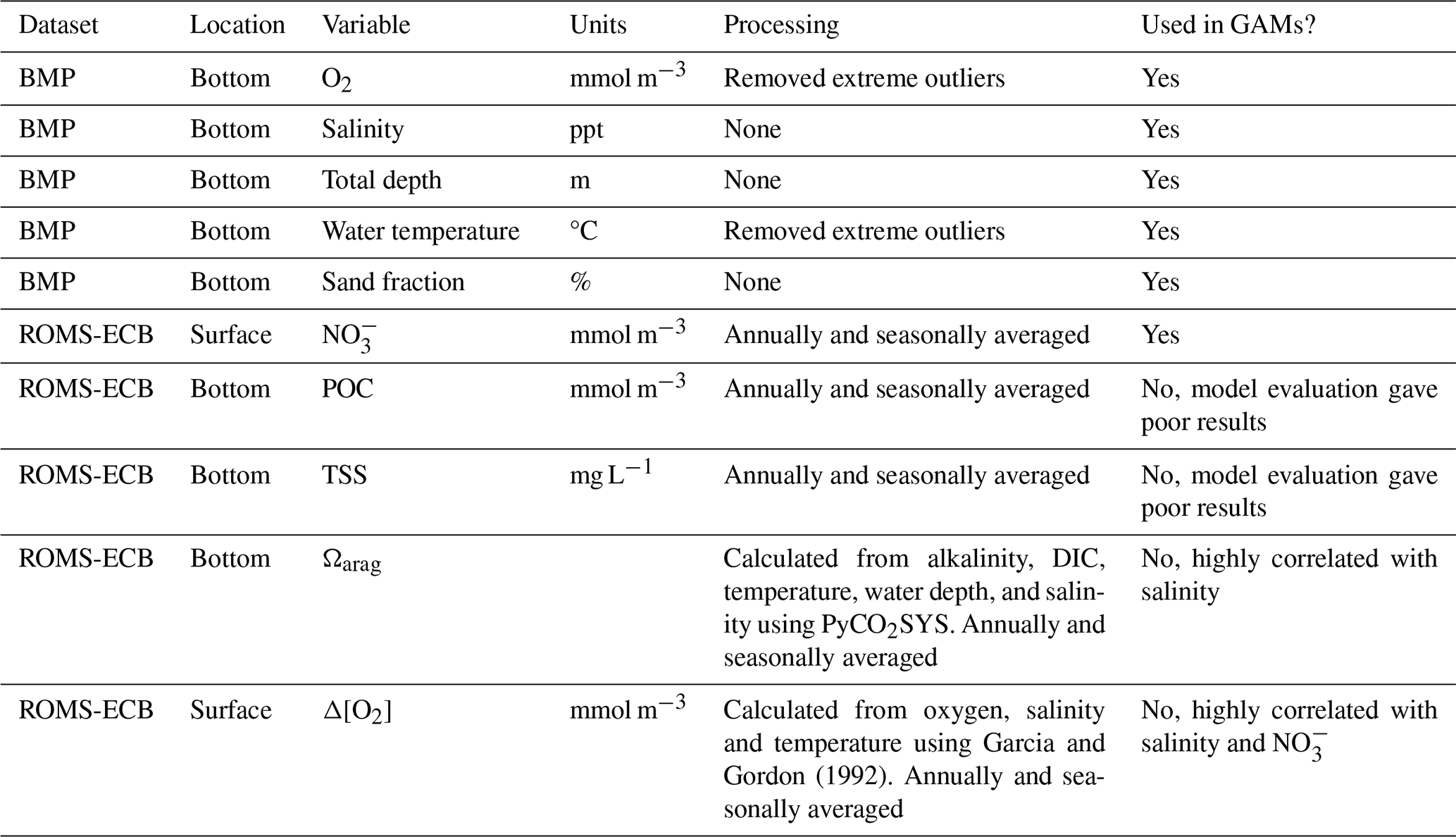
As described earlier, we initially identified eight environmental variables: O₂, salinity, total depth, water temperature, sand fraction, NO${}_{\mathrm{3}}^{-}$, Ω_arag, and Δ[O₂]. To avoid multicollinearity, which can distort GAM results (Grüss et al., 2014; Grüss et al., 2018; Guisan et al., 2002), we used Pearson's correlation coefficients (r) to evaluate the linear correlation between the predictor variables. When two variables were highly correlated (r>0.7) (Dormann et al., 2013), we retained the variable that was more directly measurable and broadly understood across estuarine systems. Based on this assessment, we excluded Ω_arag and Δ[O₂] due to their strong correlation with other variables and retained the remaining six variables for GAM analysis. While necessary for model stability, this approach may limit the explanatory power of the GAM by excluding ecologically meaningful predictors. The full list of candidate variables and their inclusion status is provided in Table 1.

Table 1 Predictor variables from the Chesapeake Bay Benthic Monitoring Program and ROMS-ECB compiled from 1995–2002. For ROMS-ECB output, daily values were used to calculate annual averages and seasonal averages for spring (March–April), summer (July–August), fall (September–November), and winter (December–February).

We used Akaike's Information Criterion (AIC), a statistical measure that has been increasingly used in ecology, to evaluate which combination of parameters results in the best model fit (Symonds and Moussalli, 2011). AIC is calculated using the number of fitted parameters in the model, the maximum likelihood estimate, and the residual sum of squares (Symonds and Moussalli, 2011). Among the candidate models, the one with the lowest AIC value offers the best balance between explanatory power and simplicity, requiring the fewest necessary parameters. We chose the assemblage of predictor variables in our model that minimized AIC. We generally used annually averaged predictor variables from the ROMS-ECB output because using seasonal averages had a negligible difference on the AIC. To assess the relative influence of each predictor variable, we used Akaike weights, which indicate the probability that a given model is the best among those considered. We ranked models by AIC and summed the Akaike weights for all models containing each predictor variable. Higher Akaike weights indicate stronger support for a variable's inclusion in the best-fitting models. Interaction terms between predictor variables were examined, but their inclusion did not significantly improve the AIC values.

3 Results

3.1 Spatial distribution of benthic macrofauna biomass

The time-averaged (1995–2022) summer benthic macrofauna biomass exhibits strong spatial variability across the Chesapeake Bay, with higher concentrations in the tidal fresh and oligohaline zones, and lower concentrations in the Mid Bay and lower sections of many tributaries (Figs. 2, 3a). The arithmetic mean of all biomass measurements based on the full data set, N=8128 is 7.93 g m⁻² (median = 0.98 g m⁻²), whereas the spatial mean across all grid cells with at least one biomass measurement (N=1295) is 7.16 g m⁻² (median = 1.39 g m⁻²). The sampling scheme oversamples the tidal tributaries (Fig. A1), where biomass density is higher, inflating the arithmetic mean. The standard deviation of the full dataset is 28.7 g m⁻², indicating that the distribution is heavily skewed to the right, with the highest sample reaching up to 722 g m⁻². The standard deviation of the time-averaged data is 18.0 g m⁻², considerably smaller than the full data set since it does not include temporal variability, but is nevertheless still skewed to the right, with the highest gridded value of 220 g m⁻². Most of the high-biomass density zones (>30 g m⁻²) are concentrated in the tidal fresh and oligohaline sections of the mainstem and Potomac River Estuary. The other tributaries have higher biomass in the tidal fresh and oligohaline and zones compared to the other salinity zones. In the Mid Bay and lower sections of many tributaries, biomass is very low.

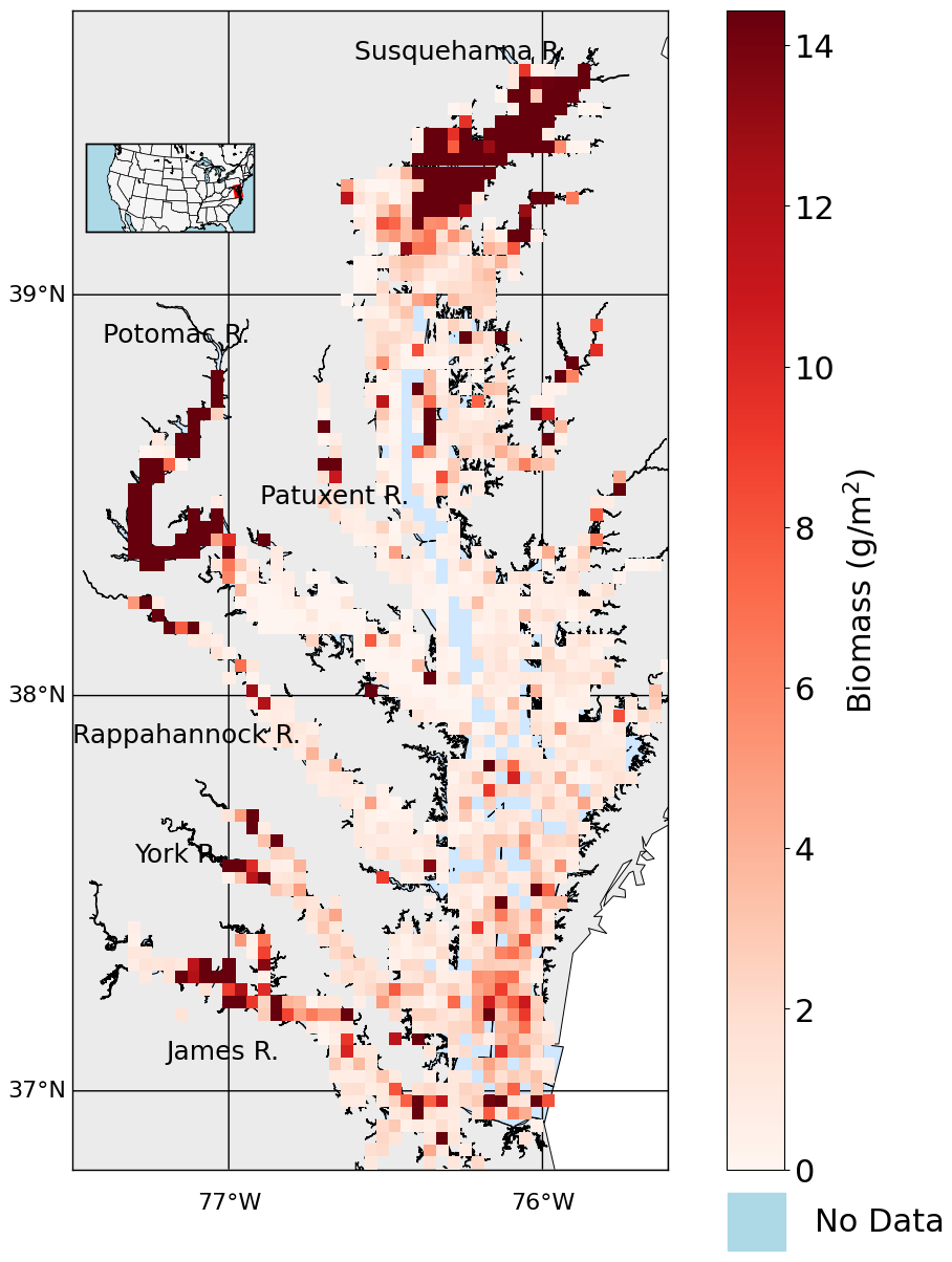
Figure 2 Average summer biomass density from 1995 to 2022 from the Chesapeake Bay Benthic Monitoring Program. Biomass values are shown using a red color scale, white represents 0 g m⁻², light blue indicates open water grid cells with no data, and gray represents land areas with no data.

The distribution of the biomass into salinity zones for multiple taxonomic groups and species is shown in Fig. 3b–f. Bivalves dominate biomass in all salinity zones, except the polyhaline, where they are comparable to polychaetes. Bivalves comprise 88.0 % of the benthic biomass, and polychaetes comprise 7.3 %. At a taxonomic species level, the bivalve R. cuneata comprises 66.1 % of the biomass, followed by the bivalves C. fluminea (8.0 %) and L. balthica (7.5 %). Appendix D provides a more detailed spatial analysis of species distribution. The high-biomass zones in the Upper Bay, Potomac River Estuary, and James River Estuary are dominated by R. cuneata, mostly in the oligohaline zone (Figs. 3c and D1). C. fluminea also dominates in relatively higher quantities in the tidal fresh zone of the Potomac River Estuary and the tidal fresh zone of the Upper Bay (Figs. 3d and D1). In general, R. cuneata has a higher biomass density in the tidal fresh than C. fluminea because R. cuneata is present in all tidal fresh zones. L. balthica is distributed in multiple salinity zones; it is highest in the lower mesohaline and is the dominant species in the lower mesohaline zone of the Upper Bay and Patuxent River Estuary (Figs. 3e and D1). The biomass density of L. balthica in the lower mesohaline (<2 g m⁻²) is significantly lower than that of C. fluminea and R. cuneata in the tidal fresh and oligohaline zones. Polychaetes are the species that dominate over the largest geographic area, throughout the polyhaline and part of the higher mesohaline (Figs. 2, 3f, and D1). However, their biomass density is low relative to bivalves (< 2 g m⁻²). Bivalves are sparse throughout the higher mesohaline and polyhaline zones.

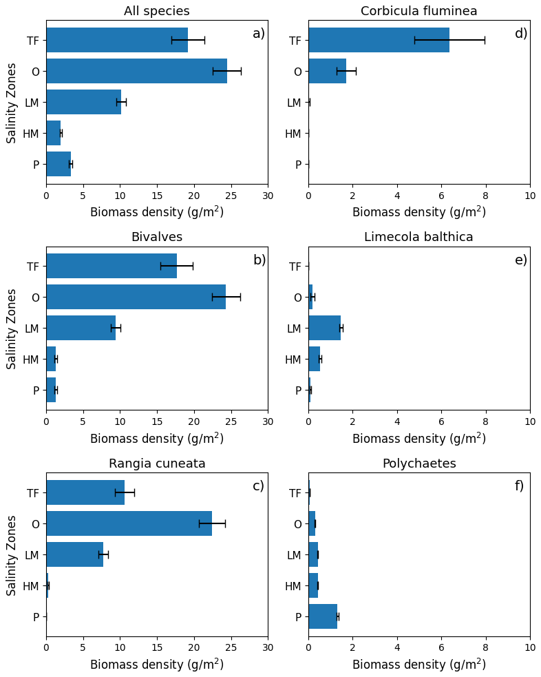
Figure 3 Average summer benthic biomass density of multiple classes and species in each salinity zone from 1995 to 2022. The salinity zones are determined by the BMP based on the long-term average of salinity in each geographic zone: TF – Tidal Freshwater (0–0.5 ppt), O – Oligohaline (0.5–5 ppt), LM – Low Mesohaline (5–12 ppt), HM – High Mesohaline (12–18 ppt), and P – Polyhaline (≥18 ppt). Averages and standard errors (bars) are computed using the full data set, not the gridded values. Note the difference in horizontal scale between the left and right columns.

3.2 Carbon flux estimates

Average benthic macrofaunal carbon and alkalinity fluxes vary across the 10 regions of the Bay (Fig. 4). Among the different fluxes, which are all presented on a molar basis in Fig. 4, F_TA has the largest magnitude, followed, in decreasing order, by $F_{{\mathrm{CO}}_{\mathrm{2}}}$, respiration ($R/M_{\mathrm{C}}$), calcification ($C/M_{{\mathrm{CaCO}}_{\mathrm{3}}}$), and F_DIC. We first discuss calcification, respiration, F_TA, and F_DIC. Calcification is 1.55 times respiration (best estimate), as a result of the molar ratio of these processes (Sect. 2.3.3). F_TA is always negative, as expected because calcification is an alkalinity sink, and twice the magnitude of calcification (Eq. 12). The best estimate of F_DIC was mostly positive, though it could be positive or negative because calcification is a DIC sink and respiration is a DIC source (Eq. 13). The best estimate of F_DIC ends up being positive because respiration exceeds calcification. Using the best estimate of the molar respiration:calcification ratio (1.55) and Equations 12 and 13, it can be shown that $-F_{\mathrm{TA}}/F_{\mathrm{DIC}}=\mathrm{3.6}$, consistent with the results in Fig. 4. Estimated uncertainties (Appendix B) were approximately 45 % for calcification, 40 % for respiration, 135 % for F_DIC, and 45 % for F_TA. The uncertainty for F_DIC being greater than 100 % admits the possibility of negative DIC fluxes.

$F_{{\mathrm{CO}}_{\mathrm{2}}}$ is always positive because benthic macrofauna remove TA from and add DIC to the water column. The magnitude of $F_{{\mathrm{CO}}_{\mathrm{2}}}$ can be understood by first noting that it is proportional to F_TA and F_DIC, with proportionality constants of $\left[{\mathrm{CO}}_{\mathrm{2}}\right]{\mathit{\zeta }}_{\mathrm{TA}}/\left[\mathrm{TA}\right]$ and $\left[{\mathrm{CO}}_{\mathrm{2}}\right]{\mathit{\zeta }}_{\mathrm{DIC}}/\left[\mathrm{DIC}\right]$, respectively (Eq. 17; note that F_TA<0 and ζ_TA<0, leading to $F_{{\mathrm{CO}}_{\mathrm{2}}}\mathit{>}\mathrm{0}$). In the open ocean, using mean conditions of pCO₂=400 µatm, [TA] = 2300 µmol kg⁻¹, temperature = 15 °C, and salinity = 35, we can use carbonate system equilibria to estimate [CO₂]∼ 15 µmol kg⁻¹, [DIC]∼ 2100 µmol kg⁻¹, and $-{\mathit{\zeta }}_{\mathrm{TA}}\sim$ ζ_DIC=11, which leads to $F_{{\mathrm{CO}}_{\mathrm{2}}}$ about 7 %–8 % of −F_TA and F_DIC. Here, we are seeing $F_{{\mathrm{CO}}_{\mathrm{2}}}$ comparable in magnitude to F_TA and F_DIC because Bay waters tend to have higher [CO₂] and ζ_DIC and lower [TA] and [DIC] than what is observed in open-ocean waters, as we show in Appendix E and Fig. E1. We observe much larger $F_{{\mathrm{CO}}_{\mathrm{2}}}$ in tidal fresh (6–18 mol m⁻² yr⁻¹) compared to oligohaline (3–7 mol m⁻² yr⁻¹) waters (Fig. 4), despite comparable values of F_DIC and F_TA. These differences in $F_{{\mathrm{CO}}_{\mathrm{2}}}$ between tidal zones are primarily driven by [CO₂], which is much higher in the tidal fresh due to a lower TA:DIC ratio (Fig. E1l). The magnitudes of the buffer factors are also greater in lower salinity waters (Figs. E1g and E1h), decreasing slightly in the polyhaline. Polyhaline values (13–16) are comparable to oceanic estimates of 9–15 (Egleston et al., 2010).

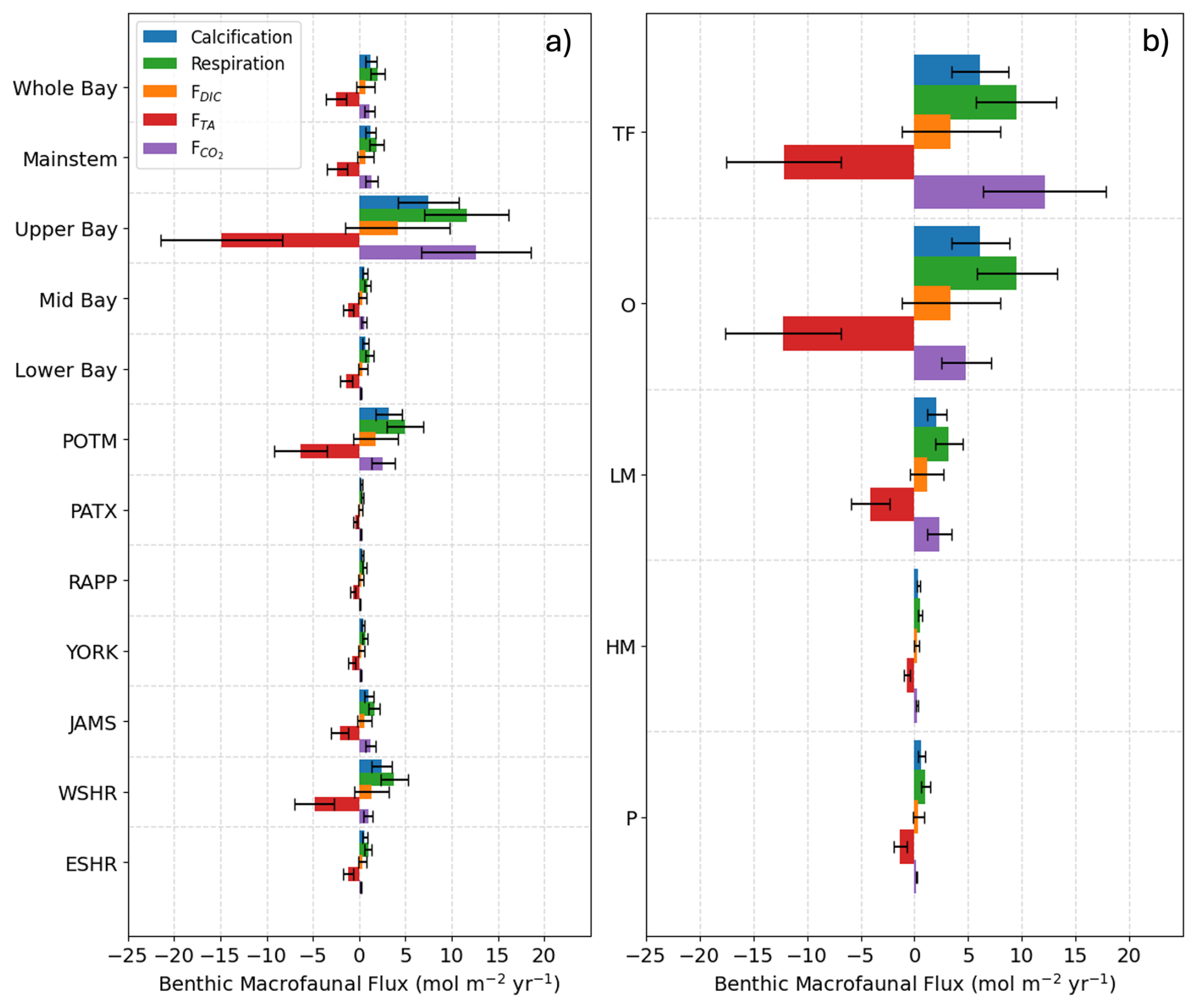
Figure 4 Average benthic macrofaunal fluxes by (a) Bay region and (b) salinity zone. Tributary and sub-estuarine acronyms: ESHR – Eastern Shore tributaries; WSHR – Western Shore tributaries; POTM – Potomac River; PATX – Patuxent River; RAPP – Rappahannock River; YORK – York River system (including Mattaponi and Pamunkey Rivers); JAMS – James River. Salinity zone abbreviations: TF – Tidal Freshwater (0–0.5 ppt), O – Oligohaline (0.5–5 ppt), LM – Low Mesohaline (5–12 ppt), HM – High Mesohaline (12–18 ppt), P – Polyhaline (≥18 ppt). Error bars represent uncertainty ranges (Appendix B).

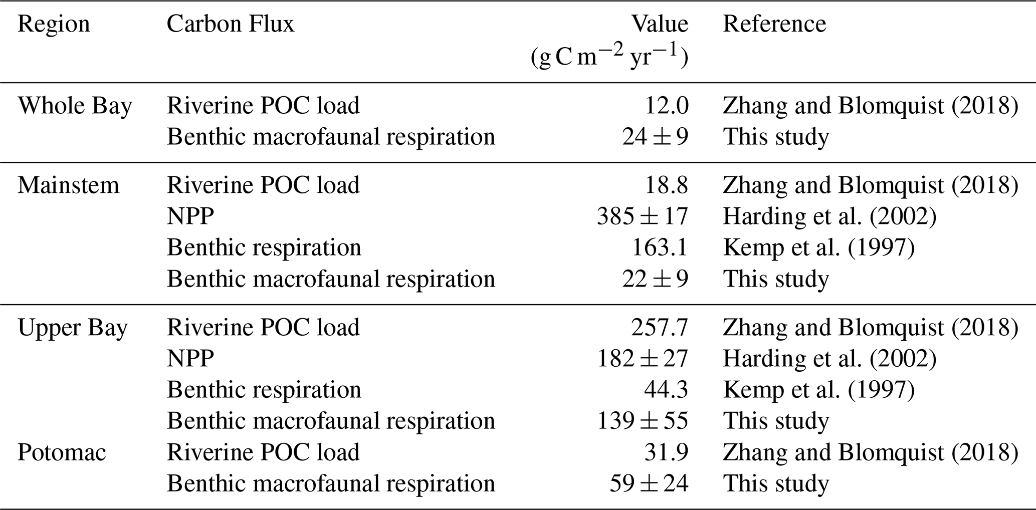
In multiple segments of the Bay, benthic macrofaunal respiration rates (R) are comparable to the total available organic carbon supply, defined here as the sum of net primary production (NPP) and riverine POC loads (Table 2). In the Upper Bay, benthic macrofaunal respiration rates are within the range of NPP alone. When combined with POC loads, our estimates suggest that benthic macrofauna respire approximately f=18 %–45 % of the total available organic carbon, where:

$$\begin{array}{}\text{(18)}& {\displaystyle }f={\displaystyle \frac{R}{\mathrm{NPP}+\mathrm{POC}}}\text{(19)}& {\displaystyle \frac{\mathrm{\Delta }f}{f}}=\sqrt{{\left({\displaystyle \frac{\mathrm{\Delta }R}{R}}\right)}^{\mathrm{2}}+{\left({\displaystyle \frac{\mathrm{\Delta }\mathrm{NPP}}{\mathrm{NPP}}}\right)}^{\mathrm{2}}}\end{array}$$

Here, ΔR and ΔNPP are the standard errors of R and NPP, respectively. This formulation is consistent with the uncertainty propagation approach described in Appendix B.

In the Potomac River Estuary, respiration rates exceed external organic carbon loads, although NPP estimates for this region were unavailable. By contrast, in the mainstem and across the Bay as a whole, benthic respiration rates are much smaller than NPP, accounting for only 3 %–8 % of the total inputs of organic carbon to the mainstem. These percentages were calculated using the same approach as in Eqs. (18)–(19), but substituting mainstem benthic macrofaunal respiration, NPP, and POC inputs.

Table 2 Riverine POC load, NPP, and benthic respiration compiled from the listed studies compared with benthic macrofaunal respiration from our study. POC load estimates from Zhang and Blomquist (2018) were based on USGS river monitoring data combined with flow-weighted sediment and organic carbon concentrations. For POC loads we specifically used values from Table S5 of Zhang and Blomquist (2018), which reports long-term average true-condition annual loads. Susquehanna loads were distributed across the mainstem and Upper Bay, Potomac River loads were distributed across the Potomac, and total watershed load was distributed across the whole Bay. These loads were divided by the surface area of the corresponding segment area (Chesapeake Bay Program, 2004). NPP values from Harding et al. (2002) were derived from depth-integrated in situ ¹⁴C-uptake incubations across multiple cruises, scaled using statistical models. Benthic respiration values from Kemp et al. (1997) were estimated by combining seasonal in situ measurements of sediment oxygen consumption with sulfate reduction rates, together accounting for microbial and macrofaunal respiration.

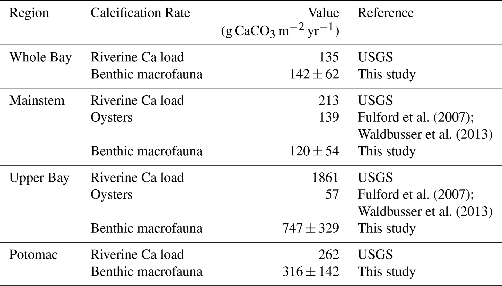
Benthic macrofauna also contribute substantially to the calcium budget of the Bay. We estimate that calcification by benthic macrofauna monitored in the BMP is slightly lower than historical (pre-decline) estimates of the Eastern oyster (Crassostrea virginica) calcification in the mainstem Bay but exceeds post-decline estimates by about 7 to 19 times in the Upper Bay (Table 3). This range was calculated by taking the upper and lower bounds of our measured calcification rates (mean ± uncertainty) and dividing each by the post-decline oyster calcification rate. Evaluating the role of bivalve calcification in utilizing calcium further underscores its biogeochemical significance. Relative to annual riverine calcium fluxes, benthic macrofauna would use ∼ 22 %–58 % of the available calcium in the Upper Bay and nearly all in the Potomac River. These percentages were likewise calculated by taking the lower and upper bounds of our measured calcification rates (mean ± uncertainty) and dividing each by the corresponding maximum potential riverine calcium input, which was treated as fixed.

Table 3 Historic oyster calcification rates and estimated maximum potential calcification based on riverine calcium input, compared with calcification rates from this study. Riverine calcium load from the Susquehanna River was distributed across the Upper Bay and across the mainstem, calcium load from the Potomac River was distributed within the Potomac segment, and the sum of all riverine calcium inputs was distributed across the Whole Bay.

The role of benthic macrofaunal metabolic processes in the carbon budget is particularly pronounced when the effects of calcification and respiration are combined to estimate CO₂ production. This CO₂ flux exceeds the amount of outgassing estimated in the Upper Bay and the mainstem overall (Table 4).

Table 4 Air–sea gas exchange from the listed studies compared with total benthic macrofaunal CO₂ flux calculated in our study.

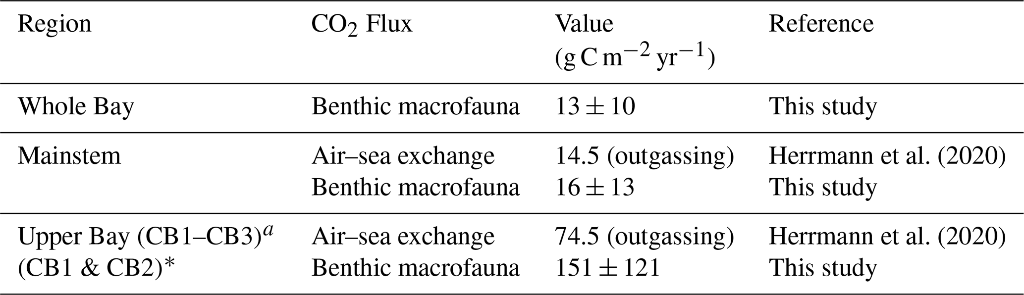
^* CB1–CB3 refer to Chesapeake Bay Program segmentation units (Chesapeake Bay Program, 2004): CB1 = tidal fresh, CB2 = oligohaline; CB3 = mesohaline.

3.3 Correlation of environmental variables with biomass

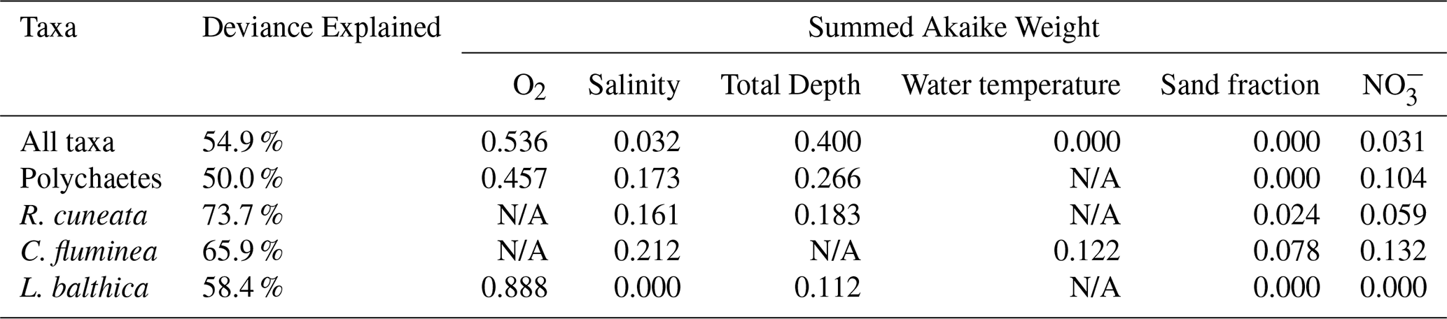
The GAMs analysis, based on gridded, time-averaged biomass data, revealed key drivers of benthic biomass both at the community level (all taxa combined) and for specific taxonomic groups and species. The results for total benthic biomass (all taxa), polychaetes, and the bivalve species R. cuneata, C. fluminea, and L. balthica are shown in Table 5. The bivalve group was excluded from the table because its results were nearly identical to total benthic biomass results. For total benthic biomass, the predictor variables (O₂, salinity, total depth, water temperature, sand fraction, and NO${}_{\mathrm{3}}^{-}$) explain 54.9 % of the deviance in biomass. For individual taxa, the predictive capability of GAMs increases, with 73.7 % of R. cuneata biomass deviance explained by the predictor variables. For total benthic biomass, dissolved oxygen emerged as the strongest predictor (with the highest summed Akaike weight), followed by total depth, salinity, and NO3⁻. Although water temperature and sand fraction were included in the model, they had relatively little influence. For individual taxa, dissolved oxygen became less influential, especially for R. cuneata and C. fluminea. Salinity generally increased in influence as a predictor variable for species-specific models, most notably for C. fluminea. NO${}_{\mathrm{3}}^{-}$ also generally increased in influence as a predictor variable for species-specific models, with very high influence as a predictor of C. fluminea biomass.

Table 5 The best-fitting generalized additive model (GAM) for each taxa assemblage, determined by minimizing Akaike's Information Criterion (AIC). N=846 (number of grid boxes with data) for all models. Summed Akaike weights indicate the relative importance of each predictor variable across all models considered, with higher values suggesting stronger support for a variable's inclusion in the best-fitting models. “N/A” indicates that the variable was not included in the best model. Some variables may have high summed Akaike weights even if they are not in the best-fitting model. For example, in the R. cuneata model, O₂ has a summed Akaike weight of 0.571, while water temperature has 0.032. In the C. fluminea model, O₂ has 0.384, and total depth has 0.24.

The relative effects of O₂, salinity, NO${}_{\mathrm{3}}^{-}$ and total depth on benthic biomass varied considerably, as shown in the partial plots of Fig. 5. Macrofauna biomass reaches its lowest values at low dissolved oxygen, the only section of all the partial plots that reach 0 g m⁻². Biomass is generally higher at shallower depths, although the effect is small. Biomass is highest at both low and high salinities and high surface NO${}_{\mathrm{3}}^{-}$. In summary, biomass is highest at moderate dissolved oxygen, shallow depths, low or high salinities, and high NO${}_{\mathrm{3}}^{-}$.

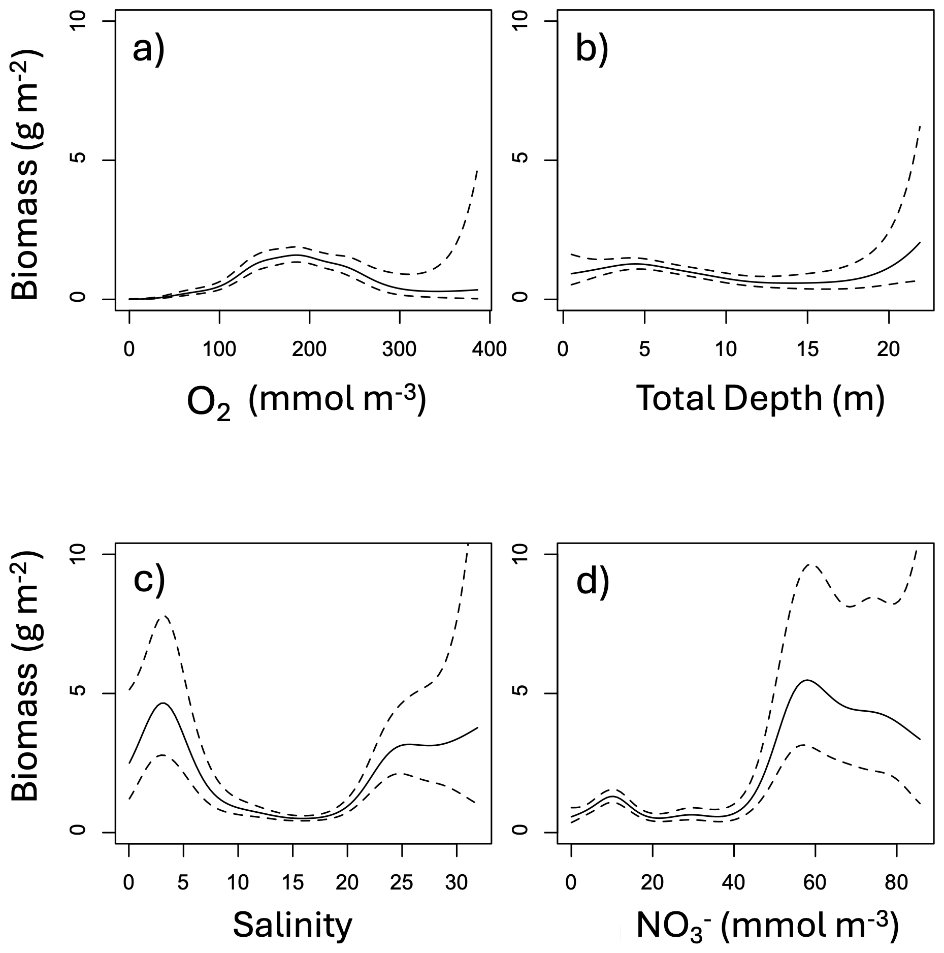
Figure 5 Partial plots of the effect of significant predictor variables on total biomass: (a) bottom dissolved oxygen, (b) total depth, (c) bottom salinity, and (d) surface nitrate. Water temperature and sand fraction were included in the model but omitted from display as they did not significantly improve the model fit. The solid black line shows the response and the dashed lines show the 95 % confidence interval. The natural log transformation was removed from biomass to enhance viewing of the partial plots. The x-axis was cut off at the upper quartile plus three interquartile ranges in order to remove extreme outliers from the plots.

The model fit evaluation, presented in Appendix F and Fig. F1, reveals some systemic biases. The residuals (observed values minus model-fitted values) are slightly skewed to the left (Fig. F1b), meaning the model is more likely to overestimate biomass. The response vs. fitted value scatter plot shows a nearly linear relationship (Fig. F1a). The map of residuals (Fig. F1c) shows that there is also an underestimation in the model fit at the high biomass zones, especially in the Upper Bay.

4 Discussion

4.1 Benthic macrofaunal contributions to the Chesapeake Bay carbon budget

The higher benthic biomass in less saline waters of the Chesapeake Bay suggests a significant role for respiration in the carbon budget in this region. The proportion of the total input of particulate organic carbon that is respired by benthic macrofauna estimated in our study in the Upper Bay (18 %–45 %) is similar to the 14 % to 40 % range estimated for bivalve filter feeders in tidal fresh and oligohaline waters by Cerco and Noel (2010). In the Upper Bay, where the benthic macrofauna respiration is comparable to NPP, if all the NPP were respired solely by benthic macrofauna, net ecosystem production would be zero. However, given the consideration of additional respiration by other organisms (e.g., microbes and pelagic zooplankton) the allochthonous POC from the Susquehanna River must be a critical source of organic carbon driving net heterotrophy in this region. These findings reinforce the earlier conclusion that high biomass zones in the Upper Bay are sustained by allochthonous organic inputs. The Potomac River Estuary, however, presents a less conclusive case, partly due to the lack of available NPP estimates. In this estuary, where benthic macrofaunal respiration exceeds the estimated POC flux, additional carbon sources, such as autochthonous NPP or tidal wetland outwelling, may be contributing to carbon metabolism. Notably, Herrmann et al. (2015) estimated that the amount of organic carbon exported through wetland outwelling is approximately equal to half of that exported by streamflow in Mid-Atlantic estuaries, highlighting its potential significance in supporting heterotrophic processes in the Potomac.

Benthic macrofaunal respiration plays a smaller role in the rest of the Bay, where autochthonous organic carbon dominates. For both the mainstem and the whole Bay, the estimated primary production far exceeds the average estimated benthic macrofaunal respiration, Kemp et al. (1997) estimated benthic respiration by combining sulfate reduction and sediment oxygen consumption rates, which together account for both microbial and macrofaunal respiration. Their results suggest that benthic respiration is a smaller fraction of NPP in the Mid and Lower Bay, compared to the Upper Bay. This may reflect the relatively modest role of macrofaunal respiration in these lower-biomass regions, despite higher autochthonous production and organic carbon delivery to the sediments. Our estimates of benthic macrofaunal respiration as a fraction of the total input of organic carbon to the mainstem (3 %–8 %) is slightly lower than estimates derived by Hopkinson and Smith (2004) and Rodil et al. (2022). Hopkinson and Smith (2004) estimated that approximately 24 % of total available organic carbon is respired by the benthos, while Rodil et al. (2022) found that benthic macrofauna account for roughly 40 % of total benthic respiration. Taken together, these studies suggest that around 10 % of the total input of organic carbon is expected to be respired by benthic macrofauna. Although the Bay-wide fraction is small, macrofaunal respiration may still dominate locally in specific hotspots.

Unlike the extensive research on estuarine benthic respiration, benthic macrofaunal calcification has received relatively little attention. Yet our findings suggest it may play a significant role in the Chesapeake Bay carbon budget. As shown in Table 3, bivalves sampled through the BMP program contribute substantially to calcification, surpassing calcification by present-day Eastern oyster populations but comparable to that of historic populations in the mainstem Bay. The importance of bivalve calcification is further emphasized when considering calcium dynamics. To place bivalve calcification in context, we assumed that all riverine calcium inputs were available for shell production. This is an upper-bound estimate because oceanic calcium greatly exceeds riverine fluxes (Beckwith et al., 2019). While not a full calcium budget, the comparison highlights how large the demand from calcification could be relative to the much smaller riverine supply. Alkalinity fluxes further highlight the biogeochemical significance of calcification. For the whole Bay, our estimated alkalinity consumption from benthic macrofaunal calcification of 2.52 ± 1.13 mol m⁻² yr⁻¹ (6.90 ± 3.10 mmol m⁻² d⁻¹) accounts for more than half of the Bay-wide alkalinity sink estimated by Waldbusser et al. (2013) at 12 mmol m⁻² d⁻¹. In the Potomac River Estuary, our estimated alkalinity sink due to benthic calcification (6.31 ± 2.84 mol m⁻² yr⁻¹ or 17.29 ± 7.78 mmol m⁻² d⁻¹) is comparable to the alkalinity sink of 22 ± 1 mmol m⁻² d⁻¹estimated by Najjar et al. (2020), who proposed that C. fluminea was primarily responsible. Our findings, highlighting contributions from both R. cuneata and C. fluminea, support their hypothesis and emphasize the substantial role of benthic calcification in modulating alkalinity in estuaries.

Benthic macrofauna may play a major role in CO₂ outgassing, as indicated by our estimated CO₂ fluxes from benthic macrofauna in the Upper Bay and upper tributaries, which exceed typical CO₂ fluxes at the air–sea interface. Our benthic macrofaunal CO₂ generation estimates for the Upper Bay (151 g C m⁻² yr⁻¹), where bivalve biomass is concentrated, exceed those reported by Chauvaud et al. (2003), who estimated 55 ± 51 g C m⁻² yr⁻¹ of CO₂ production from calcification and respiration by the bivalve P. amurensis in northern San Francisco Bay. Our results support their hypothesis that benthic calcifiers can serve as major CO₂ generators in estuaries. Not all of this CO₂ generated would be outgassed. However, the combination of a TA sink and DIC source from the bivalves leads to elevated pCO₂, enhancing the potential for increased CO₂ outgassing (Middelburg et al., 2020). Given the high heterotrophy in the Upper Bay and upper tributaries, as well as the balance between benthic macrofaunal respiration and the total input of organic carbon to the Potomac River Estuary, it is conceivable that benthic macrofauna are major contributors to CO₂ outgassing in these regions.

Although our empirical framework presented here captures the dominant patterns of benthic secondary production, it does not explicitly incorporate seasonal temperature variability. Because we applied summer temperatures associated with biomass, our production estimates likely represent the upper end of expected values. A simple sensitivity analysis comparing summer and winter conditions suggests that production, and by extension calcification and respiration, may be closer to 60 % of the values reported here under mean annual cycles. Importantly, this potential bias is encompassed within our uncertainty bounds and therefore does not affect our overall conclusions.

4.2 Environmental controls on benthic biomass distribution

Bivalve species distribution within the Bay is primarily driven by salinity tolerances. Both the GAMs analysis (Table 5) and the biomass densities associated with salinity zones (Fig. 3) showed that benthic biomass, dominated by bivalves, was much higher at lower salinities. The strong influence of salinity on benthic fauna distribution within estuaries has long been recognized (Cain, 1975; Hopkins et al., 1973). This relationship is illustrated in our study by the preference of the most abundant species, R. Cuneata, L. balthica, and C. fluminea, for less saline water. R. Cuneata is widely known to need less saline waters, optimally between 1 and 15 ppt, to survive (Hopkins et al., 1973). C. fluminea prefers freshwater environments (Phelps, 1994; Sousa et al., 2008). L. balthica has a range of tolerances but abundance declines below 5 ppt (Jansson et al., 2015). In our study, L. balthica is more concentrated between 5 and 13 ppt. While salinity determines which species dominate, other factors influence their relative abundances within salinity zones.

Within mesohaline zones, summer hypoxia appears to be driving extremely low benthic biomass. In our GAMs analysis, an association existed between low biomass and extremely low bottom dissolved oxygen values. Among the different salinity zones, low biomass is associated with low dissolved oxygen in the high mesohaline, where we had the lowest biomass densities. Long-term exposure to hypoxia (<2 mg L⁻¹ or 62.5 mmol m⁻³) is often fatal to benthic macrofauna (Diaz and Rosenberg, 1995; Seitz et al., 2006; Seitz et al., 2009) and many benthic communities (approximately 50 %) only recover on an annual timescale (Diaz and Rosenberg, 1995). In other words, regions that suffer frequent hypoxia often see lower levels of benthic biomass even when hypoxic conditions are not occurring. In the Chesapeake Bay, hypoxia is most likely to occur in the deeper, mesohaline regions (Frankel et al., 2022; Zheng and DiGiacomo, 2020), providing evidence that our suppressed values of benthic macrofauna at this salinity zone could be due to mass mortality from hypoxia. This pattern is particularly evident where biomass is extremely low through the Mid Bay and lower Potomac River Estuary, regions typically associated with summer hypoxia (Sturdivant et al., 2013).

Across the Bay, the relatively narrow range of summer bottom water temperatures likely explains why temperature has an insignificant effect on the spatial distribution of benthic biomass. In our GAMs analysis, summer bottom water temperature was not significantly correlated with benthic biomass. Water temperature has been considered an important driver of benthic biomass (Marsh and Tenore, 1990; Seitz et al., 2006; Seitz et al., 2009; Testa et al., 2020), with low temperature specifically creating mass mortality of R. cuneata during winter and spring (Tuszer-Kunc et al., 2020). Higher temperature, however, will drive early and larger seasonal hypoxia in the Chesapeake Bay (Hinson et al., 2022; Irby et al., 2018; Ni et al., 2019). So, temperature could still indirectly affect benthic biomass through its effect on dissolved oxygen. Therefore, while temperature many not directly drive spatial patterns of biomass, it could be more relevant to temporal changes in biomass.

Although NO${}_{\mathrm{3}}^{-}$ is a strong predictor of benthic biomass, the mechanisms are likely complex and not necessarily linked to autochthonous primary production. In upper estuarine zones, high NO${}_{\mathrm{3}}^{-}$ concentrations are often associated with elevated suspended solid loads, which limit light and may inhibit autotrophy (Brush et al., 2020). Yet these same areas show strong heterotrophy, suggesting that respiration exceeds local production. Prior studies have shown that POC in upper estuaries contains substantial terrigenous inputs (Canuel and Hardison, 2016), and respiration of this organic matter likely contributes to heterotrophy in these regions (Kemp et al., 1997; Testa et al., 2020). This pattern raises the possibility that NO${}_{\mathrm{3}}^{-}$ may serve as a proxy for allochthonous POC delivery. Supporting this, USGS data compiled by Zhang and Blomquist (2018) indicate that tributaries with high NO${}_{\mathrm{3}}^{-}$ also tend have high loads of POC. However, further study is needed to test this hypothesis, and the observed NO${}_{\mathrm{3}}^{-}$–POC correlation should not be interpreted as causal.

Our model explained roughly half of the deviance in biomass, indicating that environmental predictors captured key bottom-up controls. However, our model did not account for top-down factors such as predation, which may also play a significant role in shaping biomass distributions, particularly in an estuary with a densely populated watershed and substantial fishing pressure.

5 Conclusion

This study quantifies estuarine-scale benthic macrofaunal biomass and associated carbon fluxes, including secondary production, respiration, and calcification, across the Chesapeake Bay. The results demonstrate that benthic macrofauna play a substantial and spatially structured role in estuarine carbon cycling, particularly in upper estuarine zones where biomass is highest. In these regions, benthic macrofauna respiration is a significant fraction of total available organic carbon inputs, up to 45 %, while calcification accounts for a large portion of the observed alkalinity sink. These contributions vary across the salinity gradient, shaped by both environmental drivers and taxonomic composition.

Patterns observed in this study suggest that benthic biomass and its associated carbon fluxes are influenced by gradients in salinity, oxygen, and organic matter inputs. The dominance of bivalves in low-salinity zones has particularly strong biogeochemical implications due to the role of bivalves in secondary production and calcification. Notably, NO${}_{\mathrm{3}}^{-}$ emerged as a strong predictor of benthic biomass, not necessarily due to enhanced autotrophic production, but potentially reflecting allochthonous organic matter inputs that drive heterotrophic metabolism. The significant contributions of benthic communities to alkalinity consumption and DIC release highlight their potential to alter estuarine carbon chemistry in ways that depend on both biological composition and environmental conditions.

To build on these results, future work should examine how benthic biomass and associated carbon fluxes vary over time in response to both natural variability and anthropogenic change. Predicting future responses is especially challenging due to the high-frequency variability in estuarine systems, which can obscure long-term signals. Understanding how POC inputs, particularly allochthonous sources, change seasonally and interannually will be critical, as will clarifying the extent to which NO${}_{\mathrm{3}}^{-}$ serves as a proxy for those inputs. Long-term monitoring and modeling efforts that link changes in watershed nutrient loading, land use, and climate with benthic community dynamics will be essential for forecasting ecosystem responses and for developing more accurate, responsive biogeochemical models. These predictive relationships between benthic biomass and environmental conditions could also support management and restoration planning. By identifying areas where oxygen, salinity, or sediment improvements are most likely to enhance benthic productivity, the models provide a framework for prioritizing restoration efforts and assessing ecosystem responses to changing conditions.

Appendix A: Biomass Sampling Density

This appendix shows the spatial distribution of sampling effort for the BMP from 1995 to 2022. Figure A1 illustrates the number of samples collected in each grid cell, highlighting areas of higher and lower sampling density across the Chesapeake Bay and its tributaries.

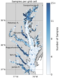
Figure A1 Number of benthic samples collected in each grid cell in the summer (15 July to 30 September) from 1995 to 2022 from the Chesapeake Bay Benthic Monitoring Program. The grids are approximately square, measuring 3.5 km by 3.5 km. Each grid cell contains a time-average of each measurement collected in the cell.

Appendix B: Carbon flux uncertainties

This appendix explains the methodology for propagating uncertainty in the benthic macrofaunal carbon flux estimates. It outlines the parameter ranges used, the calculations for uncertainty bounds, and the assumptions underlying these estimates. These details support the uncertainty ranges shown in figures and tables in the Results section. Uncertainty estimates were propagated through empirical equations using standard error propagation techniques (Taylor, 2022) assuming uncorrelated inputs and approximating relative errors when only a range of values was available.

Uncertainty for carbon-based biomass (B_c) is derived from the two different r_c values:

$$\begin{array}{}\text{(B1)}& {\displaystyle \frac{\mathrm{\Delta }{B}_{\mathrm{c}}}{B_{\mathrm{c}}}}={\displaystyle \frac{\mathrm{\Delta }{r}_{\mathrm{c}}}{r_{\mathrm{c}}}}\end{array}$$

where Δ r_c=0.03 g C g⁻¹, half the range of possible r_c values.

The uncertainty for the first approach for estimating secondary production (S₁) is derived from B_c and α:

$$\begin{array}{}\text{(B2)}& {\displaystyle \frac{\mathrm{\Delta }{S}_{\mathrm{1}}}{S}}=\sqrt{{\left({\displaystyle \frac{\mathrm{\Delta }\mathit{\alpha }}{\mathit{\alpha }}}\right)}^{\mathrm{2}}+{\left({\displaystyle \frac{\mathrm{\Delta }{B}_{\mathrm{c}}}{B_{\mathrm{c}}}}\right)}^{\mathrm{2}}}\end{array}$$

Δ α is half the range of possible α values and equals 1.695 yr⁻¹.

Uncertainty in secondary production (S) arises from the multiple equations used:

$$\begin{array}{}\text{(B3)}& \mathit{\epsilon }{\displaystyle \frac{\mathrm{\Delta }S}{S}}=\sqrt{w{\left({\displaystyle \frac{\mathrm{\Delta }{S}_{\mathrm{1}}}{S_{\mathrm{1}}}}\right)}^{\mathrm{2}}+\mathrm{2}w}\end{array}$$

where each model is equally weighted ($w=\mathrm{1}/\mathrm{3}$). Only Model 1 (Eq. 5) includes an explicit source of uncertainty, while Models 2 and 3 (Eqs. 7 and 8) do not. Therefore a small error term ε=0.001 was assumed for those two models.

Calcification (C) uncertainty is derived from r_s and S:

$$\begin{array}{}\text{(B4)}& {\displaystyle \frac{\mathrm{\Delta }C}{C}}=\sqrt{{\left({\displaystyle \frac{\mathrm{\Delta }{r}_{\mathrm{s}}}{r_{\mathrm{s}}}}\right)}^{\mathrm{2}}+{\left({\displaystyle \frac{\mathrm{\Delta }S}{S}}\right)}^{\mathrm{2}}}\end{array}$$

where r_s has one value for C. fluminea and one for P. amurensis. Δr_s=2.5 g CaCO₃ (g C⁻¹) and is half the range of possible r_s values.

The uncertainty in respiration (R) is derived solely from S:

$$\begin{array}{}\text{(B5)}& \mathrm{\Delta }R=\mathrm{2.33}\mathrm{\Delta }S\end{array}$$

The uncertainties in the fluxes of alkalinity and DIC (F_TA and F_DIC) are also derived from C and R:

$$\begin{array}{}\text{(B6)}& {\displaystyle }\mathrm{\Delta }{F}_{\mathrm{TA}}={\displaystyle \frac{-\mathrm{2}\mathrm{\Delta }C}{M_{{\mathrm{CaCO}}_{\mathrm{3}}}}}\text{(B7)}& {\displaystyle }\mathrm{\Delta }{F}_{\mathrm{DIC}}=\sqrt{{\left({\displaystyle \frac{\mathrm{\Delta }R}{M_{\mathrm{C}}}}\right)}^{\mathrm{2}}+{\left({\displaystyle \frac{\mathrm{\Delta }C}{M_{{\mathrm{CaCO}}_{\mathrm{3}}}}}\right)}^{\mathrm{2}}}\end{array}$$

where $M_{{\mathrm{CaCO}}_{\mathrm{3}}}$ and M_C are the molar masses of CaCO₃ and C, respectively.

Finally, we propagate the error in the flux of carbon dioxide ($F_{{\mathrm{CO}}_{\mathrm{2}}}$) from the errors in F_TA and F_DIC:

$$\begin{array}{}\text{(B8)}& \mathrm{\Delta }{F}_{{\mathrm{CO}}_{\mathrm{2}}}=\sqrt{{\left({\displaystyle \frac{\left[{\mathrm{CO}}_{\mathrm{2}}\right]{\mathit{\zeta }}_{\mathrm{TA}}\mathrm{\Delta }{F}_{\mathrm{TA}}}{\left[\mathrm{TA}\right]}}\right)}^{\mathrm{2}}+{\left({\displaystyle \frac{\left[{\mathrm{CO}}_{\mathrm{2}}\right]{\mathit{\zeta }}_{\mathrm{DIC}}\mathrm{\Delta }{F}_{\mathrm{DIC}}}{\left[\mathrm{DIC}\right]}}\right)}^{\mathrm{2}}}\end{array}$$

We do not consider errors in the buffer factors, [CO₂], [DIC], and [TA] in ROMS.

Appendix C: Secondary production model comparison

This appendix details the comparison of secondary production estimates from the three approaches described in Sect. 2.3.1. Seasonal and spatial variations are shown to illustrate the influence of temperature and other parameters on production estimates. These comparisons provide context for interpreting model differences presented in the main text.

The models have similar spatial patterns (Fig. C1), which are similar to the pattern of benthic biomass (Fig. 2). Secondary production is generally higher in Model 1 than in Models 2 and 3, which can be seen most clearly in the means, which are 17.92, 8.31, and 7.59 g C m⁻² yr⁻¹ in Models 1, 2, and 3, respectively.

Figures C2 and C3 compare secondary production between summer and winter scenarios. The summer scenario uses summer bottom water temperatures measured concurrently with biomass samples, while the winter scenario assumes a temperature of 1 °C. Figure C2 shows the results for Model 2, which has a mean secondary production of 8.31 g C m⁻² yr⁻¹ in summer and 1.89 g C m⁻² yr⁻¹ in winter. Figure C3 shows the results for Model 3, which has a mean secondary production of 7.59 g C m⁻² yr⁻¹ in summer and 1.44 g C m⁻² yr⁻¹ in winter. For both models, production in summer is about 5 times that of winter, as expected from the rough estimates in the Methods section. Assuming spring and fall are halfway between winter and summer, and weighting the seasons equally, the annually averaged secondary production rate would be about 60 % of the summer rate.

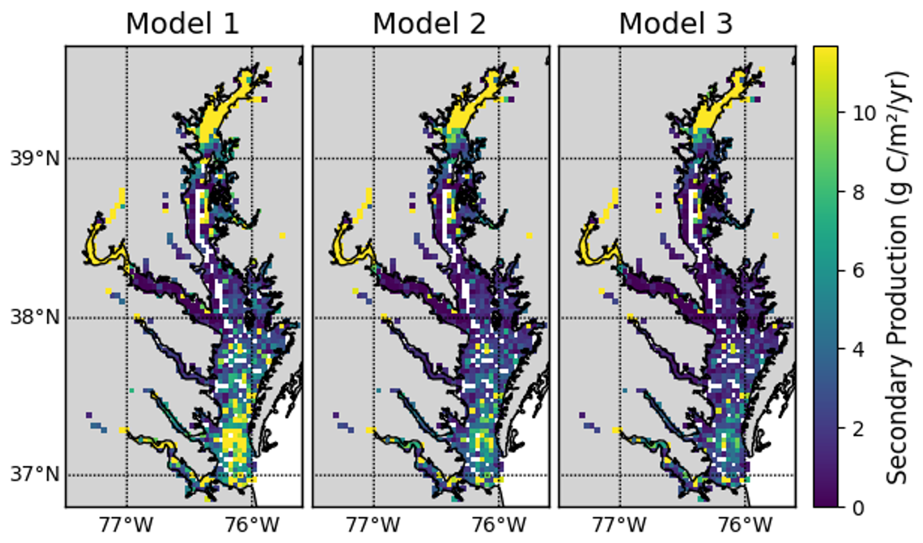
Figure C1 Long-term average secondary production across the Chesapeake Bay for each of the three secondary production models.

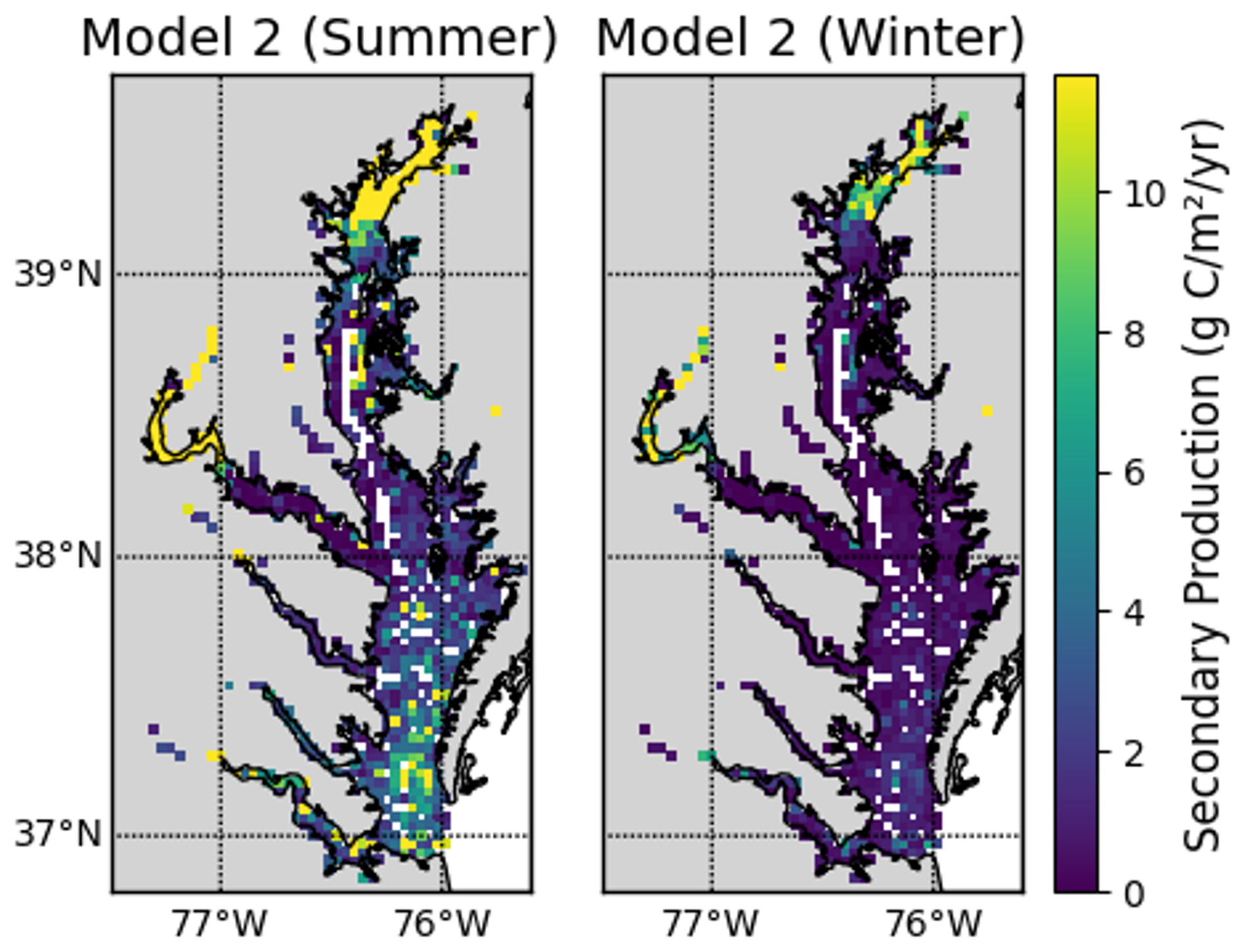
Figure C2 Seasonal sensitivity of Model 2 to bottom temperature inputs.

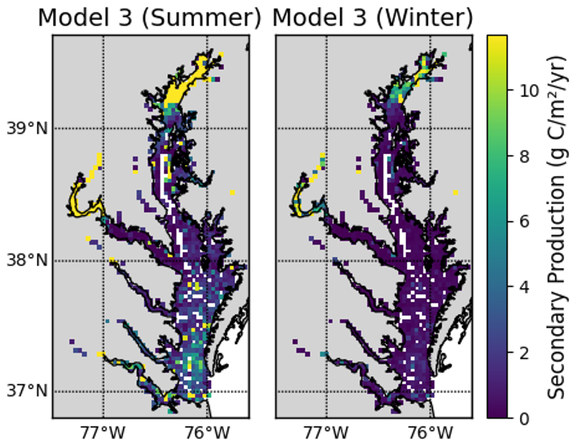
Figure C3 Seasonal sensitivity of Model 3 to bottom temperature inputs.

Appendix D: Species biomass distribution

This appendix expands on the biomass distribution results in Sect. 3.1 by showing detailed spatial patterns for individual species and taxonomic classes. Figure D1 complements the summary figures in the main text, highlighting species-specific habitat associations.

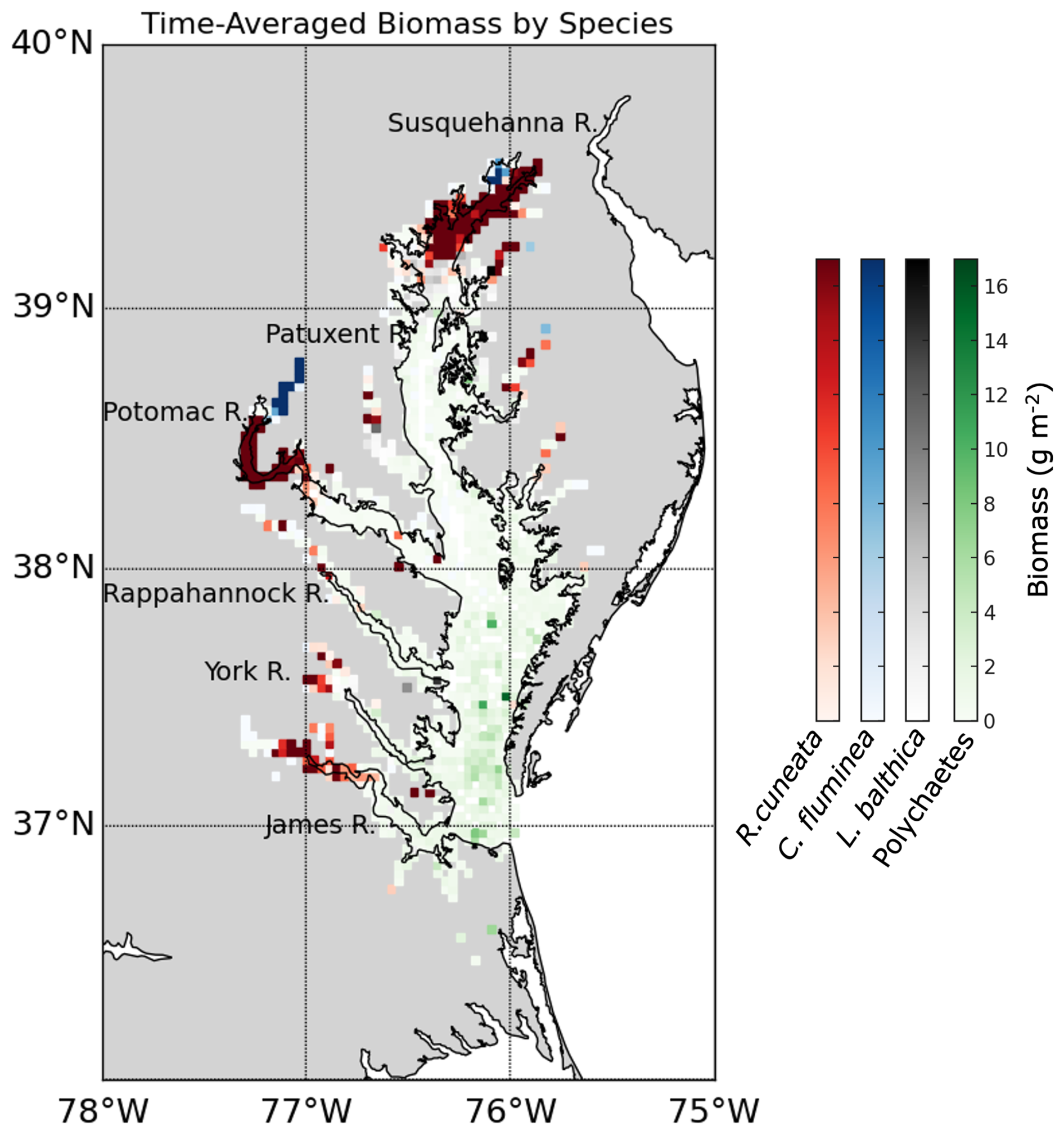
Figure D1 Average summer biomass density from 1995 to 2022 from the Maryland and Virginia Benthic Monitoring Program. Each color corresponds to a specific bivalve species (M. balthica, C. fluminea, or R. cuneata) or polychaetes. The color shown on the map is the species with the highest time-averaged biomass in that grid cell.

Appendix E: Carbon flux-related parameters

To illustrate estuarine variability in carbonate system drivers, we summarized a suite of flux and water column properties across tidal salinity zones of the Chesapeake Bay (Fig. E1). The patterns highlight strong gradients from tidal fresh through polyhaline regions. Notably [CO₂] is elevated in tidal fresh waters, underscoring the combined influence of salinity, TA, and the TA:DIC ratio on estuarine carbonate chemistry.

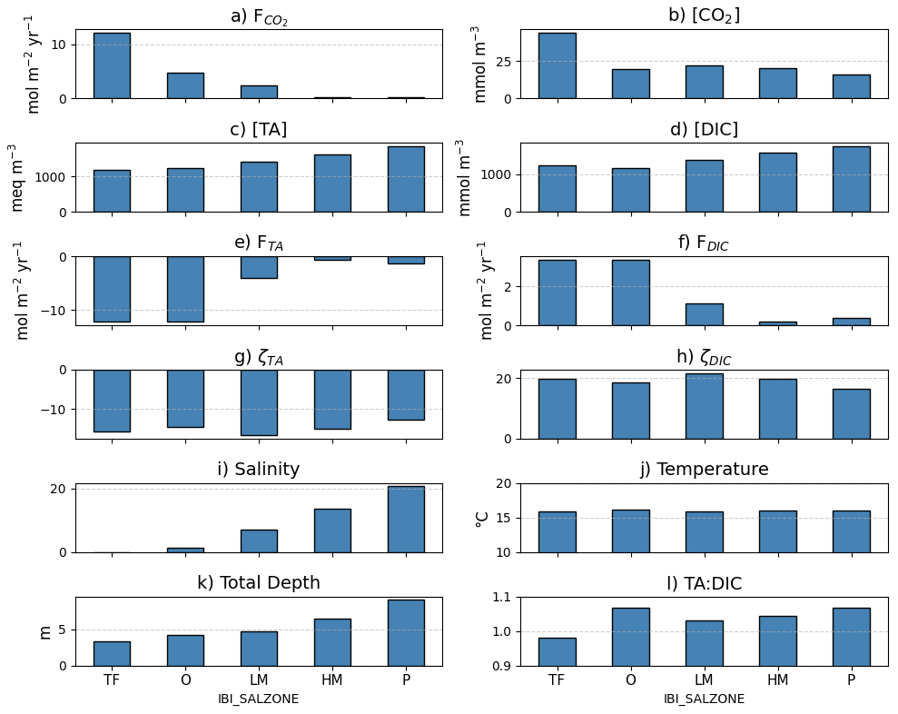
Figure E1 Carbon flux-related parameters averaged within salinity zones of Chesapeake Bay. [CO₂] was calculated using PyCO₂SYS; temperature, salinity, total depth, [TA] and [DIC] were obtained from ROMS model output. F_TA and F_DIC were calculated following Eqs. (12)–(13), ζ_TA and ζ_DIC from Eqs. (15)–(16), and $F_{{\mathrm{CO}}_{\mathrm{2}}}$ from Eq. (14).

Appendix F: GAMs evaluation

This appendix presents diagnostic plots and statistics for the generalized additive models described in Sect. 2.5. Residual maps, histograms, and fitted-vs-observed plots (Fig. F1) are included to evaluate model performance and identify patterns in prediction errors.

A good model would have points on a modeled vs. observed scatterplot fall close to a 1:1 line and have the departures from that line (residuals) be close to normally distributed. Although GAMs can handle non-normal distributions of the response variable (Guisan et al., 2002), we found the best model fit by applying a natural logarithmic transformation to the biomass. A small constant (0.0001 g m⁻²) was added to the biomass values before applying the natural logarithmic transformation to account for zeros in the data. The resulting biomass was normally distributed after applying the natural logarithm function, so the GAM was fitted with a Gaussian distribution with an identity link function.

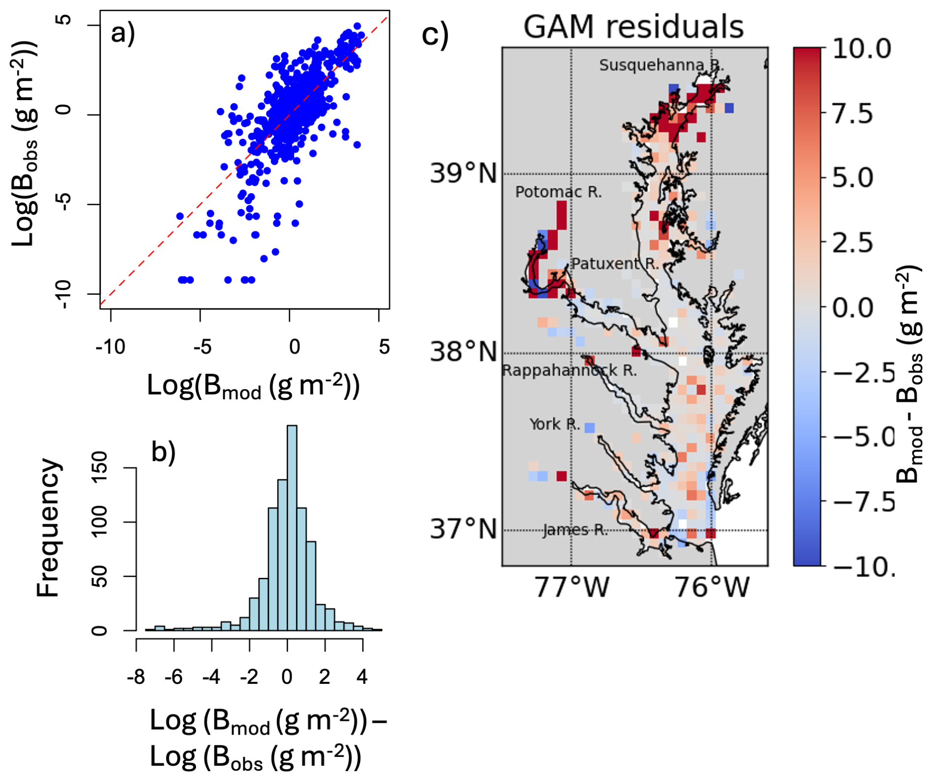
Figure F1 Evaluation of the total biomass GAM, which includes O₂, salinity, total depth, NO${}_{\mathrm{3}}^{-}$, sand fraction, and water temperature as predictor variables. “Log” refers to the natural logarithm. (a) Modeled vs. observed values. (b) Histogram of biomass residuals (modeled minus observed values, B_mod–B_obs). (c) Spatial distribution of the residuals.