Future diversity and lifespan of metazoans under global warming and oxygen depletion

The diversification of metazoans began approximately 700–500 million years ago, evolving from cnidarian-like ancestors into complex groups such as arthropods and vertebrates under dynamic environmental conditions. Throughout Earth's history, abrupt climate fluctuations – driven by large-scale volcanism and meteorite impacts – have repeatedly reshaped global biodiversity. Understanding these historical patterns provides critical insights into the long-term future of life under ongoing and future climate change. Here, I model the future ecosystem diversity of terrestrial metazoans – including insects and tetrapods – and marine metazoans by integrating multiple environmental drivers: solar-luminosity–induced warming, alternating icehouse–greenhouse cycles, progressive declines in atmospheric CO₂ and O₂, abrupt climate fluctuations, and anthropogenic impacts. The results indicate that family-level diversity of terrestrial insects, tetrapods, and marine metazoans – including subterranean and deep-water taxa – will begin to decline approximately 0.5 billion years from now, and ultimately vanish at around 0.9, 0.9, and 1.0 billion years, respectively. These projections hold across models both with and without evolutionary adaptation to extremely low CO₂ and O₂ conditions. The difference in extinction timing between land and ocean reflects lower maximum temperatures in marine environments. The primary driver of gradual biodiversity loss is the long-term reduction of atmospheric CO₂ and O₂ due to the steady increase in solar luminosity. However, extinction is completed by episodic warming events – primarily volcanic in origin – that exceed the thermal tolerance limits of metazoans when superimposed on gradual solar-driven warming. These findings offer a unified quantitative framework for understanding the far-future trajectory and ultimate limits of metazoan biodiversity on Earth.

1 Introduction

Metazoans first appeared and diversified around 700–500 million years ago, evolving from simple cnidarian-like organisms into more complex groups such as arthropods and vertebrates during intervals of rising oxygen and shifts from icehouse to greenhouse climates (Erwin, 2015; Kaiho et al., 2024). After transitioning onto land approximately 400 million years ago, metazoans eventually gave rise to humans (genus Homo) roughly 3 million years ago. Despite this long evolutionary history, the future trajectory of metazoan diversity remains poorly understood.

Estimates published after 2010 for the eventual collapse of Earth's biosphere vary widely. Projections based solely on long-term solar-driven warming range from 1.0 to 5.0 Gyr (O'Malley-James et al., 2013; Rushby, 2013; Leconte et al., 2013; Wolf and Toon, 2015). In contrast, CO₂-depletion models predict substantially earlier biosphere loss at 0.84–1.08 Gyr (Rushby, 2015; Ozaki and Reinhard, 2021). Mello and Friaça (2019) argue that thermal limits may delay biosphere collapse to ∼1.5 Gyr, whereas atmospheric O₂ is projected to fall to 1 % present atmospheric levels (PAL) within 1.08 ± 0.14 Gyr, potentially driving an earlier extinction of metazoans (Ozaki and Reinhard, 2021). Overall, current geosphere–biosphere models suggest a remaining biosphere lifespan of at least ∼0.8 Gyr, with ∼1.2 Gyr as a plausible median estimate (Jebari and Sandberg, 2022).

A gradual increase in solar luminosity is the primary driver of Earth's far-future climate (Franck et al., 2006; Abe et al., 2011; O'Malley-James et al., 2013; Mello and Friaça, 2019; Ozaki and Reinhard, 2021). Over the next 1.1 Gyr, global mean temperature is projected to rise from 14 to ∼40 °C (Mello and Friaça, 2019), while atmospheric and oceanic O₂ may decline to ∼1 % PAL (Ozaki and Reinhard, 2021). By ∼1.6 Gyr from now, temperatures may exceed 100 °C, rendering Earth uninhabitable for nearly all forms of life.

This warming accelerates continental weathering, which removes atmospheric CO₂ over timescales of hundreds of thousands of years, triggering cascading biological crises. Declining CO₂ will differentially affect C₃ and C₄ plants because of their distinct photosynthetic pathways: C₄ plants tolerate hotter, drier, low-CO₂ conditions better than C₃ plants. Thus, C₃ plants (including most trees) are expected to decline first, followed by C₄ plants, ultimately leading to collapse of metazoan ecosystems (Reinfelder et al., 2000, 2004; Mello and Friaça, 2019; Ozaki and Reinhard, 2021).

Superimposed on the long-term warming trend are ∼0.30–0.35 Gyr cyclic climate rhythms (Scotese et al., 2021; Torsvik et al., 2024; Vérard, 2024), driven primarily by plate-tectonic and mantle processes associated with supercontinent cycles (Heron, 2018). These influence long-term climate through changes in ocean circulation and atmospheric composition and may persist as long as mantle convection and oceans remain active – though future CO₂ depletion may dampen or terminate this cyclicity.

In addition, Earth's climate has repeatedly experienced abrupt perturbations. Large-scale volcanism and asteroid impacts have induced rapid global cooling followed by long-term warming (Kaiho, 2025), triggering mass extinctions throughout the past 500 Myr (Erwin et al., 1987; Sepkoski, 1996; Bambach, 2006; Kaiho, 2022a). Because these events unfold over tens to tens of thousands of years – shorter than continental-weathering timescales – they temporarily destabilize climate and can profoundly reshape biodiversity.

Despite their importance, neither cyclic nor abrupt events are incorporated into most long-term future-Earth models, leaving major uncertainties in forecasting Earth's biodiversity trajectory. Here, we integrate both types of events as drivers that impose “step changes” on biodiversity to evaluate how long animal life may persist on Earth.

This study further investigates extinction dynamics across superterranean, subterranean, surface-water, and deep-sea habitats. By integrating future projections of temperature, CO₂, and atmospheric oxygen with established physiological limits on metazoan thermal tolerance, oxygen requirements, and CO₂-driven effects on plants and climate, the model employs six major drivers – anthropogenic crises, long-term warming, cyclic climate rhythms, abrupt events, plant decline, and oxygen depletion – to forecast extinction trajectories for insects, terrestrial tetrapods, and marine metazoans over the next 1.5 billion years. These projections are grounded in documented diversity patterns throughout the Phanerozoic.

2 Methods

2.1 Method summary

To project the future lifespan of metazoans on Earth, I developed a multi-step model that integrates relationships derived from past climate behavior and biodiversity dynamics (Fig. 1). A key assumption is that the amplitude of long-term icehouse–greenhouse climate cycles – occurring at ∼0.35–0.30 Gyr intervals (Scotese et al., 2021; Torsvik et al., 2024; Vérard, 2024) – will gradually diminish as atmospheric CO₂ declines through enhanced continental weathering; for modeling purposes, these cycles are treated as having 0.30 Gyr intervals. In contrast, major abrupt climatic perturbations capable of triggering mass extinctions are assumed to continue recurring at ∼0.094 Gyr intervals, based on the mean recurrence time calculated from age data in Kaiho (2025). Importantly, the specific values chosen for these intervals do not influence the 0.1 Gyr–resolution results presented in the abstract.

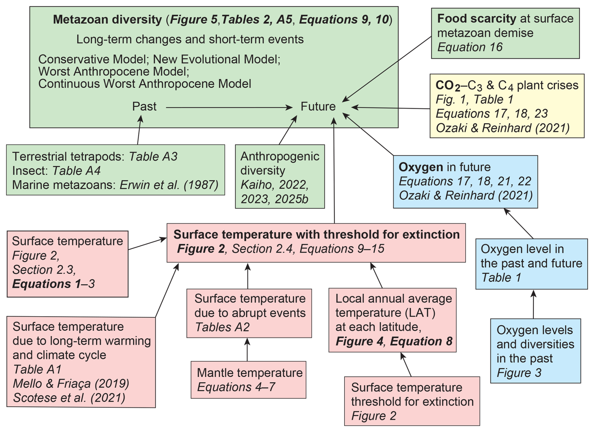
Figure 1 Flowchart illustrating the methodological framework used to estimate past and future metazoan diversity and thereby determine the lifespan of metazoans on Earth. The diagram summarizes the sequential steps leading to the projections shown in Fig. 5. Color coding highlights key controlling factors: red indicates temperature, blue represents atmospheric oxygen levels, yellow corresponds to atmospheric CO₂ concentrations, and green denotes metazoan diversity.

Abrupt events (Eq. 9) are treated independently from long-term climate change (Eq. 10), because their short duration means they are not significantly affected by the gradual evolution of climate. Accordingly, the equations in Sect. 2.5 are designed to calculate the number of families after an event (D_nR) based on the number of families before the event (D_(n−1)A). On the other hand, by combining temperature variations caused by long-term cyclic climate changes – driven by increasing solar radiation and declining mantle potential temperature – with those from abrupt events, and comparing the resulting habitat temperatures with the thermal tolerance limits of each animal group, the Survival Rate by Climates (SRC) in Sect. 2.5 can be derived.

The long-term increase in solar radiation leads to declines in both atmospheric oxygen and carbon dioxide. The progressive atmospheric CO₂ drawdown – accelerated by intensified continental weathering – will trigger recurrent plant crises, while a concurrent decline in atmospheric oxygen will ultimately lead to the extinction of metazoan life.

Since fluctuations in atmospheric oxygen and carbon dioxide have already been reported, those values are used to determine the proportional impact on the number of families for insects, terrestrial tetrapods, and marine animals. Based on these impacts and temperature changes, the number of families is calculated, and their trends are used to determine the timing of diversity shifts and eventual extinction.

The analysis proceeded through the following steps:

• A.

  Baseline reconstruction of historical diversity, climate, and oxygen levels (see Sect. 2.2).

• B.

  Projection of future temperature trends (see Sect. 2.3).

• C.

  Determination of metazoan thermal tolerance limits, where local extinction thresholds are scaled to global mean surface temperature based on latitudinal gradients (see Sect. 2.4).

• D.

  Development of an integrated future-diversity model, combining elements from steps A–C with long-term atmospheric CO₂ and O₂ projections, while accounting for food scarcity effects triggered by the collapse of surface-dwelling metazoans (see Sect. 2.5).

Future changes in metazoan diversity were evaluated under four modeled scenarios:

• D1.

  Conservative Model – assumes no full-scale nuclear conflict and conservative ecological responses without evolutionary adaptation to extreme CO₂ and O₂ deficiency.

• D2.

  New Evolutional Model – incorporates potential evolutionary adaptation to extremely low CO₂ and O₂ levels.

• D3.

  Worst Anthropocene Model – assumes a full-scale nuclear war followed by initial recovery (Kaiho, 2022b, 2023, 2026).

• D4.

  Continuous Worst Anthropocene Model – includes a full-scale nuclear war and ongoing anthropogenic pressures, resulting in prolonged biodiversity decline.

In addition to the standard simulations, supplementary test cases were conducted in which one causal parameter from steps A–D was held constant at its initial value throughout the entire 1.5 Gyr simulation period under the Conservative Model. These auxiliary simulations are not intended as realistic projections, but rather serve to elucidate the individual contributions of each parameter to the timing of metazoan extinction relative to the baseline models.

All datasets were generated using the equations and baseline data outlined in Sects. 2.2–2.5. All calculations were executed in Microsoft Excel, and the resulting data are presented in the accompanying tables.

2.2 Past diversity, climate, and oxygen baselines

To estimate future metazoan diversity, I compiled past records of global surface temperature and biodiversity. Earth's climate has displayed a recurring 0.35–0.30 Gyr cycle since ∼1.0 Gyr ago (Fig. 2), consisting of extended greenhouse phases lasting ∼0.2 Gyr followed by shorter ∼0.1 Gyr icehouse phases (Scotese et al., 2021; Torsvik et al., 2024; Vérard, 2024). To incorporate this cyclicity, I applied an 8 °C temperature anomaly between icehouse and greenhouse states (Scotese et al., 2021) to the Mello and Friaça model (Fig. 2, Tables S1 and S2 in the Supplement).

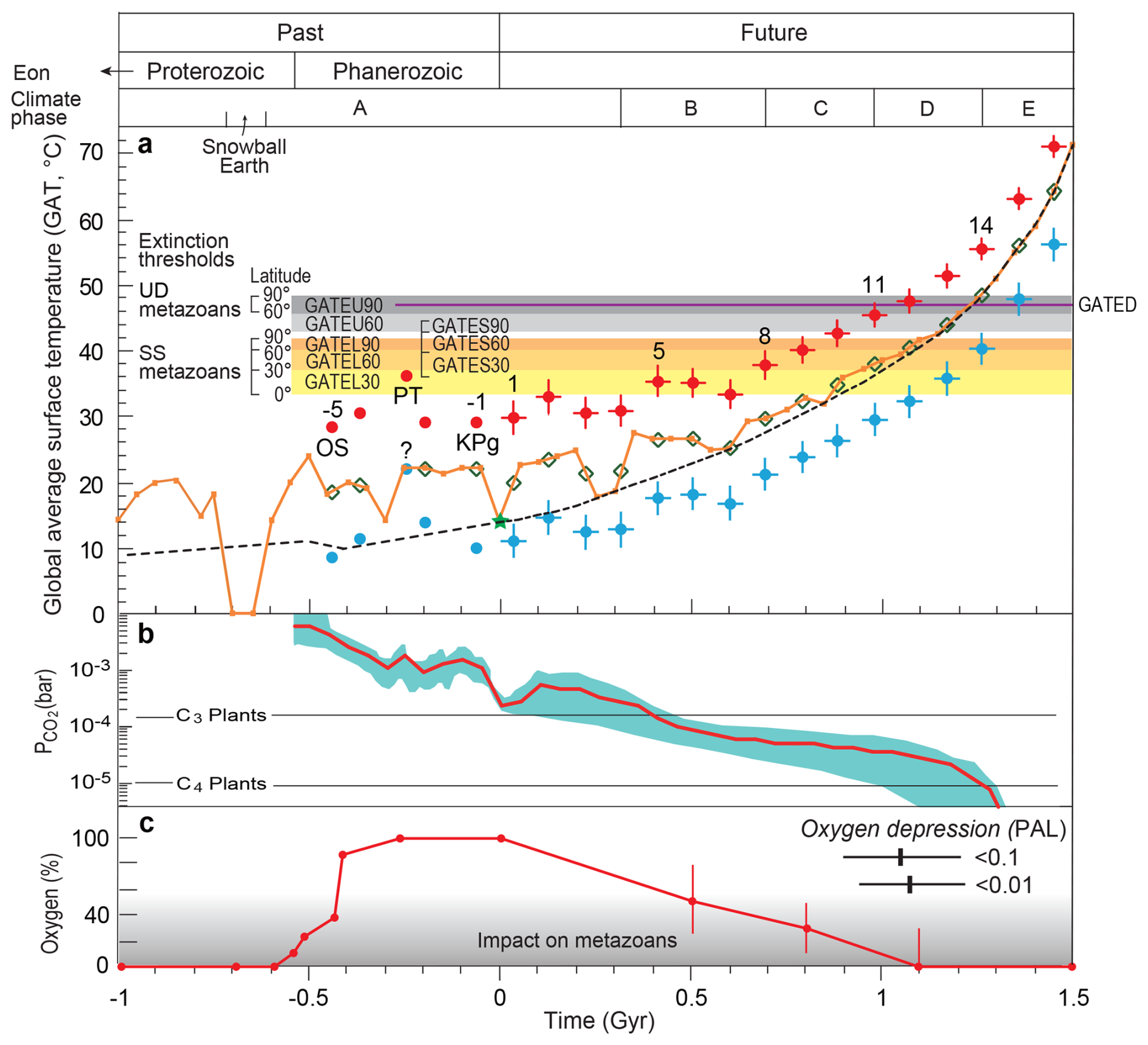
Figure 2 Global average surface temperature and atmospheric CO₂ and oxygen levels over the past and future 2.5 Gyr. Global average surface temperature (a), CO₂ content (b), and atmospheric oxygen levels (c) are shown for the past 1.0 billion years (−1.0 Gyr) and projected for the next 1.5 Gyr (to +1.5 Gyr), together with metazoan extinction thresholds and climate phases. The black dashed line, adapted from Mello and Friaça (2019), represents long-term historical trends (error range: −0.1 to +0.2 Gyr). The orange curve illustrates long-term cyclical icehouse–greenhouse variations (error range: ±0.1 Gyr), based on historical data from Scotese et al. (2021) and estimates for −1.0 to −0.6 Gyr from Vérard (2024) (Table S1). Future projections for both curves begin at the green star marking the modern global average temperature (14 °C). The future portion of the orange curve is calculated from CO₂ content data (b; Table S1).
Light blue and red dots indicate average surface temperatures during major mass extinction events, representing cooling phases (blue) and subsequent warming phases (red) (Kaiho, 2025; Table S2). Green open diamonds show temperatures immediately preceding each extinction. Vertical error bars denote the standard deviations of temperature anomalies associated with major extinction events (Table S2).
The yellow–orange shaded regions (corresponding to open circles in Fig. 4) represent upper temperature limits for superterranean and surface-water (SS) metazoan extinction across three latitude bands (0–30°, 30–60°, 60–90°) (GATEL and GATES). Gray shaded regions mark extinction thresholds for subterranean (U) metazoans at 30–60° and 60–90° (GATEU). The extinction threshold for deep-sea (D) metazoans is indicated by the purple horizontal line (GATED; see Fig. 4). “PT” and “KPg” denote the Permian–Triassic and Cretaceous–Paleogene boundary events, while numbers −5, −1, 1, 5, 8, 11, and 14 correspond to event identifiers. Predicted timings of future atmospheric CO₂ and oxygen depletion follow Ozaki and Reinhard (2021). The gray gradient in panel (c) indicates the magnitude of oxygen-related constraints on metazoan diversity (see Eqs. 21 and 22 in Sect. 2.5), with darker shading indicating stronger limitations. PAL refers to Present Atmospheric Level. Past atmospheric oxygen data are from Krause et al. (2018) and Sperling et al. (2015).

I selected the five major mass extinctions, each marked by abrupt environmental disruption and >35 % marine genera loss – equivalent to >60 % species extinction – based on Raup and Sepkoski (1982), Bambach (2006), and Kaiho (2022a). Family-level extinction percentages capture severe biodiversity losses across taxa. Insects experienced 35 %, 14 %, and 8 % family-level extinction across the same events (Table S3 in the Supplement; Labandeira and Sepkoski, 1993). Terrestrial tetrapod family-level extinctions were 54 %, 21 %, and 38 % at the end-Permian, end-Triassic, and end-Cretaceous, respectively (Table S4 in the Supplement; Benton, 2010). Marine metazoan family-level extinctions were ∼22 % (end-Ordovician), 21 % (Late Devonian), 50 % (end-Permian), 20 % (end-Triassic), and 15 % (end-Cretaceous) (Table S5 in the Supplement; Sepkoski, 1982). Because terrestrial tetrapods and insects originated shortly before the second mass extinction, diversity data are unavailable for the first two events.

Global temperature anomalies associated with each extinction event follow Kaiho (2022a, 2024, 2025), based on data from Finnegan et al. (2011), Balter et al. (2008), Huang et al. (2018), Chen et al. (2016), Korte et al. (2009), and Vellekoop et al. (2014). Most of these extinctions were triggered by large-scale volcanism, except the end-Cretaceous event, which was caused by an asteroid impact (Kaiho, 2025).

Although climate cycles evolve over long timescales, mass extinctions unfold far more abruptly. Both processes contribute to global warming and may therefore shorten the time remaining before the eventual disappearance of metazoans in the distant future.

Projections of future atmospheric O₂ levels and marine and terrestrial biodiversity were guided by patterns observed during the Paleozoic biodiversity maximum. In the early Ediacaran (∼0.6 Gyr), atmospheric O₂ was ∼0.01 PAL, while marine metazoan diversity rate for the Paleozoic maximum was ∼0.04 (family level). O₂ increased to ∼0.10 PAL (diversity rate=0.2) by the late Ediacaran (∼0.55 Gyr), to ∼0.24 PAL (diversity rate=0.4) during the Cambrian Explosion (∼0.52 Gyr), and reached ∼0.38 PAL (diversity rate=1.0) by the end-Ordovician (∼0.44 Gyr). Atmospheric O₂ further rose to ∼0.86 PAL, with diversity remaining at ∼1.0 by the end-Silurian (∼0.42 Gyr). Fossil evidence indicates that terrestrial metazoans (insects and tetrapods) first appeared when atmospheric O₂ levels approached ∼0.8 PAL (Fig. 3). Although these estimates carry substantial uncertainty, they follow the reconstructions of Krause et al. (2018, 2022), supported by Sperling et al. (2015) (Fig. 2c, Table 1).

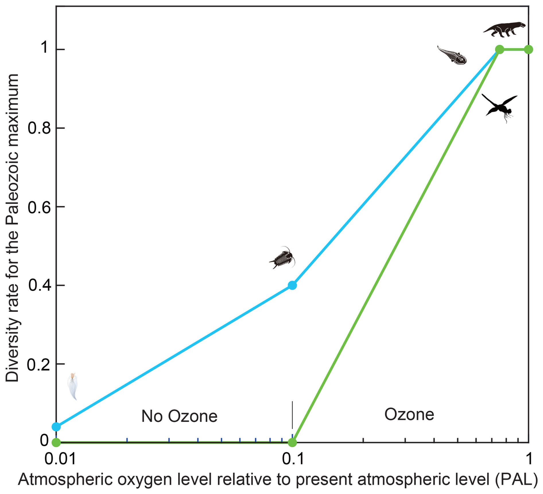
Figure 3 Relationship between atmospheric oxygen levels and past metazoan diversity. This figure illustrates the relationship between atmospheric oxygen concentrations and the diversity of marine metazoans, terrestrial tetrapods, and insects. Blue lines with circular markers show marine metazoan diversity, while pale green lines with square markers represent terrestrial tetrapods and insects. Data span the Neoproterozoic and Paleozoic intervals during which atmospheric oxygen rose substantially. Oxygen level estimates are from Sperling et al. (2015) and Krause et al. (2022), and diversity data derive from Erwin et al. (1987), Labandeira and Sepkoski (1993), Engel and Grimaldi (2004), and Benton (2010). Silhouettes of metazoans depict approximate diversity levels and associated oxygen concentrations.

Table 1 Atmospheric oxygen levels and metazoan diversity rates controlled by oxygen from −1 to 1.5 Gyr.

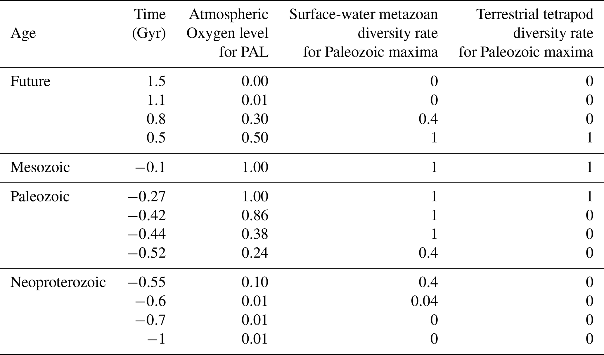
Past atmospheric oxygen levels (in PAL) are compiled from Krause et al. (2022) and Sperling et al. (2015), while future oxygen levels are based on projections by Ozaki and Reinhard (2021). Future metazoan diversity rates are estimated from the empirical relationship between atmospheric oxygen levels and metazoan diversity observed in the geological record (Fig. 3). Superterranean metazoan diversity rates in the future are inferred from terrestrial plant diversity trends during the Silurian–Carboniferous interval, reflecting the evolutionary lag between terrestrial plant diversification and the subsequent rise of terrestrial tetrapods (Cascales-Miñana, 2016). PAL = Present Atmospheric Level.

The following section uses the positive correlation between atmospheric O₂ and biodiversity to constrain future projections, highlighting that the emergence and diversification of terrestrial metazoans occurred during intervals of elevated oxygen levels.

2.3 Future temperature projections

A coherent framework for projecting future global temperatures is illustrated in Fig. 1 (highlighted in pale red, yellow, and green). Surface temperature estimates were generated using long-term warming trends, cyclical climate variations, and abrupt events (Events 1–16, modeled as analogs to the “Big Five” mass extinctions), following Eqs. (1)–(7) in this subsection. Mantle temperature is treated as a key control on abrupt events (Eqs. 4–7). The same pacing of icehouse–greenhouse cycles (∼0.3 Gyr intervals) and major abrupt extinction events (∼0.094 Gyr intervals) is applied to future climate projections. The uncertainties associated with these cyclicities provide estimates for the timing of complete metazoan extinction, with error margins of ±0.1 Gyr for climate cycles and ±0.03 Gyr (standard deviation for “Big Five” mass extinction numerical ages) for abrupt event timing.

To project future global temperatures, I compiled Global Average Temperature (GAT) data spanning 2.5 Gyr – including the past 1.0 Gyr (Mello and Friaça, 2019; Scotese et al., 2021; Kaiho, 2022a) and the projected next 1.5 Gyr – and integrated both reconstructed historical variations and future projections (orange curve and red/blue points in Fig. 2). Three major physical drivers were incorporated: long-term solar-driven warming, cyclical climate rhythms, and abrupt climate events.

The GAT is calculated as:

$$\begin{array}{}\text{(1)}& \text{GAT}=\text{Ts}+\mathrm{\Delta }\text{Tc}+\mathrm{\Delta }\text{Te}\end{array}$$

where Ts is the long-term warming trend mainly driven by increasing solar luminosity; ΔTc is the temperature anomaly associated with climate cycles; and ΔTe is the anomaly associated with abrupt events.

Ts is based on the long-term thermal evolution model of Mello and Friaça (2019), consistent with Franck et al. (2006) and Wolf et al. (2017).

ΔTc is set to a maximum of 8 °C during greenhouse intervals, gradually decreasing to 0 °C by 1.2 Gyr and remaining low thereafter, while icehouse intervals are set to 0 °C. The 8 °C anomaly reflects the icehouse–greenhouse contrast reconstructed for the Phanerozoic (Scotese et al., 2021). The gradual decrease is attributed to decreasing CO₂ caused by enhanced continental weathering under increasing solar luminosity. Earth's past climate exhibits 0.35–0.30 Gyr periodicity (Fig. 2) composed of ∼0.2 Gyr greenhouse and ∼0.1 Gyr icehouse intervals (Scotese et al., 2021; Torsvik et al., 2024; Vérard, 2024).

ΔTc values were further refined using the well-established 1.5–4 °C warming expected from CO₂ doubling (Sherwood et al., 2020). Starting from the present 14 °C global temperature, all future variations were projected (Table S1; orange curve in Fig. 2). Although future climatic periodicity may shift due to mantle cooling and increased solar flux, the maximum uncertainty in diversity-phase timing is limited to ∼0.1 Gyr, a minor effect because CO₂ decline increasingly suppresses cyclic temperature anomalies.

Temperature anomalies associated with abrupt events were estimated from average values of the five major extinction events, excluding the Permian–Triassic cooling whose magnitude remains uncertain (Kaiho, 2025). These anomalies decrease through time owing to reduced mantle temperatures and correspondingly reduced CO₂ and SO₂ emissions.

Short-lived (<10 kyr) temperature anomalies substantially affect climate despite their minimal influence on long-term trends. These anomalies are defined as cooling followed by warming (light blue and red points in Fig. 2) based on global SST reconstructions (Kaiho, 2022a).

The magnitudes of ΔTe were calculated using experimental data (Kaiho et al., 2022a; Kaiho, 2025) and mantle-dependent emission rates, following:

$$\begin{array}{}\text{(2)}& {\displaystyle }\mathrm{\Delta }\text{Te}=-\mathrm{8.9}-(-\mathrm{8.9}+\mathrm{8.9}\times \text{SR})\times \mathrm{2}/\mathrm{3}\left[\text{cooling cases}\right]\text{(3)}& {\displaystyle }\mathrm{\Delta }\text{Te}=\mathrm{9.9}\times \text{CR}\left[\text{warming cases}\right]\end{array}$$

where −8.9 and +9.9 °C are the mean cooling and warming anomalies of past mass extinctions. SR and CR are the relative SO₂ and CO₂ emission rates derived from mantle-temperature–dependent regressions:

$$\begin{array}{}\text{(4)}& {\displaystyle }\text{SR}=(\mathrm{0.00108}\text{Ts}-\mathrm{0.236})/\mathrm{42.25}(r=\mathrm{0.97})\text{(5)}& {\displaystyle }\text{CR}={\displaystyle \frac{(\mathrm{0.501}\times p)}{\mathrm{0.348}}},p=e^{\mathrm{0.0077}{T}_{\text{sill}}}(r=\mathrm{0.90})\end{array}$$

The sill temperature after 100 years is calculated by:

$$\begin{array}{}\text{(6)}& T_{\text{sill}}=(E\times \text{Ti})/(E-\text{Ti}\times \ln t_{\mathrm{i}}/t_{\mathrm{s}})\end{array}$$

and initial sill (a tabular sheet intrusion from magma) temperature:

$$\begin{array}{}\text{(7)}& \text{Ti}=\text{Tm}\times \mathrm{1423}/\mathrm{1603}\end{array}$$

Where T_m is mantle temperature, E is activation energy (74 kcal mol⁻¹ for CO₂ release, Jackson et al., 1995, and 67 kcal mol⁻¹ for SO₂, Concer et al., 2017), t_s and t_i are heating durations, and 1423–1603 K represent typical sill and mantle temperatures. The modern mantle temperature is 1603 K (Mello and Friaça, 2019), and the average initial sill temperature is 1423 K (Aarnes et al., 2010); the 180 K difference reflects typical cooling during sill formation. Equations (4) and (5) represent best-fit curves derived from the heating experiments of Kaiho et al. (2022) and Kaiho (2024). Equation (6) is from the Arrhenius equation on page 174 of IUPAC (1996).

The above ΔTe is in the mean temperature anomaly case. When accounting for mantle temperature, warming anomalies in the maximum and minimum temperature anomaly cases are 3 °C higher and 2 °C lower, respectively, than the anomaly in the mean temperature anomaly case, 0.7–1.1 Gyr (events 8–12) from now (Table S2). These differences are 4 °C higher and 3 °C lower, respectively, when based on modern mantle temperature (Table S2).

2.4 Metazoan thermal tolerance limits

The upper thermal tolerance limits of terrestrial ectotherms (e.g., amphibians, reptiles, arthropods) range from approximately 45–47 °C in low–mid latitudes (0–60°) and decline to 35–40 °C in high latitudes (60–90°) (Sunday et al., 2011; Araújo et al., 2013). Marine ectotherms (e.g., mollusks, fish, crustaceans) exhibit upper limits of 40–45 °C between 35° N and 50° S, decreasing substantially to 10–20 °C toward polar regions (Sunday et al., 2011). Although cold tolerance shows wide variability, upper thermal tolerance tends to be phylogenetically conserved among both ectotherms and endotherms (Araújo et al., 2013).

Across metazoans, temperatures exceeding 45–47 °C on land, 40–45 °C in surface oceans, and 42–46 °C across most marine and terrestrial habitats approach the limits at which metabolic processes, protein stability, and membrane integrity begin to fail (Somero, 1995; Pörtner, 2002). These thresholds represent the approximate upper bounds for sustained metazoan survival. In this study, a metazoan species was assumed to go extinct at any latitude if the monthly mean of daily maximum temperatures in the warmest month at its habitat exceeded 46 °C.

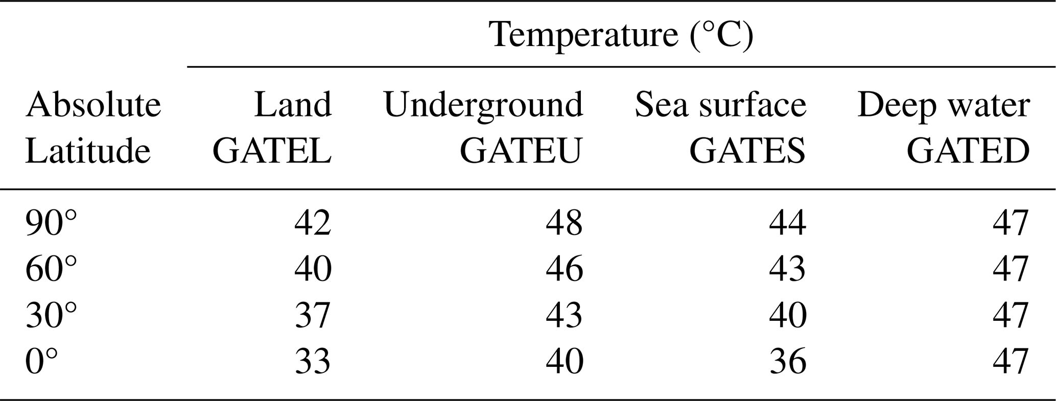
Using these physiological limits, extinction threshold temperatures were calculated for four major habitat categories – superterranean (St), subterranean (Ut), surface-water (Sw), and deep-water (Dw) metazoans – across all latitude zones (Fig. 4). These thresholds provide essential constraints for projecting how rising global temperatures will affect the persistence of metazoan life in different ecological environments.

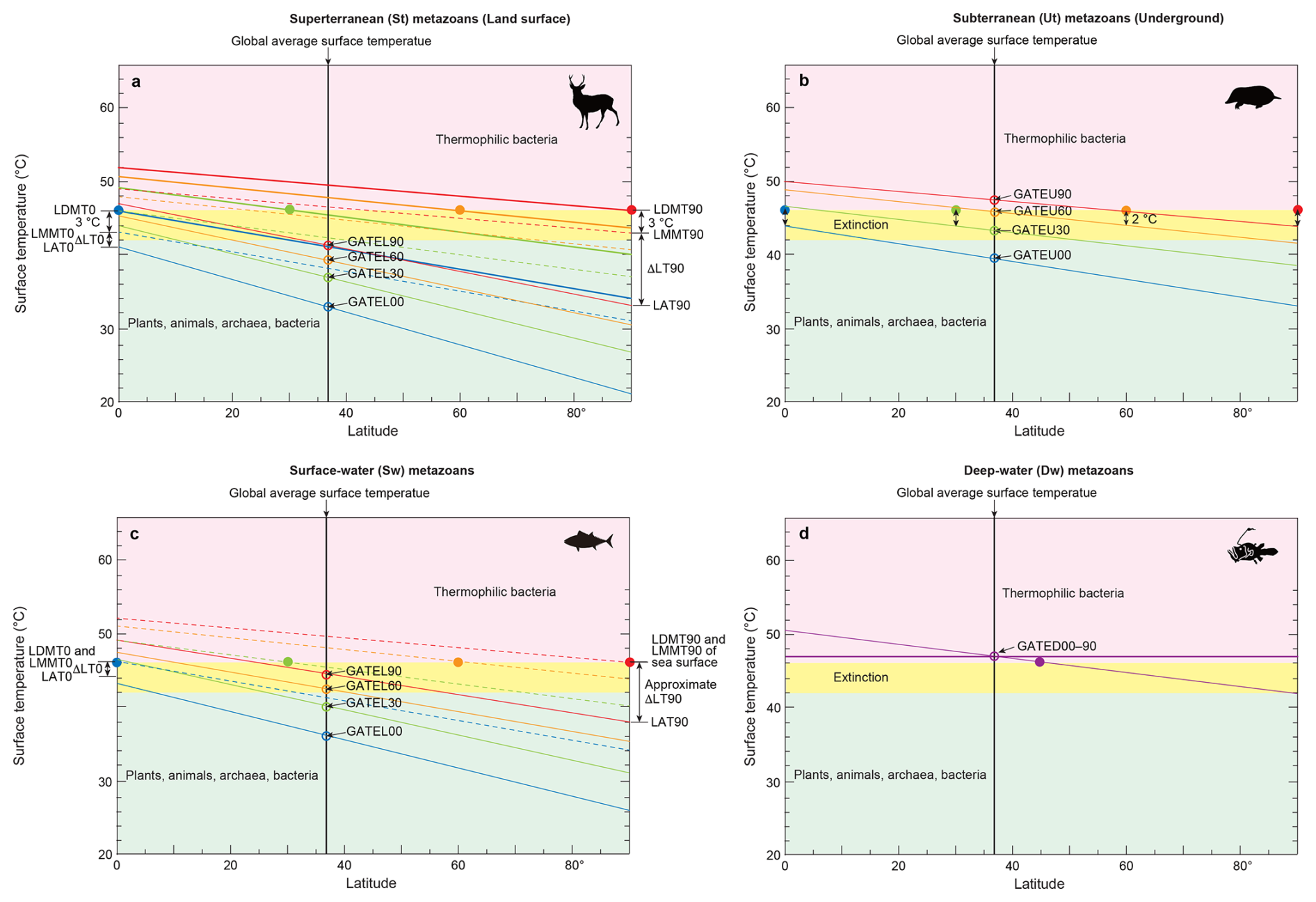
Figure 4 Surface temperatures across latitudes corresponding to the extinction thresholds of four metazoan groups. (a) Global Average surface Temperature (GAT) required for the extinction of superterranean (St; surface-dwelling terrestrial) metazoans (GATEL). Thick oblique lines represent Local Daytime Maximum Temperatures during the warmest month (LDMT). Dashed oblique lines indicate Local Monthly Maximum Temperatures (LMMT), and thin oblique lines indicate Local Average Temperatures (LAT). LT = Local Temperature. Latitudes 0, 30, 60, and 90° are labeled as 00, 30, 60, and 90, respectively. The intersection of the vertical black line at 37° with LAT oblique lines yields the global average surface temperatures GATEL00 to GATEL90. (b) GAT required for the extinction of subterranean (Underground) metazoans (GATEU). (c) GAT required for the extinction of surface-water (Sw) marine metazoans (GATES). (d) GAT required for the extinction of deep-water (Dw) metazoans (GATED). The purple horizontal line represents the upper thermal threshold for deep-water metazoans. Across all panels (a)–(d), the yellow-shaded region denotes the temperature range capable of causing metazoan extinction, common to both terrestrial and marine groups (Sunday et al., 2011; Araújo et al., 2013). Closed circles mark the maximum extinction temperature (46 °C) at latitudes 0, 30, 60, and 90°. Corresponding open circles, color-matched to the closed markers, indicate the global average temperatures associated with these extinction thresholds. See Methods Sect. 2.4 for details.

2.4.1 For superterranean (St) metazoans

The extinction thresholds for superterranean (St) metazoans – surface-dwelling terrestrial animals – were estimated using the temperature framework illustrated in Fig. 4a. Oceanic climate regions on land were used as reference points because they experience milder and more stable climates than continental interiors. The Global Average surface Temperature at Extinction (GATE) for St (surface of Land) metazoans (GATEL; Fig. 2a) was determined through the following steps:

• 1.

  Upper thermal tolerance definition
  The upper survival limit for St metazoans is set to 46 °C, corresponding to the average Local Daily Maximum Temperature (LDMT) in warm-month oceanic climate zones at 0, 30, 60, and 90° latitude.

• 2.

  Use of coastal temperature records
  Coastal climate data were selected because maximum daily temperatures in coastal areas are generally lower than in inland regions, providing a conservative estimate for lethal conditions (dashed oblique lines in Fig. 4).

• 3.

  Conversion from LDMT to Local Monthly Maximum Temperature (LMMT)
  A −3 °C correction was applied to convert LDMT to LMMT. This offset reflects the typical difference between monthly mean and daily maximum temperatures during the warmest month, based on observations from coastal cities including Singapore (∼0° N), Shanghai (∼30° N), Helsinki (∼60° N), and Longyearbyen (∼80° N) (Weather Spark).

• 4.

  Conversion from LMMT to Local Annual Temperature (LAT)
  LAT was derived by applying a latitudinally dependent correction (ΔLT; Fig. 4). ΔLT values were set to −2, −3.5, −7.5, and −9 °C for ∼0, ∼30, ∼60, and ∼80° N, respectively, following temperature differences observed in coastal cities of the eastern Atlantic (Weather Spark).

• 5.

  Establishing warm-Earth latitudinal temperature gradients
  The warm-Earth latitudinal gradient of LAT was set to be 20 and 14 °C larger than the corresponding sea-surface temperature (SST) gradients of 17 and 11 °C from 0 to 90° latitude when GAT is 30 and 40 °C, respectively (thin oblique lines in Fig. 4a; Gaskella et al., 2022). These gradients reflect changes in solar incidence associated with Earth's axial tilt.

Common procedure for all metazoan groups

• 6.

  Determine GATE from LAT at a representative latitude
  LAT at 37° absolute latitude was used as a proxy for Global Annual Temperature (GAT), because modern GAT (14 °C) closely matches LAT at 37° N in oceanic climate regions (Iwaki and San Francisco; Weather Spark).

• 7.

  Calculate extinction thresholds (GATE values)
  GATEL (land), GATES (surface water), GATEU (underground), and GATED (deep water) were derived from LAT at 37°, as shown by open dots in Fig. 4.

• 8.

  Plot extinction latitudes
  Resulting extinction latitudes (e.g., GATEL30) are illustrated in Fig. 2a.

The LAT required to induce extinction of St metazoans at each latitude (0, 30, 60, 90°) is calculated using:

$$\begin{array}{}\text{(8)}& \text{LAT}=\mathrm{46}-\mathrm{3}-\mathrm{\Delta }\text{LT}\left(\mathrm{°}\mathrm{C}\right)\end{array}$$

where ΔLT is the latitude-dependent correction applied when converting LMMT to LAT.

2.4.2 Subterranean (underground) metazoans (Ut)

The extinction thresholds for subterranean metazoans (GATEU) were determined using Fig. 4b. Although most modern subterranean organisms inhabit shallow depths (∼10 cm), future subterranean metazoans capable of tolerating elevated surface temperatures are expected to retreat to depths of approximately 2.5 m. At this depth, the temperature difference between the Local Monthly Maximum Temperature (LMMT) and the Local Annual Temperature (LAT) is about 2 °C – low enough to allow survival. In contrast, at a depth of 1 m this difference approaches ∼8 °C, which is too large for survival (Singh and Sharma, 2017). At depths ≥4 m, soil temperature becomes nearly constant throughout the year. The difference between LDMT and LMMT is less than 1 °C (Singh and Sharma, 2017). In Fig. 4b, oblique LAT lines were therefore plotted 2 °C below the closed 46 °C points, representing lethal thermal limits, for subterranean animals living at a depth of 2.5 m. The warm-Earth latitudinal gradient of LAT was set to be sea-surface temperature (SST) gradients of 11 and 5 °C from 0 to 90° latitude when GAT is 40 and 50 °C, respectively (thin oblique lines in Fig. 4c; Gaskella et al., 2022).

2.4.3 Surface-water (Sw) metazoans

In the surface ocean, the difference between LDMT and LMMT is less than 1 °C; therefore, the sea-surface LMMT is assumed to equal the LDMT used for land. As a result, extinction thresholds for surface-water metazoans (GATES) are set 3 °C higher than those for terrestrial superterranean metazoans (GATEL), as shown in Fig. 4c. The warm-Earth latitudinal gradient of LAT was set to be sea-surface temperature (SST) gradients of 17 and 11 °C from 0 to 90° latitude when GAT is 30 and 40 °C, respectively (thin oblique lines in Fig. 4c; Gaskella et al., 2022).

2.4.4 Deep-water (Dw) metazoans

Deep-sea temperatures remain highly stable year-round, and therefore Fig. 4d does not require multiple oblique LAT lines. Deep-water temperatures were derived from annual surface temperatures at 45° absolute latitudes. The reference extinction threshold is represented by the purple closed circle at 45° latitude (46 °C) in Fig. 4d. The resulting deep-water extinction threshold (GATED) corresponds to a global surface temperature of 47 °C, shown by the purple open circle in Fig. 4d.

2.5 Integrated future diversity model using temperature, oxygen, and CO₂

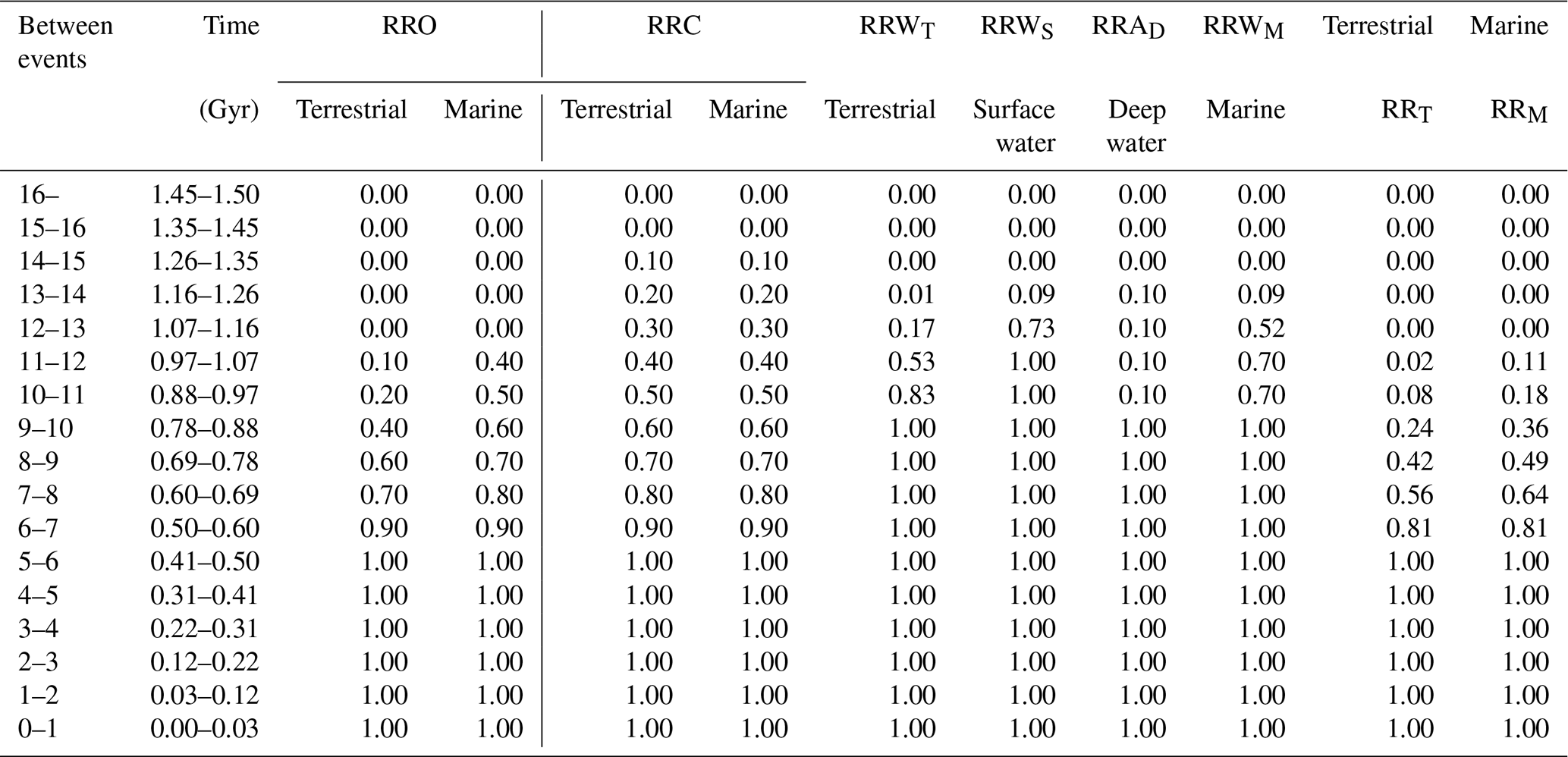
The future diversity model consists of alternating extinction events and recovery phases (Tables 2–4), synthesized from data in Tables 1 and 4–8. Extinction events include climate-driven crises and food scarcity occurring after the disappearance of surface-dwelling metazoans. Each event leads to substantial biodiversity loss, while recovery phases restore diversity to varying extents depending on environmental conditions. Prior to the onset of the C₃ plant crisis, recovery rates (referring to completeness, not speed) are set to 1.0, indicating full biodiversity recovery. However, once the C₃ plant crisis begins, recovery rates gradually decline as atmospheric CO₂ and O₂ levels drop, reducing ecosystem resilience and limiting the potential for complete recovery.

Table 2 Extinction and recovery model for future projections, showing survival rates at the family level under the Conservative Model – average extinction rate case.

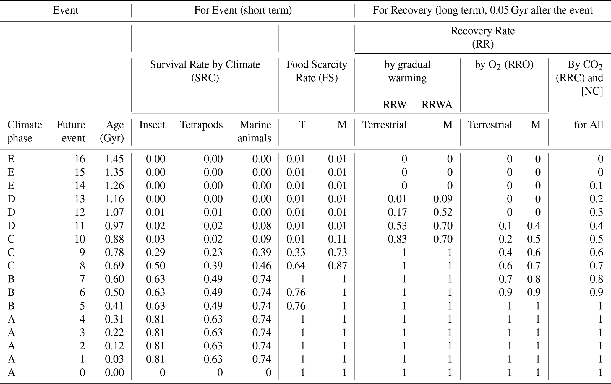
Survival rates of 0.63 (terrestrial tetrapods), 0.81 (insects), and 0.74 (marine animals) are derived from fossil-based estimates in Tables S3–S5. All other survival rates are obtained from the methodological framework described in Sect. 2.5. Event 0 represents the Anthropogenic Crisis. Future survival rates for insects are scaled from those of tetrapods using the ratio $\mathrm{0.81}/\mathrm{0.63}$. T: Terrestrial. M: Marine.

The calculation procedure is as follows.

First, the modern diversity (i.e., number of families) at time 0 for each metazoan group is multiplied by the survival rate (referring to completeness, not speed) for each extinction event in the three models (Conservative Model, New Evolutional Model, and Continuous Worst Anthropocene Model; Tables 2–4), yielding the post-event diversity (Event 0 [0E]) (Table S6 in the Supplement).

Second, the post-event diversity is multiplied by the corresponding recovery rate to calculate the diversity 0.05 Gyr after the event (0R). For Event 0, a special case is applied using 0.03 (or 0.029) Gyr, since Event 1 occurs at that time. The value at 0R is then carried forward unchanged until immediately before the next event, referred to as 0A. Although 0R and 0A occur at the same time, there is an effective 0.05 Gyr interval between E (event) and R (recovery), as well as between R and A (aftermath). A and the next E share the same time point, but A is considered just before the event.

Third, the diversity at time 0A is multiplied by the appropriate survival rate to determine the diversity at time 1E. This process is repeated sequentially for Events 1–16 to project biodiversity trends from the present to 1.5 Gyr into the future (Table S6), using Eqs. (9)–(22).

Average, maximum, and minimum family-level extinction percentages derived from past mass extinctions were used to project future biodiversity change (Table S6). When the GATEL exceeds 37 °C (GATEL30) – the threshold at which low-latitude (0–30°) regions become uninhabitable (Fig. 2a) – survival rates are further adjusted using the Extinction Area Rate (EAR [km² km⁻²]) and family-level diversity rate across each latitude (DRL). Major drivers of past mass extinctions include global cooling, global warming, ozone-layer destruction that exposes organisms to harmful short-wavelength UV radiation, ocean acidification, and widespread oceanic anoxia. Under future solar-luminosity-driven warming, prolonged high GAT adds an additional extinction pressure to the baseline values derived from past events (Eq. 15). After all surface-dwelling metazoans disappear, diversity is further reduced by applying the Food Scarcity Rate (FS), reflecting the restriction of ecosystems to deep-sea chemosynthetic and subterranean habitats (Eq. 9).

Future diversity trajectories are influenced by several interacting processes: the ongoing anthropogenic crisis (Event 0), subsequent abrupt mass-extinction analogs (Events 1–11), the sequential C₃ and C₄ plant crises driven by progressive CO₂ depletion, and the long-term decline in atmospheric oxygen (Fig. 2b and c, Tables 2–4). The C₃ plant crisis is defined at ∼0.15 mbar CO₂ and the C₄ plant crisis at ∼0.01 mbar CO₂ (Fig. 2b). Enhanced continental weathering under warming causes the C₃ plant crisis to begin gradually at 0.4 Gyr and the C₄ crisis at 1.0–1.3 Gyr. These collapses trigger metazoan extinction events of ∼40 % at 0.9 Gyr and nearly 100 % between 0.9 and 1.3 Gyr.

Diversity for each event and recovery interval is calculated as (Table 5):

$$\begin{array}{}\text{(9)}& {\displaystyle }{D}_{\text{nE}}=D_{(n-\mathrm{1})A}\times {\text{SRC}}_n\times {\text{FS}}_n\left[\text{for events}\right]\text{(10)}& {\displaystyle }{D}_{\text{nR}}=D_{(n-\mathrm{1})A}\times \text{RR}\left[\text{for recovery periods}\right]\end{array}$$

For Events 1–16, Survival Rate by Climates for insects (SRC_I), tetrapods (SRC_T), and marine metazoans (SRC_M) are derived as:

Table 3 Extinction and recovery model for future projections, showing family-level survival rates under the New Evolutional Model – average extinction rate case.

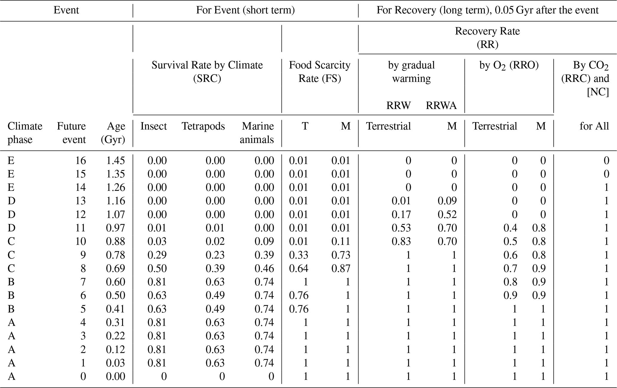
This model incorporates adaptive evolution to extremely low atmospheric O₂ and CO₂ levels. Survival rates are derived from Sect. 2.5 and Table S5. T: Terrestrial. M: Marine.

Average Extinction Rate Case
(Family-level extinction rates: 0.19 for insects, 0.37 for tetrapods, 0.26 for marine metazoans):

$$\begin{array}{}\text{(11a)}& {\displaystyle }{\mathrm{\text{SRC}}}_{\mathrm{I}}=\mathrm{1}-(\mathrm{0.19}+\mathrm{0.77}\times {\text{ERW}}_{\text{SI}}+\mathrm{0.04}\times {\text{ERW}}_{\mathrm{U}})\text{(12a)}& {\displaystyle }{\mathrm{\text{SRC}}}_{\mathrm{T}}=\mathrm{1}-(\mathrm{0.37}+\mathrm{0.60}\times {\text{ERW}}_{\text{ST}}+\mathrm{0.03}\times {\text{ERW}}_{\mathrm{U}})\text{(13a)}& {\displaystyle }{\mathrm{\text{SRC}}}_{\mathrm{M}}=\mathrm{1}-(\mathrm{0.26}+\mathrm{0.50}\times {\text{ERW}}_{\text{SM}}+\mathrm{0.24}\times {\text{ERWA}}_{\mathrm{D}})\end{array}$$

Maximum Extinction Rate Case
(Family-level extinction rates: 0.35, 0.54, 0.35):

$$\begin{array}{}\text{(11b)}& {\displaystyle }{\mathrm{\text{SRC}}}_{\mathrm{I}}=\mathrm{1}-(\mathrm{0.35}+\mathrm{0.62}\times {\text{ERW}}_{\text{SI}}+\mathrm{0.03}\times {\text{ERW}}_{\mathrm{U}})\text{(12b)}& {\displaystyle }{\mathrm{\text{SRC}}}_{\mathrm{T}}=\mathrm{1}-(\mathrm{0.54}+\mathrm{0.44}\times {\text{ERW}}_{\text{ST}}+\mathrm{0.03}\times {\text{ERW}}_{\mathrm{U}})\text{(13b)}& {\displaystyle }{\mathrm{\text{SRC}}}_{\mathrm{M}}=\mathrm{1}-(\mathrm{0.35}+\mathrm{0.44}\times {\text{ERW}}_{\text{SM}}+\mathrm{0.31}\times {\text{ERWA}}_{\mathrm{D}})\end{array}$$

Minimum Extinction Rate Case
(Family-level extinction rates: 0.08, 0.21, 0.15):

$$\begin{array}{}\text{(11c)}& {\displaystyle }{\mathrm{\text{SRC}}}_{\mathrm{I}}=\mathrm{1}-(\mathrm{0.08}+\mathrm{0.87}\times {\text{ERW}}_{\text{SI}}+\mathrm{0.05}\times {\text{ERW}}_{\mathrm{U}})\text{(12c)}& {\displaystyle }{\mathrm{\text{SRC}}}_{\mathrm{T}}=\mathrm{1}-(\mathrm{0.21}+\mathrm{0.75}\times {\text{ERW}}_{\text{ST}}+\mathrm{0.04}\times {\text{ERW}}_{\mathrm{U}})\text{(13c)}& {\displaystyle }{\mathrm{\text{SRC}}}_{\mathrm{M}}=\mathrm{1}-(\mathrm{0.15}+\mathrm{0.57}\times {\text{ERW}}_{\text{SM}}+\mathrm{0.28}\times {\text{ERWA}}_{\mathrm{D}})\end{array}$$

Note: ERW (extinction rate by warming) is calculated based on the mean, maximum, and minimum temperature anomaly scenarios.

The ERW coefficients are calculated as follows:

• For terrestrial metazoans, a coefficient of 0.05 represents the proportion of subterranean families (15 out of 315), based on mammalian lineage data (Recknagel and Trontelj, 2021; Benton, 2010), while the remaining 0.95 corresponds to surface-dwelling families.

• For marine metazoans, a coefficient of 0.33 reflects the proportion of deep-sea fish families among all marine fish families. This is based on approximately 6 % of teleost species (which make up the majority of all fish) being restricted to depths greater than 200 m (Miller et al., 2022), scaled using the species–genus–family extinction relationship (Kaiho, 2022a). The remaining 0.67 applies to surface-water taxa.

The diversity of superterranean and subterranean metazoans changes independently due to global average temperature (GAT), while the diversity of surface-water and deep-water marine organisms is influenced independently by both high GAT and low dissolved oxygen, as described in Eqs. (11)–(13) (Fig. 2).

The survival rate (SR) and recovery rate (RR) represent changes in family-level diversity, calculated relative to modern values: 610 insect families, 315 tetrapod families, and 950 marine metazoan families. For Event 0, SR values are set at 0.95 (insects), 0.80 (tetrapods), and 0.90 (marine metazoans), based on extinction data from Kaiho (2026) and Fig. 1 of Kaiho (2022a).

• Average extinction rate case: 0.19 (insects), 0.37 (tetrapods), and 0.26 (marine metazoans), representing the average family-level extinction rates during past major mass extinctions.

• Maximum extinction rate case: 0.35, 0.54, and 0.35, representing the highest observed family-level extinction rates.

• Minimum extinction rate case: 0.08, 0.21, and 0.15, representing the lowest observed family-level extinction rates.

(See Tables S3–S5.)

These average, maximum, and minimum extinction rates are used to estimate the potential magnitude of future extinctions, enabling exploration across a broader range of extinction scenarios.

Importantly, mass extinctions are caused not only by global warming but also by reductions in sunlight due to stratospheric aerosols, which induce global cooling, along with decreases in precipitation. Accordingly, the total extinction rate for each metazoan group is treated as the sum of the past major mass-extinction rate and the additional extinction rate attributable specifically to global warming during future intervals in which excess LDMT conditions exceed 46 °C.

$$\begin{array}{}\text{(14)}& \text{ERW}=\text{EAR}\times \text{DRL}\end{array}$$

DRL is the family-level Diversity Rate transformed from generic diversity across each latitude band for terrestrial mammals based on 193 km×193 km grid cells (Li et al., 2021) using the method of Kaiho (2022a). Calculations of ERW_ST, ERW_SI, and ERW_SM are provided in Table 5.

Table 4 Extinction and recovery model for future projections, showing family-level survival rates under the Continuous Worst Anthropocene Model – average extinction rate case, which assumes persistent anthropogenic pressures extending to the end of metazoans.

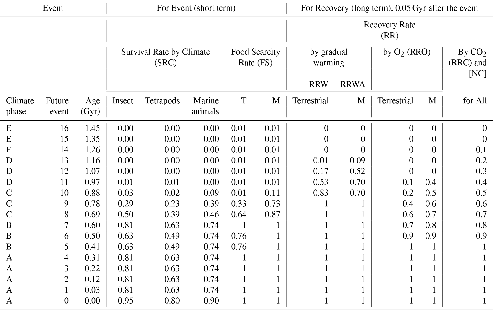
Survival rates are sourced from Sect. 2.5 and Table S5. T: Terrestrial. M: Marine.

ERWA_D, the extinction rate due to warming and anoxia for marine groups, is defined as:

$$\begin{array}{}\text{(15)}& \begin{array}{rl}& \text{GAT}<\mathrm{36}\mathrm{°}\mathrm{C}(\text{events 1–4, 7):}{\text{ERWA}}_{\mathrm{D}}=\mathrm{0}\\ & \begin{array}{rl}\text{GAT}\ge \mathrm{36}\mathrm{°}\mathrm{C}(& \text{events 5, 6, 8–11):}\\ & {\text{ERWA}}_{\mathrm{D}}=\mathrm{0.9}\left(\text{anoxia-driven}\right)\end{array}\\ & \begin{array}{rl}\text{GAT}\ge \mathrm{48}\mathrm{°}\mathrm{C}(& \text{events 12–16):}\\ & {\text{ERWA}}_{\mathrm{D}}=\mathrm{1}\left(\text{warming-driven}\right)\end{array}\end{array}\end{array}$$

ERWA is applied only to deep-water metazoans. Relevant temperature thresholds are based on Permian-Triassic deep-ocean extinction conditions.

Food Scarcity Rate (FS) is set as Survival Rate in Tables 2–4 using GAT of GATEL and GATES in Fig. 2a, because the food resources of subterranean and deep-sea metazoans are largely derived from superterranean and surface-water biota (Tables 2–4).

Recovery Rates in the Conservative Model (Table 2; Recovery Rates in the New Evolutional Model and the Continuous Worst Anthropocene Model are shown in Tables 3 and 4, respectively):

$$\begin{array}{}\text{(16)}& {\displaystyle }{\text{RR}}_{\mathrm{T}}=\text{RRO}\times \text{RRC}\times \text{RRW}\text{(17)}& {\displaystyle }{\text{RR}}_{\mathrm{M}}=\text{RRO}\times \text{RRC}\times \text{RRWA}\text{(18)}& {\displaystyle }{\text{RRW}}_{\mathrm{T}}={\text{SR}}_{\mathrm{S}}\times \mathrm{0.95}+{\text{SR}}_{\mathrm{U}}\times \mathrm{0.05}\text{(19)}& {\displaystyle }{\text{RRWA}}_{\mathrm{M}}={\text{SR}}_{\mathrm{S}}\times \mathrm{0.67}+{\text{SR}}_{\mathrm{D}}\times \mathrm{0.33}\end{array}$$

Survival Rates (SR) are obtained from Fig. 2a and Table 6.

Oxygen-Based Recovery Rate (RRO)

Terrestrial metazoans:

$$\begin{array}{}\text{(20)}& {\displaystyle }\begin{array}{rl}& \text{During the next 0.5\hspace{0.17em}Gyr: }\text{RRO}=\mathrm{1.0}\\ & \text{During the next 0.5–1.05\hspace{0.17em}Gyr: }\text{RRO}=(\mathrm{1.05}-T)\times \mathrm{1.6}\\ & \text{During the next }>\mathrm{1.05}\mathrm{Gyr}\text{:}\text{RRO}=\mathrm{0.0}\end{array}\end{array}$$

Marine metazoans:

$$\begin{array}{}\text{(21)}& {\displaystyle }\begin{array}{rl}& \text{During the next }<\mathrm{0.5}\mathrm{Gyr}\text{:}\text{RRO}=\mathrm{1.0}\\ & \text{During the next 0.5–1.0\hspace{0.17em}Gyr: }\text{RRO}=\mathrm{1.4}-T\\ & \text{During the next 1.0–1.1\hspace{0.17em}Gyr: }\text{RRO}=(\mathrm{1.1}-T)\times \mathrm{4}\\ & \text{During the next }>\mathrm{1.1}\mathrm{Gyr}\text{:}\text{RRO}=\mathrm{0.0}\end{array}\end{array}$$

The thresholds reflect oxygen requirements: >10 % PAL for terrestrial animals (Krause et al., 2022) and >1 % PAL for marine animals (Sperling et al., 2013; Lyons et al., 2014). Time intervals on RRO are based on average ages shown in Fig. 2c (Ozaki and Reinhard, 2021). T is the numerical time variable in Gyr.

CO₂-Based Recovery Rate (RRC)

$$\begin{array}{}\text{(22)}& {\displaystyle }\begin{array}{rl}& \text{During the next }\le \mathrm{0.4}\mathrm{Gyr}\text{:}\text{RRC}=\mathrm{1.0}\\ & \begin{array}{rl}\text{During }& \text{the next 0.4–1.0\hspace{0.17em}Gyr: }\\ & \text{RRC}=\mathrm{1.4}-T\left[\text{Max}\right],(\mathrm{1.0}-T)\times \mathrm{10}/\mathrm{6}\left[\text{Min}\right]\end{array}\\ & \begin{array}{rl}\text{During }& \text{the next 1.0–1.3\hspace{0.17em}Gyr: }\\ & \text{RRC}=\mathrm{1.4}-T\left[\text{Max}\right],\mathrm{0}\left[\text{Min}\right]\end{array}\\ & \text{During the next }>\mathrm{1.3}\mathrm{Gyr}\text{:}\text{RRC}=\mathrm{0}\end{array}\end{array}$$

Diversity loss due to CO₂ decline is assumed to proceed linearly from RRC=1.0 to 0.0 between 0.4 and 1.3 Gyr. All rates are at the family level.

The total extinction rate for each metazoan group is thus modeled as the sum of the past major mass-extinction baseline and the warming-driven extinction that occurs once LDMT exceeds 46 °C.

SRC and FS are applied during extinction events, whereas RR is applied during recovery phases between events. Recovery proceeds until the midpoint between extinction events (typically ∼50 Myr). The past extinction rate reflects abrupt reductions in sunlight caused by stratospheric aerosols, which suppress precipitation in most low-latitude regions and induce global cooling, followed by subsequent warming (Kaiho, 2025).

The Extinction Area Rate (EAR) is determined solely by the 46 °C threshold using Fig. 4. When warming-driven extinction occurs within latitude bands of 0–10°, 0–20°, 0–30°, 0–40°, 0–50°, 0–60°, 0–70°, 0–80°, and 0–90°, the EAR values for species are 0.17, 0.34, 0.50, 0.64, 0.76, 0.86, 0.94, 0.98, and 1.00, respectively, assuming equivalent contributions from land and ocean surfaces. EAR for species values are converted to EAR for family values using Fig. 1b and c of Kaiho (2022a). These EAR values are derived from GATEL, GATES, GATEU, and GATED (Sect. 2.4, Fig. 4, Table 6).

Extinction Area Rate for deep-water metazoans (EAR_D) is influenced by both temperature and dissolved oxygen. High surface temperatures reduce deep-water oxygen concentrations, contributing to deep-sea extinctions during the end-Permian and end-Cenomanian anoxia–euxinia events (e.g., Sun et al., 2012; Kaiho et al., 2013, 2016a). Although deep waters are cooler, the greatest thermal anomalies occur at the surface, while deep-water temperatures remain relatively stable. Consequently, Eq. (15) is used to calculate the recovery rate (RR) of marine metazoans because the GAT exceeds the highest GAT at the end-Permian 36 °C during Events 5, 6, and 8–11.

Although oceanic primary producers are dominated by phytoplankton, both C₃ and C₄ photosynthetic pathways occur in marine environments (Reinfelder et al., 2000, 2004). To approximate the effects of terrestrial plant crises on marine metazoans, equivalent reductions and recovery values are provisionally applied to marine systems, mirroring those used for terrestrial tetrapods under two modeled scenarios.

Complete extinctions of metazoans are defined as the point at which the number of species reaches zero – effectively less than one species in the model. This corresponds to fewer than 0.4 calculated families on land and fewer than 0.2 families in the oceans, based on family-to-species extinction ratios: a 30 % family-level extinction rate corresponds to a 70 % species-level extinction for terrestrial tetrapods, and an 18 % family-level extinction rate corresponds to a 70 % species-level extinction for marine metazoans, as shown in Fig. 1b and c of Kaiho (2022a).

3 Results

3.1 Projected changes in global average surface temperature (GAT)

The temperature modeling methods outlined in Sect. 2.3 and Eqs. (1)–(8) yield the projections shown in Fig. 2a, indicating a long-term warming trend punctuated by abrupt climate events.

During the Phanerozoic (−0.54 Gyr to present), global average surface temperatures oscillated between ∼15 and 25 °C, a range expected to persist until ∼0.35 Gyr (Climate Phase A), aside from short-lived perturbations linked to major extinction events. Beyond this interval, temperatures are projected to rise progressively: to 25–30 °C by ∼0.7 Gyr (Climate Phase B), 30–40 °C between ∼0.7 and 1.0 Gyr (Climate Phase C), 40–50 °C between ∼1.0 and 1.3 Gyr (Climate Phase D), and eventually to ∼70 °C by ∼1.5 Gyr (Climate Phase E; orange curve in Fig. 2a).

Superimposed on this long-term trend are abrupt climate events associated with large igneous province volcanism and major impact events. Based on recurrence patterns of past events, 16 abrupt events are projected over the next 1.5 Gyr (Sect. 2.5). These produce short-term deviations from the long-term GAT trajectory, represented by light-blue (cooling) and red (subsequent warming) points in Fig. 2a. The cooling reflects volcanic SO₂ – or impact-injected aerosol forcing, followed by CO₂-driven warming (Kaiho, 2025; Kaiho and Oshima, 2025).

During future Climate Phase A, abrupt cooling events are expected to reduce global temperatures to ∼10–14 °C, followed by warming peaks of 30–33 °C, occurring four times – mirroring Phanerozoic patterns. Phase B is characterized by minima of 16–18 °C and maxima of 33–35 °C. Higher temperature envelopes are projected for later phases: 22–26 °C and 38–43 °C in Phase C, 28–36 °C and 45–52 °C in Phase D, and 39–55 °C and 56–72 °C in Phase E (Fig. 2a).

Among the modeled abrupt events, Events 2, 5, and 8 produce the fastest warming (<0.1 Myr), corresponding to rapid transitions from icehouse to greenhouse states (Fig. 2a). Event 8 reaches temperatures sufficient to eliminate low-latitude metazoans; Event 9 extends this to low- and mid-latitude taxa; and Event 10 reaches lethal conditions for surface-dwelling metazoans globally (Fig. 2a).

3.2 Projected changes in metazoan diversity

The average, maximum, and minimum extinction rate cases do not affect the timing of complete extinction. However, abrupt negative spikes in diversity within each metazoan group occur, as extinction rates driven by short-term warming (ERW) become significant near the point of complete extinction (Tables S6 and S7 in the Supplement). The following results are presented under the average extinction rate scenario.

The maximum and minimum temperature anomaly cases can shift the timing of complete extinction by approximately ±0.1 Gyr – advancing or delaying it, respectively. This is because temperature anomalies between event intervals range from +2 to +3 °C during warming periods, while the anomalies in the maximum and minimum cases are 3 °C higher and 2 °C lower, respectively, than those in the mean temperature anomaly scenario. As a result, the timing of complete extinction varies within the range of 0.9–1.1 Gyr from now (events 10–12).

Although complete extinction of metazoans is defined as fewer than 0.4 families on land and fewer than 0.2 families in the oceans, the timing of complete extinctions remains unchanged even when the threshold is set at half, double, or less than one family (Tables S6 and S7).

Future metazoan diversity changes were estimated using Tables 2–4, as constructed from Tables 1, 4, 5 and S1–S5, which then generate Tables S6, S7, and Fig. 5. The core calculations follow Eqs. (9) and (10), with SRC and RR values provided in Tables 2a–c and 6.

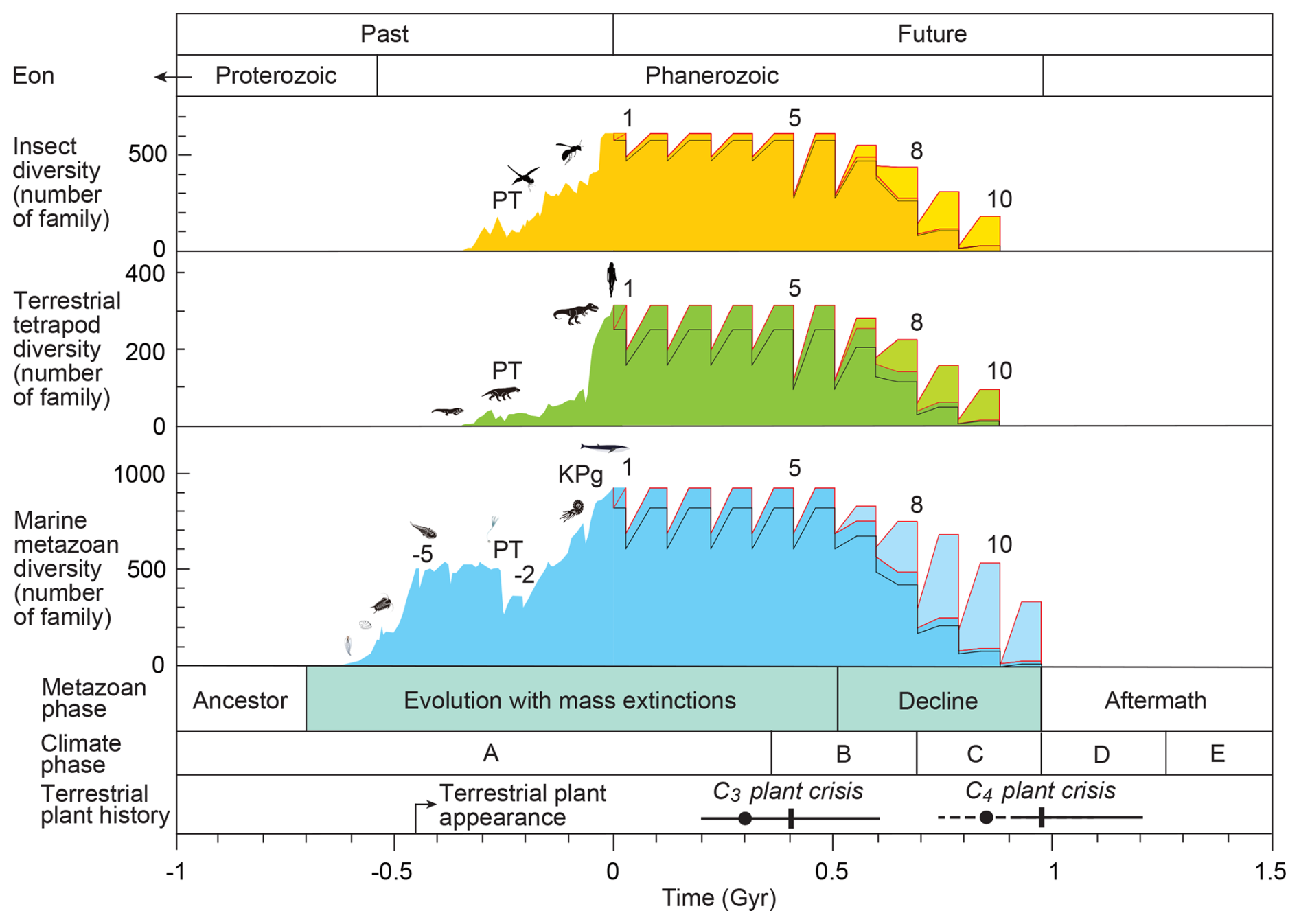
Figure 5 Changes in the diversity of insects, tetrapods, and marine metazoan families based on four environmental–ecological models over the past 1 billion years (Gyr) and projections for the next 1.5 Gyr, alongside metazoan phases, climate phases, and terrestrial plant history. Dark-colored curves show diversity changes under the Conservative Model, in which no special evolutionary adaptation occurs in response to future low-oxygen and low-CO₂ conditions (Tables 2 and S6). Pale-colored curves represent diversity changes under the New Evolutional Model, which assumes that metazoans evolve adaptive mechanisms allowing survival under low-oxygen and low-CO₂ conditions in the distant future (Tables 3 and S6). The red curves illustrate diversity changes under the Worst Anthropocene Model. The black curves represent diversity trajectories under the Continuous Worst Anthropocene Model, in which long-term anthropogenic impacts persist through the end of metazoan history (Tables 4 and S6). Diversity data for geological time are derived from fossil records reported in previous studies (Erwin et al., 1987; Labandeira and Sepkoski, 1993; Engel and Grimaldi, 2004; Benton, 2010; see Tables S3 and S4). Future projections follow survival and recovery rates listed in Tables 2–4. Terrestrial plant crises are modeled using data from Mello and Friaça (2019) (indicated by dots and dashed lines) and Ozaki and Reinhard (2021) (indicated by solid lines). Detailed procedures for future-diversity calculations are provided in the Methods section and illustrated in Fig. 1. Abbreviations: PT = Permian–Triassic boundary extinction; KPg = Cretaceous–Paleogene boundary extinction; −5, 1, 5, 8, and 9 = event numbers.

Table 5 Definitions of abbreviations used in Eqs. (9)–(22) (all values represent family-level parameters).

Table 6 Extinction and survival rates at the genus and family levels for each latitudinal range.

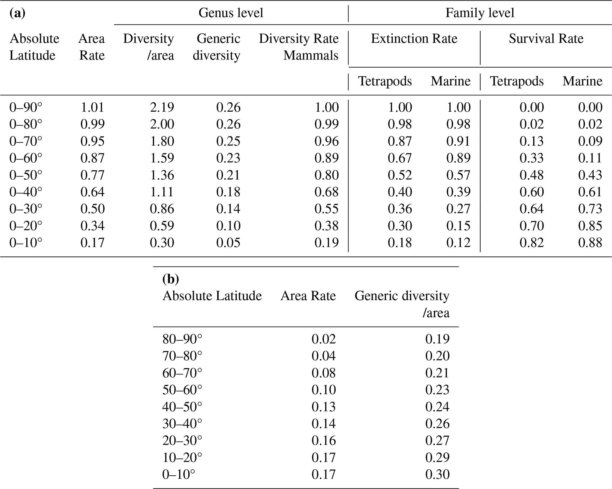
The upper portion (a) shows integrated family-level values derived from genus-level diversity (b). Genus-level diversity per km² is based on Li et al. (2021), with conversions to family-level diversity following Kaiho (2022a), Fig. 1.

Based on these results, the interval from −1.0 to +1.5 Gyr is divided into five evolutionary phases:

• (1)

  Ancestor Phase (early Climate Phase A, $<-\mathrm{0.7}$ Gyr),

• (2)

  Evolution with mass extinctions (late Phase A and early Phase B, −0.7–0.5 Gyr),

• (3)

  Decline with mass extinctions (late Phases B–C, 0.5–1.0 Gyr), and

• (4)

  Aftermath (Phases D and E, >1.5 Gyr) (Fig. 5).

During Climate Phase A, five future mass extinction events (Events 0–4) are projected, analogous to the past “Big Five” (Events −5 to −1). As in the past Phanerozoic, biodiversity is expected to recover fully after each event. Event 0 (the Anthropogenic Crisis) in the Worst Anthropocene Model reduces surviving families to 580 insects, 221 tetrapods, and 855 marine metazoans, followed by full recovery (Fig. 5 and Table S6). In the Continuous Worst Anthropocene Model, these reduced levels persist through all subsequent events, though extinction timing remains unchanged (Fig. 5, Table S6).

During Events 0–4 (0–0.40 Gyr), sharp declines are projected in the Conservative (extinction driven by low oxygen and CO₂) and New Evolutional Models (which assumes higher tolerance for low oxygen and full survival under low CO₂), reducing families from 610→494 (insects), 315→198 (tetrapods), and 950→703 (marine), based on Eqs. (9)–(15) (Fig. 5, Table S6). In the Worst Anthropocene Model, Event 0 yields 580, 221, and 855 families. Recovery is complete in all cases except the Continuous Worst Anthropocene Model, where reduced diversity persists (Fig. 5, Table S6).

Large volcanic eruptions or asteroid impacts generate severe cooling followed by abrupt warming, similar to past mass extinctions. Metazoan evolutionary phases correspond to intersections between maximum global temperatures (red dots, Fig. 2a) and GAT corresponding to the thermal survival limit of 46 °C (Local Daily Maximum Temperature [LDMT]), above which protein denaturation occurs.

From 0.4–0.7 Gyr (Climate Phase B), abrupt warming causes increasingly severe extinctions. Outside these events, diversity declines gradually due to falling O₂ and CO₂ and long-term warming associated with solar luminosity increase. By Period 9R (0.5–0.8 Gyr), insect families fall from 610→28, tetrapods from 315→14, and marine metazoans from 950→87 in the Conservative Model (Fig. 5, Table S6). Diversity falls below half its initial value at 0.65, 0.65, and 0.74 Gyr, respectively (Table S6). The New Evolutional Model yields somewhat higher diversity (Fig. 5).

At Event 10 (∼0.9 Gyr; Climate Phase C), global average temperature (GAT) reaches approximately 43 °C, reducing insect and tetrapod survival to 3 % and 2 %, respectively, in the Conservative Model (Table 2), corresponding to the crossing of the GATEL90 threshold (Fig. 2a). All superterranean taxa disappear, while subterranean taxa are able to persist only at high latitudes (60–90°; Fig. 2a). However, even these subterranean survivors – estimated at 0.01 insect families and 0.00 tetrapod families in both the Conservative and Worst Anthropocene Models, and 0.00 insect and 0.00 tetrapod families in the Continuous Worst Anthropocene Model – correspond to zero surviving species (Table S6). Therefore, both superterranean and subterranean lineages go extinct simultaneously at Event 10. The New Evolutional Model yields slightly higher values (0.06 and 0.02 families, respectively), but still results in complete extinction (Table S6).

At Event 10, approximately 0.86 and 0.77 marine metazoan families survive in the Conservative Models and Continuous Worst Anthropocene Model, respectively – translating to only a few species. In contrast, the New Evolutional Model yields 5.5 marine metazoan families (Table S6). At this stage, a few high-latitude surface-water families and a small portion of deep-water families in anoxic conditions remain in the oceans. By Event 11 (∼1.0 Gyr), marine families decline to zero in all four models. Therefore, complete marine extinction is projected to occur at ∼1.0 Gyr in the Conservative, Worst Anthropocene, and New Evolutional Models, and slightly earlier (∼0.9 Gyr) in the Continuous Worst Anthropocene Model.

3.3 Contribution factors

To evaluate the relative influence of global warming, oxygen decline, CO₂ decline, and food scarcity (FS) on the timing of metazoan extinction, I conducted a series of sensitivity experiments in which each factor was removed individually from the Conservative Model.

In the absence of abrupt global warming (i.e., removing the SRC component), the complete extinction of insects, tetrapods, and marine metazoans is delayed by approximately 0.1, 0.1, and 0.05 Gyr, respectively (Tables 7 and S8 in the Supplement). When the decline in atmospheric oxygen (RRO) is excluded, the delays are 0.1, 0, and 0 Gyr.

Table 7 Global Average Temperature for Extinction (GATE) for each habitat type (superterranean, subterranean, surface-water, deep-water) and absolute latitude. Values correspond to thresholds defined from Fig. 4 and Sect. 2.4.

Removing the CO₂ decline (RRC) results in no delay in either of two cases – whether RRC alone is held constant or both RRC and the climatic cycle are held constant (Tables 7 and S9 in the Supplement). In this scenario, long-term periodic climate oscillations are assumed to continue unchanged into the future because CO₂ does not decrease (Fig. S1). Similarly, holding the climatic cycle constant alone also produces no delay (Tables 7 and S9). Suppressing gradual warming (RRW=1) likewise yields delays of 0, 0, and 0 Gyr (Tables 7 and S10 in the Supplement). When food scarcity following the extinction of surface metazoans is excluded, the delays are 0.1, 0.1, and 0 Gyr (Tables 7 and S10). Because subterranean and deep-water metazoans inevitably experience food scarcity once surface plants and animals disappear, abrupt global warming and food scarcity function as a combined controlling factor.

Taken together, these experiments show that abrupt global warming is the dominant factor determining the timing of metazoan extinction. In contrast, oxygen decline, CO₂ decline, and gradual warming exert comparatively minor influences, primarily because their effects become substantial only after ∼1.0–1.1 Gyr (O₂ decline) and ∼1.0–1.3 Gyr (CO₂ decline). Abrupt warming begins to impose strong biological stress earlier – for example, SRC drop to 0.29 and 0.23 for insects and tetrapods at Event 9 (0.8 Gyr), and to 0.03 and 0.02 at Event 10 (0.9 Gyr) (Table 2). Thus, by ∼1.0 Gyr, oxygen and CO₂ levels have not yet become the principal extinction drivers; instead, extreme surface warming – amplified by increased solar luminosity, long-term climate cycles, and large-scale volcanism – emerges as the primary cause of terrestrial metazoan extinction.

The impact of abrupt warming on marine metazoans appears ∼0.1 Gyr later than in terrestrial groups. SRC decline to 0.09 at Event 10 (0.9 Gyr) and to 0.08 at Event 11 (1.0 Gyr) (Table 2). This lag occurs because maximum land temperatures (LDMT) exceed mean land temperatures (LMMT) by ∼3 °C, whereas maximum temperatures in surface waters are nearly identical to LMMT (Fig. 4a and c).

The half-life of diversity, occurring at 0.65–0.74 Gyr, is delayed by approximately 0.1–0.2 Gyr in simulations where O₂ or CO₂ decline is excluded, but not in simulations where abrupt warming is excluded (Table 9). This suggests that while long-term decreases in atmospheric O₂ and CO₂ gradually reduce metazoan diversity, abrupt warming is the dominant factor driving the final extinction, which occurs at 0.9–1.0 Gyr. Specifically, abrupt warming events cause sharp drops in SRC, directly leading to complete metazoan extinction.

Table 8 Recovery rates for terrestrial and marine metazoans, calculated using Eqs. (15)–(22).

Rates incorporate oxygen decline (RRO), CO₂ decline (RRC), and warming/anoxia effects (RRW, RRWA).

Table 9 Estimated ages of complete extinction and 50 % diversity loss for insects, tetrapods, and marine metazoans under four primary models and seven hypothetical test scenarios.

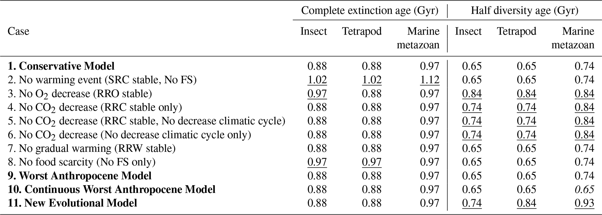
Underlined values indicate delays relative to the Conservative Model, while italicized values indicate earlier occurrences. Cases 2–10 are modified versions of the Conservative Model, among which Cases 2–8 represent hypothetical test scenarios that are not considered realistic.

4 Discussion

4.1 Characteristics of future diversity estimation in this study

A remaining biosphere lifespan of ∼1.2 Gyr has been proposed as a plausible median estimate (Jebari and Sandberg, 2022). When only the long-term warming trend driven by gradually increasing solar luminosity is considered (Mello and Friaça, 2019), metazoans go extinct at Event 14 at ∼1.3 Gyr for marine taxa and Event 13 at ∼1.2 Gyr for terrestrial taxa, based on the intersection of the black dashed line with the upper boundary of GATES90 following the logic in Sect. 3.2 (Fig. 2a). Under the oxygen-depletion scenario of Ozaki and Reinhard (2021), atmospheric O₂ falls below ∼0.01 PAL at ∼1.1 Gyr – sufficient to induce metazoan extinction. The present study indicates that metazoan demise occurs 0.1 Gyr earlier than estimates based solely on long-term warming and accompanied atmospheric O₂ and CO₂ loss, except for marine metazoans under the New Evolutional Model.

This discrepancy arises because previous models do not incorporate the effects of extreme surface-temperature anomalies linked to mass-extinction–scale events. In contrast, the estimates produced here integrate all major drivers of future temperature variability – long-term warming trends, climatic cyclicity, cooling effects tied to long-term mantle-temperature decline, gradual decreases in O₂ and CO₂, and abrupt catastrophic events – together with group-specific physiology and habitat constraints, providing a more realistic projection of conditions leading to metazoan extinction.

Extinction or survival rates during abrupt events are critical for understanding the fate of particular taxa – including humans – and for determining the final extinction timing of each metazoan group. However, these rates have less influence on long-term biodiversity trajectories. Instead, recovery rates (RR) under gradual environmental change strongly shape long-term diversity patterns (Eqs. 9 and 10).

Figure 3 shows a positive relationship between oxygen levels and biodiversity. The emergence of terrestrial metazoans likely required elevated atmospheric oxygen, because survival on land depended on the formation of an ozone layer capable of blocking harmful short-wavelength UV radiation. This dependency provides a possible explanation for why terrestrial insects and tetrapods exhibit lower recovery rates than marine metazoans after ∼0.5 Gyr (Fig. 5).

Because comprehensive fossil records for non-insect terrestrial invertebrates are lacking, Fig. 5 presents only the diversity trajectories of tetrapods and insects. Nonetheless, most terrestrial invertebrates are expected to follow similar trends, given their comparable upper thermal-tolerance limits. These organisms predominantly occupy surface environments or shallow soil layers, where thermal regimes closely match those experienced by insects and small vertebrates (Somero, 1995; Pörtner, 2002). Therefore, their future biodiversity trajectories are expected to parallel those of terrestrial insects and tetrapods.

Sea-water temperature is uniform at a given location, whereas land temperatures vary depending on sun exposure. Because land temperatures in this study correspond to shaded conditions, the results reflect extinction and survival rates based on the assumption that organisms would die even if they sought refuge in the shade. Thus, the extinction and survival rates presented here are robust.

4.2 Reliability of future biodiversity projections

Future metazoan diversity is shaped by seven primary forcings:

• (1)

  the long-term increase in solar luminosity,

• (2)

  long-term (0.35–0.30 Gyr) hothouse–icehouse climate cycles,

• (3)

  abrupt climate disruptions linked to major mass-extinction processes,

• (4)

  progressive CO₂ decline,

• (5)

  progressive atmospheric oxygen decline, and

• (6)

  the anthropogenic crisis.

Accordingly, the reliability of future biodiversity projections depends on six key considerations:

• (1)

  whether solar luminosity remains the dominant control on the persistence or extinction of life,

• (2)

  whether long-term hothouse–icehouse cycles continue to operate,

• (3)

  whether abrupt climate perturbations associated with mass-extinction-scale events continue to occur,

• (4)

  whether CO₂ decline induces major plant crises,

• (5)

  whether atmospheric oxygen decline significantly alters metazoan diversity, and

• (6)

  whether life can survive the ongoing anthropogenic crisis, which includes CO₂-driven warming, pollution, deforestation, and the risk of full-scale nuclear conflict.

4.2.1 Solar luminosity increase

The long-term rise in solar luminosity is modeled using a suite of coupled Earth-system components – including mantle convection, quasigrey radiative models, planetary albedo evolution, effective solar flux reconstructions, surface temperature models, atmospheric water-loss processes, continental-weathering feedbacks, and simplified biosphere–climate interactions. These elements, developed by Mello and Friaça (2019) and others, capture essential feedbacks among the atmosphere, hydrosphere, lithosphere, and biosphere, providing a robust basis for projecting future global temperature evolution.

4.2.2 Long-term hothouse–icehouse cycles

Long-term (0.35–0.30 Gyr) climate cycles are reconstructed from sea-surface temperature (SST) estimates based on oxygen-isotope compositions of fossil apatite and calcite, together with evidence of glacial diamictites across multiple paleolatitudes (Scotese et al., 2021). Over the past ∼1 Gyr, three complete long-term cycles have been identified, supporting the assumption that similar cycles will continue (Fig. 5). These cycles were driven primarily by plate-tectonic and mantle processes associated with supercontinent assembly and breakup (Heron, 2018; Mather et al., 2026). The expected formation of the next supercontinent, Amasia, around 0.25 Gyr (Yoshida, 2016), aligns with the projected onset of the next major icehouse interval (Fig. 2a).

Mantle temperatures are expected to remain sufficiently high to sustain large-scale convection – ∼1350 °C at present, decreasing to ∼1250 °C at 0.7 Gyr and ∼1200 °C at 1.0 Gyr (Mello and Friaça, 2019). However, progressive CO₂ depletion due to enhanced continental weathering (driven by rising solar luminosity) will reduce the amplitude of future cycles, diminishing their climatic influence during the intervals when terrestrial and marine metazoan extinctions ultimately occur.

4.2.3 Abrupt climate changes associated with mass extinction events

Abrupt climate changes linked to mass extinction events are inferred from oxygen-isotope records of apatite and calcite associated with the five major mass extinctions. Mantle-temperature projections indicate that plume-related large igneous province volcanism will remain possible, and asteroid impacts are expected to continue occurring at rates inferred from lunar and terrestrial cratering histories (Neukum, 1983; Glikson, 1999; Hartmann et al., 2007; Kaiho and Oshima, 2025). Such high-magnitude, short-duration events will therefore likely persist as sources of abrupt climatic disruption superimposed on long-term warming.

Short-term SO₂, soot, and CO₂ releases exert minimal influence on multimillion-year temperature trends because their climatic impacts typically last <0.1–1.0 Myr. Over geological timescales, natural recovery processes – such as sulfur deposition and CO₂ drawdown – dampen these perturbations. As a result, long-term warming, cyclical climate fluctuations, and abrupt catastrophic events (as represented in Eq. 1) collectively define the global temperature trajectory (Fig. 2a).

The upper thermal tolerance limit of metazoans is strongly conserved across lineages owing to protein denaturation at high temperatures (Fig. 4), enabling robust projections of future metazoan decline and extinction.

4.2.4 CO₂ decrease – plant crises

A major C₃ plant crisis is projected to begin around 0.4 Gyr, resulting in widespread loss of trees and associated terrestrial metazoans (Fig. 5; Mello and Friaça, 2019; Ozaki and Reinhard, 2021). This crisis will likely facilitate the expansion of C₄ plants, which use CO₂-concentrating mechanisms and are better adapted to hot, arid, low-CO₂ environments. The resulting ecological shift – from forests to grasslands and eventually to C₄-dominant woody vegetation – will alter recovery rates and contribute to long-term biodiversity decline (RRC in Table 8).

Because both C₃ and C₄ photosynthetic pathways are expected to persist in marine ecosystems (Reinfelder et al., 2000, 2004), the same diversity-recovery rates (RRC) are applied to marine diversity trends, which subsequently exert cascading negative effects on global metazoan biodiversity (Fig. 5).

4.2.5 Progressive oxygen depletion

A long-term decline in atmospheric oxygen will further constrain metazoan metabolism and habitat availability, especially for large or active organisms. This oxygen limitation suppresses biodiversity recovery throughout the 0.5–1.1 Gyr interval (Ozaki and Reinhard, 2021).

4.2.6 Anthropogenic crisis

The Anthropocene crisis may cause a minor mass-extinction peak in the late 21st century (Kaiho, 2022b, 2023). However, metazoans can still survive and recover if CO₂ emissions, pollution, deforestation, and nuclear-war risks are effectively mitigated.

Because the post-Anthropocene trajectory of biodiversity depends heavily on human environmental management, this study models two contrasting conditions:

• full recovery after the anthropogenic crisis (RR=1.0), and

• no recovery (RR=0.0), in which biodiversity remains suppressed even though the final extinction timing is unchanged.

4.3 Incomplete recoveries in metazoan diversity

Four major factors are projected to limit the full recovery of metazoan diversity following future mass extinction events occurring after ∼0.5 Gyr from now:

1. Anthropogenic Crisis
   Human-driven environmental pressures – including CO₂ emissions, pollution, habitat loss, and nuclear conflict risk – are expected to inhibit biodiversity recovery until these impacts subside. Under worst-case scenarios, such as full-scale nuclear war, reduced biodiversity may persist continuously until the final extinction of metazoans.

2. Plant Crisis
   The second limiting factor is the long-term decline of terrestrial plants driven by reduced atmospheric CO₂. As CO₂ levels approach the minimum threshold required for photosynthesis, global primary productivity sharply decreases. This reduction in ecosystem energy flow constrains the capacity of both terrestrial and marine systems to sustain diverse metazoan communities, preventing full biodiversity recovery after extinction events.

3. Progressive Oxygen Depletion (0.5–1.1 Gyr)
   A gradual decrease in atmospheric oxygen further limits recovery. Lower O₂ concentrations restrict aerobic metabolism and shrink habitable environments, particularly for large or metabolically active organisms. This constraint suppresses metazoan recovery potential throughout the 0.5–1.1 Gyr interval.

4. Rising Global Temperatures During Events 8–10 and Intervening Warm Periods (0.7–0.9 Gyr)
   Extreme global temperatures – reaching 44–46 °C during Events 8–10 – exceed the upper thermal tolerance of most metazoans. Even during non-event intervals, background temperatures of 36–38 °C (similar to those during the end-Permian extinction) persist, preventing diversification and ecological rebound. These elevated temperatures also promote widespread oceanic anoxia and euxinia, driving deep-sea metazoan extinction.

Together, Factors 2–4 generate sustained declines in metazoan diversity during Events 5–12 (Fig. 5). Factor 1 – the anthropogenic crisis – further inhibits recovery for as long as it continues. An interesting implication of this timeline is that the total lifespan of metazoans on Earth is therefore estimated at 1.6–1.7 billion years – approximately 12 % of Earth's projected 12-billion-year habitable lifespan. Humanity currently exists near 40 % of Earth's metazoan history and about 30 % of Earth's terrestrial metazoan history.

4.4 Uncertainties in the timing of final metazoan extinction

Earth's surface temperature is the primary factor controlling the timing of complete metazoan extinction. Consequently, uncertainties in estimating extinction timing are closely linked to uncertainties in surface temperature projections. These include components such as the long-term warming trend, climatic cycles (icehouse–greenhouse phases), and abrupt climate shifts.

The uncertainty associated with the long-term warming trend is estimated to range from −0.1 to +0.2 Gyr, based on Mello and Friaça (2019). Uncertainty from long-term climatic cycles is ±0.1 Gyr, although this influence diminishes near the time of complete extinction. The timing of abrupt warming events carries a smaller uncertainty of ±0.03 Gyr (1σ). Additionally, variations in warming anomalies can contribute an estimated ±0.1 Gyr of uncertainty.

Further variability arises from differing responses of metazoan groups to declines in atmospheric O₂ and CO₂, as reflected in the divergent extinction timings predicted by the Conservative and New Evolutional Models.

Despite these factors, variations in extinction rates from paleontological records and differences in extinction threshold values (i.e., the number of surviving families ranging from 0.1 to 1.0) have little impact on the overall lifespan of metazoans. This is because final extinction is primarily driven by abrupt global warming events – especially those triggered by large-scale volcanism – which ultimately override other extinction processes.

Thus, the total uncertainty in the timing of final metazoan extinction, as governed by Earth's surface temperature, is estimated to range from −0.1 to +0.2 Gyr.

5 Conclusions

Future metazoan diversity will be shaped by the combined impacts of gradual global warming, abrupt climate shifts triggering mass extinctions, CO₂-induced plant crises, and progressive atmospheric oxygen depletion. These factors are integrated into the biodiversity trajectory shown in Fig. 5, which reconstructs metazoan diversity over the past 1 Gyr and projects future trends up to 1.5 Gyr. All model scenarios – despite temporal uncertainties of −0.1 to +0.2 Gyr (Fig. 2 caption) – consistently predict a long-term biodiversity decline beginning between 0.5 and 0.9 Gyr from now. This culminates in the extinction of terrestrial metazoans by ∼0.9 Gyr and marine metazoans by ∼1.0 Gyr.

The maximum and minimum temperature anomaly scenarios can shift the timing of complete metazoan extinction by approximately ±0.1 Gyr, either advancing or delaying it. In contrast, variations in extinction rates based on paleontological records and differences in extinction threshold values (i.e., the number of surviving families ranging from 0.1 to 1.0) have minimal impact on the overall lifespan of metazoans.

A central finding of this study is that abrupt climatic events significantly accelerate the extinction timeline. Without such events, global average surface temperature (GAT) would reach the upper thermal tolerance of marine metazoans only around ∼1.2 Gyr from now. At that point, declining oxygen and CO₂ would become the primary extinction drivers. However, with abrupt warming events included, sudden temperature spikes lead to earlier and more rapid biodiversity collapse. Thus, while slow geochemical feedbacks gradually erode metazoan diversity, extreme global warming acts as the proximate trigger for extinction.

Over the past 500 million years – and for the next ∼400 million years – the Earth system has repeatedly recovered from mass extinction events. However, after ∼500 million years from now, progressive atmospheric oxygen and CO₂ depletion will drive an irreversible decline in biodiversity. Abrupt events do not directly cause this long-term trend but will cross critical physiological thresholds – such as the 45–47 °C on land, 40–45 °C in surface oceans, upper thermal limit for metazoans – during a future extreme warming episode, likely triggered by large-scale volcanism.

Such catastrophic events are expected to recur. After approximately 10–11 more warming events, the combined effects of long-term solar-luminosity-driven warming and episodic spikes will breach metazoan thermal limits globally, even at high latitudes. Subterranean metazoans (a small portion of biodiversity) will vanish simultaneously, while deep-sea taxa will succumb to the compounded effects of surface heat and widespread anoxia.