Hybrid machine learning data assimilation for marine biogeochemistry

Marine biogeochemistry models are critical for forecasting, as well as estimating ecosystem responses to climate change and human activities. Data assimilation (DA) improves predictions from these models by aligning them with real-world observations, but marine biogeochemistry DA faces challenges due to model complexity, non-linearity, and sparse, uncertain observations. Existing DA methods applied to marine biogeochemistry struggle to update unobserved variables effectively, while ensemble-based methods are computationally too expensive for high-complexity marine biogeochemistry models. This study demonstrates how machine learning (ML) can improve marine biogeochemistry DA by learning statistical relationships between observed and unobserved variables. We integrate ML-driven balancing schemes into a 1D prototype of a system used to forecast marine biogeochemistry in the North-West European Shelf seas. ML is applied to estimate (i) state-dependent correlations from free-run ensembles and (ii), in an “end-to-end” fashion, analysis increments from an Ensemble Kalman Filter. Our results show that ML improves updates for previously not-updated variables when compared to univariate schemes akin to those used operationally, particularly in lead times smaller than 5 d. Furthermore, ML models exhibit some potential for transferability to new locations, a crucial step toward scaling these methods to 3D operational systems. We conclude that ML offers a clear pathway to overcome current computational bottlenecks in marine biogeochemistry DA and that refining transferability, optimising training data sampling, and evaluating scalability for large-scale marine forecasting, should be future research priorities.

1 Introduction

Marine biogeochemistry (BGC) modelling is an essential tool for understanding global marine elemental cycles (e.g., for carbon and nitrogen), as well as for understanding the response of marine ecosystems to a range of human and climate pressures (Heinze and Gehlen, 2013; Ford et al., 2018; Fennel et al., 2022). These pressures include ocean acidification, marine heat waves, and nutrient pollution which can lead to a range of consequences, such as deoxygenation, toxic algal blooms and biodiversity loss (Doney et al., 2009; Smith and Schindler, 2009; Schmidtko et al., 2017; Frölicher and Laufkötter, 2018; Fennel and Testa, 2019; Gobler, 2020). Marine BGC modelling could then support management, policy and planning across a wide range of temporal scales. Marine BGC models are often constrained by the available observations through data assimilation (DA) (Ford et al., 2018; Fennel et al., 2019), providing both multi-decadal reanalyses of past ecosystem trends and variability, as well as short-term operational forecasts (on the scale up to 5–10 d). Such operational forecasts are run by marine forecasting centres in many countries, e.g., by the Copernicus Marine Service in Europe covering the global ocean and all the major European seas (Le Traon et al., 2019).

However, marine BGC DA faces multiple specific challenges (Dowd et al., 2014; Ford et al., 2018; Fennel et al., 2019), compared to assimilation of ocean physics observations in marine models. Marine BGC models are typically more complex than physical models (a pelagic model can have tens of variables and hundreds of parameters), they are highly non-linear and relatively poorly constrained (e.g., having highly uncertain parameters) when compared to ocean physics models. Furthermore, marine BGC observations are even fewer, sparser, and more uncertain than physics observations. This brings several specific challenges for marine BGC DA, one of those being the need for multivariate DA, where a large portion of the marine BGC model state variables is updated by observations of only a small fraction of the model variables. In the context of operational marine BGC forecasting, these observations are typically satellite ocean colour-derived chlorophyll (Fennel et al., 2019; Groom et al., 2019). Furthermore the assimilation of BGC-Argo observations (including chlorophyll, nitrate and oxygen) in open ocean waters has been recently implemented in state-of-the-art operational systems (Cossarini et al., 2019; Teruzzi et al., 2021). Other products are assimilated in reanalyses or research and development (R&D) versions of the operational systems, such as optical variables (Shulman et al., 2013; Ciavatta et al., 2014; Jones et al., 2016; Gregg and Rousseaux, 2017; Skákala et al., 2020) and size-class chlorophyll (Ciavatta et al., 2018, 2019; Skákala et al., 2018; Pradhan et al., 2020), as well as types of in situ data, such as chlorophyll, oxygen and nutrients from gliders (Skákala et al., 2021). For a broader range of marine BGC DA work beyond operational applications, see many other references, e.g., Simon and Bertino (2012), Shulman et al. (2013), Gehlen et al. (2015), and Simon et al. (2015).

Different DA systems are used across marine BGC forecasting centres, including variational (Ford et al., 2012; Song et al., 2016; Skákala et al., 2018; Coppini et al., 2021), Singular Evolutive Extended Kalman filter (SEEK) (Gutknecht et al., 2019; Ciliberti et al., 2021) and Ensemble Kalman Filter (EnKF) (Bertino et al., 2021) -based methods. Although ensemble methods (e.g., EnKF) are appealing for their capability to provide uncertainty quantification and cross-covariances, the more complex marine BGC models such as the European Regional Seas Ecosystem Model (ERSEM) (Butenschön et al., 2016) or the Biogeochemical Flux Model (BFM) (Cossarini et al., 2017), currently rely on variational methods as running a sufficiently large ensemble in the day-to-day operational forecasting context can be computationally expensive. Moreover, for such complex models, variational methods update only a very limited number of unobserved variables, typically using very simple balancing principles based on the simulated structure and stoichiometry of the phytoplankton community (Teruzzi et al., 2014; Skákala et al., 2018). We will call such systems with certain approximations “univariate”, and systems that update (nearly) all model state variables as a direct result of DA “multivariate”. The multivariate updates can happen in the DA step, through ensemble-informed background¹ error covariances (as in the EnKF), through balancing schemes, such as the scheme of Hemmings et al. (2008) based on nitrogen mass conservation applied to Nutrient-Phytoplankton-Zooplankton-Detritus models (Hemmings et al., 2008; Ford et al., 2012), or through the tangent-linear and adjoint models Mattern et al. (2017). However, whenever such multivariate schemes were applied to highly complex marine BGC models (in reanalyses, or R&D), the improvement of non-observed variables was typically marginal, with several variables often systematically degraded by DA (e.g., Ciavatta et al., 2016, 2018). This provides a warning on the use of incorrect assumptions in multivariate balancing schemes or in the EnKFs and the need for better DA and/or ensemble design.

The field of machine learning (ML) has developed rapidly during the past few decades, and has seemingly found function across every level of science and culture, due to the increasing size and availability of datasets and computational power, together with the continued development of algorithms and theory (Jordan and Mitchell, 2015; Sonnewald et al., 2021). Within Earth sciences, the flexibility of ML paradigms has allowed its use in a huge variety of applications (Reichstein et al., 2019), including extensive use in physical ocean modelling (van der Merwe et al., 2007; Nowack et al., 2018; Kochkov et al., 2021). However, using ML for marine BGC models is comparatively infrequent, with the most common examples found in parameter estimation (Mattern et al., 2012; Leeds et al., 2013; Mattern et al., 2014; Schartau et al., 2017). There are only relatively few applications outside this domain such as using a statistical emulator to quantify uncertainty (Mattern et al., 2013) and the prediction of hypoxia in shelf sea environments (Skákala et al., 2023).

In this work, we investigate whether ML can capture the complex, non-linear relationships among biogeochemical (BGC) variables, and how these relationships depend on the evolving state of the system (i.e., are flow-dependent). Here, flow-dependent indicates that the statistical relationships or errors between variables vary with the current flow or dynamical state, rather than being constant or solely climatological. The relationships learned by the ML model are then used within a DA scheme, or as a full substitute for it. Thus, we are not attempting to directly emulate or improve BGC models via ML, but instead use ML to improve DA, and specifically to cope with the challenging problem of propagating information from observed to unobserved variables in single-model deterministic runs that, by definition, do not have an ensemble to estimate the necessary statistics. The main goal of this approach is to introduce multivariate DA into the system, whilst benefiting from the relatively low computational cost of ML. This study falls within a stream of research aimed at building suitable hybrid ML-DA schemes (see Buizza et al., 2022; Cheng et al., 2023, and references therein), and, to our knowledge, it is the first such attempt in the context of marine BGC.

We first use ML to learn flow-dependent correlations that are needed within a DA update step. This amounts to merging DA and ML, whereby the latter is used to accomplish a task within the DA process. We demonstrate that such an ML-based multivariate DA is efficient and accurate. As long as enough suitable data are available for training, ML is able to learn and map complex non-linear functions for propagating the information from observed to unobserved portions of the system's state.

In a second configuration, instead of merging DA and ML, DA is used to generate a training dataset, from which ML learns the full DA step in an “end-to-end” emulation (Barth et al., 2020; Fablet et al., 2021). In this context, “end-to-end” refers to a ML model trained to map inputs (such as forecast states and observational information) directly to analysis increments, bypassing traditional, hand-crafted intermediate steps. As such, the ML model learns to predict the analysis increments for unobserved variables, given the surface background state and the increment for the observed variable. Recent work by Bocquet et al. (2024) has demonstrated that the entire EnKF analysis step can be learned in this data-driven, end-to-end manner.

Specifically, we intend to answer the following questions: (a) Can we make improvements to the existing univariate DA scheme by updating a limited set of additional variables in 1D water column model, with an ML model to estimate correlations or analysis increments? (b) Can these ML models be extended to effectively update all unobserved pelagic variables? (c) Is the ML model transferable to a new location after being trained on some other location?

Our work has a potentially important application within the North-West European Shelf (NWES) operational DA system to which it is tailored. Yet we will discuss its generalisation to other comparable systems, applied to spatial domains with similar type of marine BGC dynamics. Based on the transferability of the ML model, we speculate whether it is feasible to use the ML model trained in 1D on a 3D domain and propose a methodology for doing so.

The paper is structured as follows. We first give, in Sect. 2, details on the 1D physical model, the BGC model and the configuration used. Also, we establish the setups for the DA workflow, describing the reference univariate scheme (RUS), and the use of the EnKF. Then, in Sect. 3, we outline the two ML approaches explored in this work. We also give detail on the ML architecture and climatological statistics. Next, in Sect. 4, we present and discuss our results for: updating nitrate only; updating the entire set of pelagic BGC surface variables; and testing the transferability of the ML model to a new location with different BGC behaviour. In Sect. 5, we draw concluding remarks, summarise the key findings and discuss future work.

2 Model and data assimilation setups for biogeochemistry

2.1 Physical model: GOTM

The Generalised Ocean Turbulence Model (GOTM) (Bolding and Villarreal, 1999) is a 1D water column model for studying hydrodynamic and biogeochemical processes when coupled to a biogeochemical model, in marine and limnic waters. GOTM provides the necessary physical forcing for the coupled biogeochemical model, offering a balance between realism and computational cost by using real atmospheric forcing data, relaxation profiles, and coupling at full BGC complexity, while sacrificing the explicit representation of 3D processes. This makes the system ideal for this work, where we are primarily interested in the error relationships between different biogeochemical quantities (e.g., chlorophyll to nitrate), rather than the spatial error characteristics. GOTM can be used as a stand-alone model for studying dynamics of boundary layers in natural waters, having hydrodynamic applications in investigations of air-sea fluxes (Vagle et al., 2010), surface mixed-layer dynamics (Sonntag and Hense, 2011), dynamics of bottom boundary layers with or without sediment transport (Umlauf and Burchard, 2011; Falchetti et al., 2010), and estuarine and coastal dynamics (Burchard, 2009).

2.2 Biogeochemical model: ERSEM

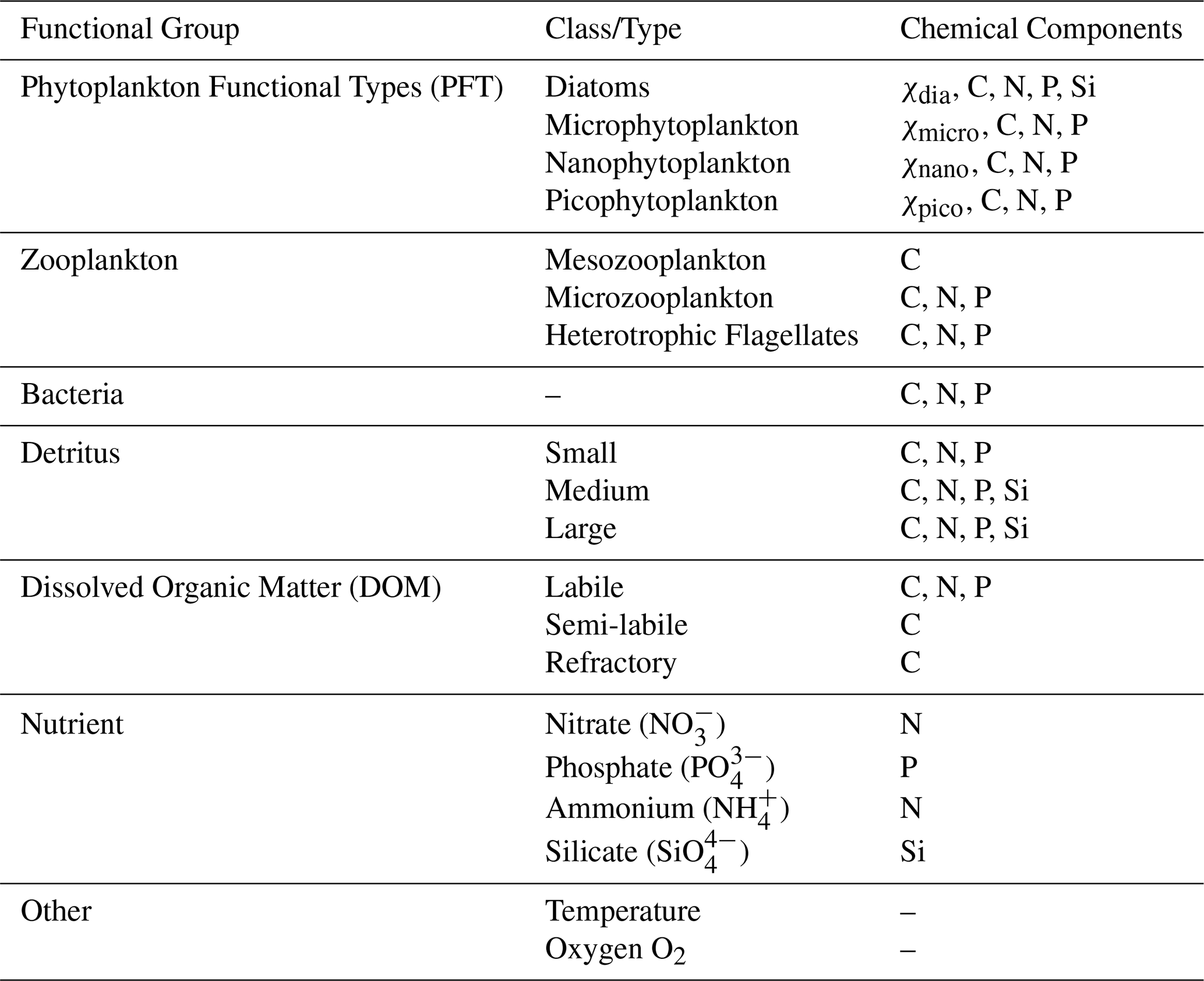
ERSEM (Baretta et al., 1995; Butenschön et al., 2016) is a marine biogeochemistry model that simulates lower trophic levels of the ocean ecosystem, including plankton and benthic fauna (Blackford, 1997), see Table 1. The model divides phytoplankton into four functional types based on size: picophytoplankton, nanophytoplankton, microphytoplankton and diatoms (Baretta et al., 1995). ERSEM uses variable stoichiometry for the simulated plankton groups (Baretta-Bekker et al., 1997; Geider et al., 1997) and represents the biomass of each functional type in terms of chlorophyll, carbon, nitrogen, and phosphorus, with diatoms also being represented by silicon. ERSEM predators consist of three types of zooplankton (mesozooplankton, microzooplankton, and heterotrophic nanoflagellates), with organic material being decomposed by a single type of heterotrophic bacteria (Butenschön et al., 2016). The model represents three different sizes of detritus (small, medium and large) and three types of dissolved organic matter (DOM: refractory; semi-labile; labile). The inorganic component of ERSEM includes nutrients such as nitrate, phosphate, silicate, ammonium, and carbon, as well as dissolved oxygen. The carbonate system is also included in the model (Artioli et al., 2012). ERSEM has been used for many applications including NWES and Mediterranean Sea biogeochemistry reanalyses (Ciavatta et al., 2016, 2018, 2019), NWES operational forecasts (Skákala et al., 2018; McEwan et al., 2021), and NWES climate projections (Wakelin et al., 2015, 2020; Galli et al., 2024).

Table 1 Reference table for ERSEM pelagic variables used in this study. Chemical components are represented by the following symbols: χ is chlorophyll; C is carbon; N is nitrogen; P is phosphorus and Si is silicon. Note that we also use total chlorophyll (denoted as chl in this work), which is a diagnostic variable calculated as the sum of chlorophyll concentrations from all PFT classes.

The coupler known as the “Framework for Aquatic Biogeochemical Models” (FABM) (Bruggeman and Bolding, 2014) allows for the smooth combination of hydrodynamic and biogeochemical models, and is used to couple GOTM with ERSEM in this work. The coupling of GOTM to marine BGC models using FABM has allowed for a wide range of applications that include modelling of phytoplankton growth (Kerimoglu et al., 2021), examining the implications of sea-ice BGC for oceanic emissions (Hayashida et al., 2017), assessing the highly intermittent spatial variability of phytoplankton on sub-grid scales (Mandal et al., 2016), and enhancing stoichiometry in existing BGC models (Anugerahanti et al., 2021).

2.3 Model configuration and synthetic data setup

We configure the GOTM-FABM-ERSEM setup for two different locations in the English Channel (see Fig. 1) and use synthetic observations of each. The first location, known as L4 (50.25° N, 4.217° W), is a highly biologically productive site with seasonally stratified dynamics (Pingree and Griffiths, 1978), influenced significantly by the outflow of the nearby Tamar and Plym rivers. Nitrate acts as the primary limiting nutrient for phytoplankton growth. It is monitored by the Western Channel Observatory (WCO) (https://www.westernchannelobservatory.org.uk/, last access: 3 September 2024) and SmartSound Plymouth (https://www.smartsoundplymouth.co.uk/, last access: 1 September 2024).

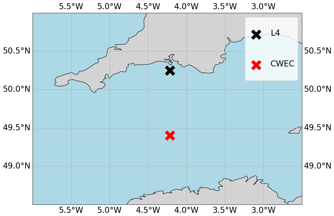
Figure 1 Map of the Western English Channel, marking the L4 model-training location with a black cross and the CWEC (Central Western English Channel) with a red cross, where we evaluated the model portability.

Besides the L4 site, we configure a setup for an additional location, that we shall refer to as the Central Western English Channel (CWEC), at 49.40° N, 4.217° W. This point is less biologically productive and it is much less influenced by riverine outflow than L4. These differences are evident when looking at the distributions of biogeochemical signals in the models applied at these two locations (see Fig. A1 in Appendix A). The differences make CWEC a reasonable alternative test site for assessing the application of the ML model, and its suitability to generalise the results of this study under different marine BGC conditions.

The physical and biogeochemical models for each location are forced with data appropriate for the study area, using the following datasets: the General Bathymetric Chart of the Oceans 2023 ($\mathrm{1}/\mathrm{240}$° resolution) for water depth; the ECMWF ERA5 dataset (0.25° h⁻¹ resolution) for meteorology; the TPXO9-atlas ($\mathrm{1}/\mathrm{30}$° resolution) for tides; and the World Ocean Atlas 2018 (0.25° resolution) for temperature, salinity and nutrient fields (nitrate, phosphate and silicate) for biogeochemical relaxation profiles. A nutrient relaxation timescale of 3 months towards the World Ocean Atlas data is required to prevent significant trends forming that cause the 1D model to gradually accumulate nutrients. This relaxation is significantly longer than the assimilation cycle of 7 d, and so has little impact on forecast errors at the surface. However, the relaxation profiles could contribute to controlling behaviour below the mixed layer in our setup (which is not updated during assimilation). This could help to mitigate some long-term biases in these areas. This is a potential limitation for operational scale systems which do not have or use these relaxation profiles.

Ensemble runs, whether as free runs or for the EnKF (see Sect. 2.4.2) are configured and run using the Ensemble and Assimilation Tool (EAT) in Python (Bruggeman et al., 2024). Each ensemble is given a spin-up period of 10 years to settle the biogeochemistry appropriately and provide well-spread initial conditions. Each ensemble member is perturbed by temporally correlated random noise to scale the ECMWF ERA wind forcing at the location. This is used to scale the wind forcing and has a correlation timescale of 7 d, a mean of 1 and a standard deviation of 0.5. The resulting variation in wind strength across the ensemble members increases their spread over time, and prevents ensemble collapse (at least within the mixed layer) induced by the previously mentioned nutrient relaxation, or lack of representation of error growth processes like horizontal advection which are absent in a 1D set-up.

For the purposes of training ML models, and generating climatological statistics, time periods for the L4 location are partitioned as follows: training data (2000–2014), validation (2015–2017), offline test (2018–2020), online test (2022–2023). Offline refers here to a setup in which the DA analysis is not then cycled as the initial condition for the next forecast, and so it does not impact successive DA cycles. Online refers to a setup in which assimilation updates are cycled, and so can have dynamical impact on later DA cycles as the model integrates in time. Climatological correlations and variances are calculated using a free-run ensemble over the training period. Because the forecasts extends seven days into the future, the number of available samples for any specific calendar day was limited, even though forecasts were issued throughout the full training period. To address this, the climatological statistics were computed as daily values, defined by averaging the statistics for a given day across all years in the training set. To increase the sample size and smooth out variability, a ±30 d window around each calendar day was applied. The CWEC location uses a run spanning 2000–2010 to generate climatological statistics, and the online test is performed for (2022–2023). No validation or offline test period is required for CWEC in this work, as we are primarily interested in a “naive transferability” of the model trained and evaluated at L4.

2.4 Data assimilation setups

We examine five data assimilation (DA) setups in this work: a simple univariate scheme representative of current operational marine BGC systems, a scheme that uses climatological statistics to update unobserved variables, an EnKF for comparison, and two novel hybrid DA schemes which are hybridised with ML techniques. Before describing each scheme, we give the basic equations of conventional DA, introduce the state vectors that the DA uses, the observation type that we assimilate, and other adjustments that are done post assimilation.

The update equation that is central to DA is sometimes called the best linear unbiased estimator (BLUE,  Asch et al., 2016; Carrassi et al., 2018) and is given by

$$\begin{array}{}\text{(1)}& {\mathit{x}}^{\mathrm{a}}={\mathit{x}}^{\mathrm{b}}+\underset{\text{analysis increment}}{\underbrace{\mathbf{K}(\mathit{y}-\mathcal{H}({\mathit{x}}^{\mathrm{b}}\left)\right),}}\end{array}$$

where K is the Kalman gain matrix

$$\begin{array}{}\text{(2)}& \mathbf{K}={\mathbf{P}}^{\mathrm{b}}{\mathbf{H}}^{\top }({\mathbf{HP}}^{\mathrm{b}}{\mathbf{H}}^{\top }+\mathbf{R}{)}^{-\mathrm{1}},\end{array}$$

x^a is the analysis (updated) state, x^b is the background state (which in this work is the state of the system after a seven-day forecast period), y are the observations, ℋ is the observation operator (with Jacobian H), P^b is the background error covariance matrix, and R is the observation error covariance matrix. The matrix P^b is of special interest to this work. Ideally this matrix should be appropriately flow-dependent, but in practice it is often not, such as in many operational schemes where a fixed climatological estimate is used. For instance, in marine BGC, we would expect the onset of a phytoplankton bloom to trigger changes in nutrient concentrations, which in turn affect the correlations between the two. This response cannot be captured by climatological statistics alone. The purpose of this work is to introduce such flow-dependency to P^b, or to the analysis increments Δx, with ML techniques. While each of the DA schemes described later will use different methods to update unobserved variables, all schemes will update total chlorophyll, the observed variable, and it's associated PFTs in the same way (using the RUS scheme described in Sect. 2.4.1).

In this work, the state vectors of the DA system, x^b and x^a, consists of the surface values of total chlorophyll and a set of chosen unobserved pelagic ERSEM variables (with chosen variable setups detailed in Sect. 3). While a state vector only considers surface values (0D), the entire DA process itself is 1D, using an idealised structure function to spread increments uniformly throughout the mixed layer. The mixed layer consists of a number of vertical GOTM grid cells, which can vary throughout the year based on the physical drivers determining mixed layer depth, such as temperature and salinity. This approach assumes that surface conditions are representative of the mixed layer as a whole (which is broadly true in this model configuration, where vertical mixing is strong enough to ensure that surface and mixed layer conditions remain well-coupled). As a result, the increments derived at the surface also provide a reasonable correction at depths/other grid cells within the mixed layer. We do not update the variables below the mixed layer, as they are decoupled or weakly coupled with the surface. Extending increments deeper would risk introducing spurious vertical structures, distorting stratification, or interfering with biogeochemical processes that are driven by different controls (e.g., remineralisation). By restricting updates to the mixed layer, the assimilation scheme ensures consistency with the available observations and avoids imposing unsupported corrections in the sub-mixed layer. Strategies for updating below the mixed layer may therefore require additional observation types (e.g., from floats or sea-gliders) or bias-correction approaches, rather than relying solely on surface observations combined with DA.

We assimilate only observations of total chlorophyll, y, at the surface. Total chlorophyll in the model, x_chl, is a diagnostic variable obtained by summing the chlorophyll content of all phytoplankton functional types (PFTs, see Table 1), which are themselves prognostic variables. In principle, one could keep only the PFT chlorophyll concentrations in the state and represent total chlorophyll via the observation operator. However, this would require explicitly summing across PFTs at every assimilation step, making the DA equations more cumbersome. Instead, we treat surface total chlorophyll directly as part of the state vector. This simplifies the presentation of the analysis equations, since the observation operator then reduces to a simple selection operator:

$$\begin{array}{}\text{(3)}& \mathbf{H}=[\mathrm{1},{\mathrm{0}}_{\mathrm{1}},\mathrm{\dots },{\mathrm{0}}_N],\end{array}$$

with the state ordered as $(x_{\mathrm{chl}},x_{\mathrm{1}},\mathrm{\dots },x_N)$. The system dimension is therefore N+1, with the first element corresponding to surface total chlorophyll, and the remaining elements corresponding to the unobserved variables to be updated. H is a row vector, as there is only one observation per DA update.

The individual PFTs themselves are excluded from the state, and instead updated after the main analysis step in Eq. (1). The surface total chlorophyll increment is redistributed across PFTs in proportion to their background contribution to total chlorophyll x_chl:

$$\begin{array}{}\text{(4)}& x_{{\mathit{\chi }}_i}^{\mathrm{a}}=x_{{\mathit{\chi }}_i}^{\mathrm{b}}+{\displaystyle \frac{x_{{\mathit{\chi }}_i}^{\mathrm{b}}}{x_{\mathrm{chl}}^{\mathrm{b}}}}\cdot \left(x_{\mathrm{chl}}^{\mathrm{a}}-x_{\mathrm{chl}}^{\mathrm{b}}\right),\end{array}$$

where χ_i stands for the chlorophyll component of each PFT, i, as in Table 1.

The associated chemical components of each PFT (C, N, P, and for diatoms also Si) are then updated in proportion to their background stoichiometric ratios with PFT chlorophyll:

$$\begin{array}{}\text{(5)}& x_{{\mathit{\zeta }}_{i,j}}^{\mathrm{a}}=x_{{\mathit{\zeta }}_{i,j}}^{\mathrm{b}}+{\displaystyle \frac{x_{{\mathit{\zeta }}_{i,j}}^{\mathrm{b}}}{x_{{\mathit{\chi }}_i}^{\mathrm{b}}}}\cdot \left(x_{{\mathit{\chi }}_i}^{\mathrm{a}}-x_{{\mathit{\chi }}_i}^{\mathrm{b}}\right),\end{array}$$

where ζ_i,j represents the non-chlorophyll components, j, of each PFT, i. This constrained redistribution scheme (Teruzzi et al., 2014; Skákala et al., 2018) ensures that phytoplankton updates preserve forecast stoichiometric ratios and remain physiologically consistent, rather than allowing a statistical method (such as the EnKF) to update PFTs freely. While we would expect an unconstrained EnKF to eventually converge towards similar balances, this explicit approach guarantees that assimilation respects acclimation dynamics and maintains the community structure of the model. Importantly, the same ratio-based balancing scheme can also be applied outside an ensemble framework in single-model runs, where it provides a consistent way of updating PFTs from a total chlorophyll correction.

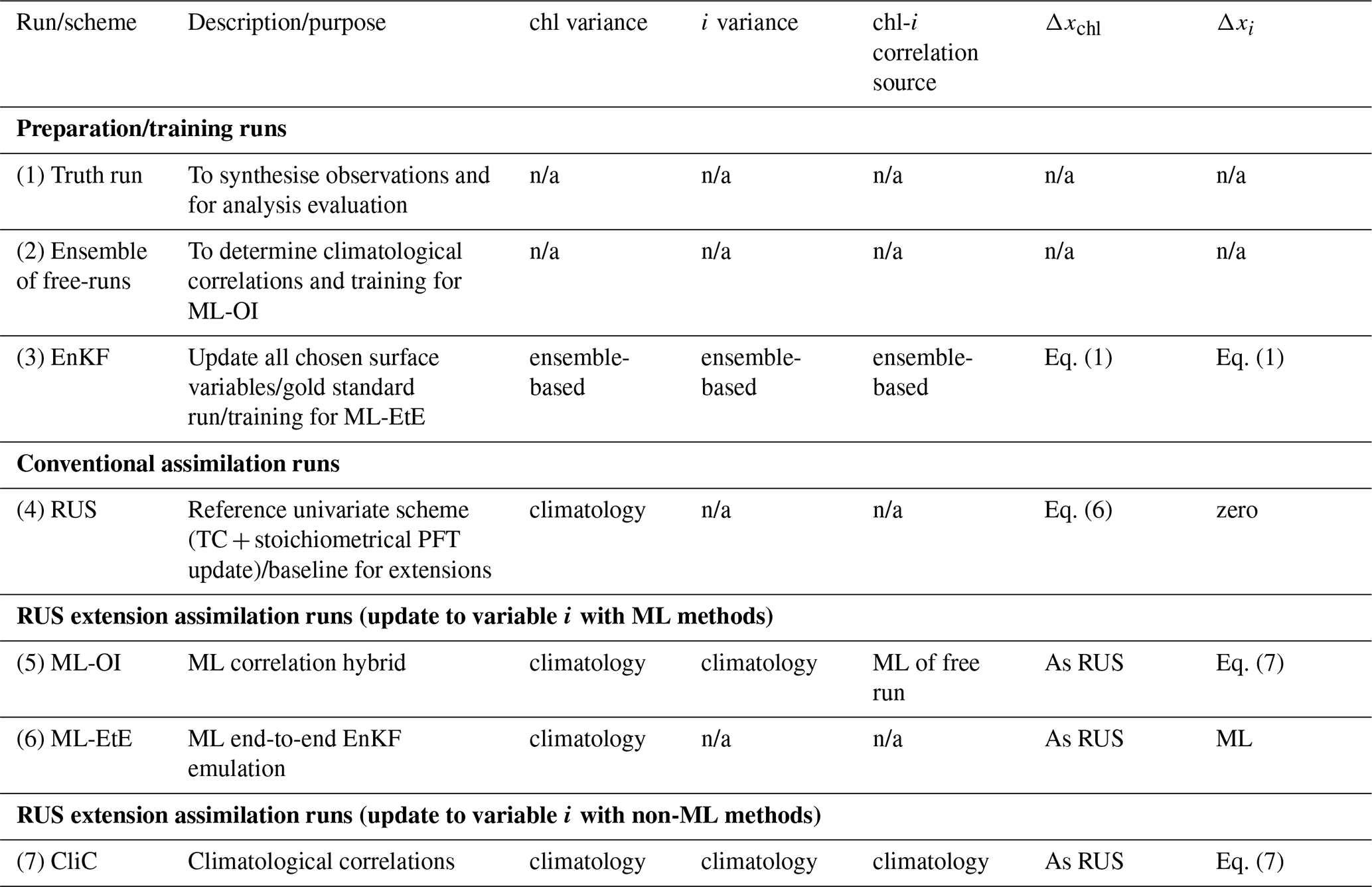
The above observation operator, and updates to the PFTs are used in all DA schemes in this paper. The specific DA schemes (conventional and ML-based) are now described. A summary of the methods is given in Table 2.

Table 2 An overview of the different run-types and schemes used in this work. Index chl refers to total chlorophyll, while index i refers to an unobserved variable (e.g., nitrate). The truth run refers to a single-model run with no updates. We sample synthetic observations from this run and feed these into each DA scheme. The ensemble of free-runs means the model is left to run without assimilation. The EnKF uses an ensemble to model background error covariance in the DA update of all state variables (Sect. 2.4.2). The RUS is the `univariate' scheme (Sect. 2.4.1), which is used as a benchmark for the performance of other schemes. It updates only the total chlorophyll state variable. The ML-OI estimates background correlations of variables beyond the total chlorophyll with an ANN (Sect. 3.1). The ML-EtE estimates the analysis increments of variables beyond the total chlorophyll produced by an EnKF using an ANN (Sect. 3.2). The CliC is similar to ML-OI but uses purely climatological background statistical estimates of the correlations to update the state of unobserved variables (Sect. 3.3). n/a stands for not applicable.

2.4.1 Reference univariate DA scheme (RUS)

We call our baseline DA method the reference “univariate” DA scheme (RUS, Table 2, row 4). Its purpose is to mimic existing DA systems used by several operational centres (Teruzzi et al., 2014; Skákala et al., 2018), although our scheme is not variational. The background error covariances are based on climatological information and so do not adapt to the state.

The RUS is based on an evaluation of Eq. (1), but only to directly update the total chlorophyll variable. The simple structure of the observation operator in Eq. (3) means we can rewrite the update Eq. (1) to show how the total chlorophyll (index chl) is updated from the total chlorophyll observation:

$$\begin{array}{}\text{(6)}& x_{\mathrm{chl}}^{\mathrm{a}}=x_{\mathrm{chl}}^{\mathrm{b}}+{\displaystyle \frac{P_{\mathrm{chl},\mathrm{chl}}^{\mathrm{b}}}{P_{\mathrm{chl},\mathrm{chl}}^{\mathrm{b}}+R}}\cdot (y-x_{\mathrm{chl}}^{\mathrm{b}}),\end{array}$$

where $P_{\mathrm{chl},\mathrm{chl}}^{\mathrm{b}}$ is the background error variance of total chlorophyll and R is the observation error variance. Climatological variances, which are used to estimate $P_{\mathrm{chl},\mathrm{chl}}^{\mathrm{b}}$, are calculated from the same period of the EnKF run (Sect. 2.4.2) used to train the ML models. Details on the training runs can be found in Sect. 3.1 and 3.2. Updates to the surface PFT chlorophyll, to the associated chemical components, and throughout the mixed layer are made separately as described previously in Sect. 2.4.

Note that we call this scheme “univariate” as only a single variable (total chlorophyll) is updated according to the background and observational errors as described in Eq. (6). All further DA schemes described in this work (apart from the EnKF below, which uses ensemble-derived covariances) start with an update of the total chlorophyll using Eq. (6), and will attempt to update additional pelagic variables using the new ML-based approaches.

2.4.2 The EnKF-based scheme

The stochastic EnKF scheme, see e.g., Evensen (2003), approximates the update Eqs. (1) and (2) with an ensemble to estimate the flow-dependent background error covariance matrix P^b, Table 2, row 3. For each ensemble member there is a different update and a different perturbed observation (the perturbations are sampled from the normal distribution 𝒩(0,R)). The EnKF updates all elements of the surface state described previously using the ensemble version of Eq. (1), but still performs the stoichiometric balancing scheme and duplication of the analysis increments from the surface throughout the mixed layer, as described in Sect. 2.4. This is done so that there is a one-to-one correspondence between the strategy used to generate the training data, and the strategy applied in the single-model schemes.

3 Hybrid machine learning data assimilation for marine biogeochemistry

In this section, we describe how we hybridise the DA, described above, with ML to provide flow-dependent estimates of the statistics/increments that are better than the climatological values. In particular, we take two approaches that differently replace parts of, or fully, the update equation. We now show the mathematical framework that the ML schemes will emulate, which is derived from Eqs. (1)–(3).

The ML-based DA schemes are summarised in Table 2, rows 5 and 6. They both build upon RUS, extending it to become multivariate. The total chlorophyll analysis is computed using the RUS update Eq. (6), while the remaining variables ($\mathrm{1}\le i\le N$) have updates according to

$$\begin{array}{}\text{(7)}& x_i^{\mathrm{a}}=x_i^{\mathrm{b}}+\underset{\text{analysis increment}}{\underbrace{{\displaystyle \frac{P_{i,\mathrm{chl}}^{\mathrm{b}}}{P_{\mathrm{chl},\mathrm{chl}}^{\mathrm{b}}+R}}\cdot (y-x_{\mathrm{chl}}^{\mathrm{b}}),}}\end{array}$$

where $P_{i,\mathrm{chl}}^{\mathrm{b}}$ is the background error covariance between variable i and total chlorophyll defined as

$$\begin{array}{}\text{(8)}& P_{i,\mathrm{chl}}^{\mathrm{b}}={\mathit{\rho }}_{i,\mathrm{chl}}\cdot {\mathit{\sigma }}_i\cdot {\mathit{\sigma }}_{\mathrm{chl}},\end{array}$$

where ρ_i,chl is their background error correlation, and σ_i and σ_chl are their respective background error standard deviations. In Eq. (7) the analysis increment of the update is labelled.

An important aspect of any DA scheme is its ability to adapt with the flow. A conventional way to introduce flow-dependency is via Monte Carlo-like methods such the EnKF, which comes with substantial computational cost. The two proposed ML-DA schemes below are designed with the above in mind and provide flow-dependency cost-effectively without the need for an ensemble (apart from at the training stage, as shall be clarified). The two ML-DA schemes are described in Sect. 3.1 and 3.2.

Regardless of the specific ML-DA scheme, each ML model is a fully connected artificial neural network (ANN) optimized using AutoKeras (Jin et al., 2019) over 100 trial configurations. AutoKeras uses Bayesian optimisation in a network search algorithm to determine optimal hyperparameters such as layer depth, layer width, dropout rate, learning rate, and optimiser selection. The input features of each model are standardised to have unit variance and a mean of zero, using data from the L4 training period during training.

Each ML approach is tested in the following scenarios: (1) a set-up where the only unobserved variable that is updated is nitrate, (2a) a set-up where we update the full set of pelagic variables, and (2b) a set-up where we update a partial set of the pelagic variables, eliminating poorly estimated variables based on the results of (2a). The progression from (1) to (2a) allows us to move from a controlled test of a single key limiting variable to a comprehensive update of the full system, while (2b) represents a refinement step that is only possible after evaluating the performance of (2a). In this way, the experimental design not only tests the limits of updating all variables, but also demonstrates how excluding problematic variables can improve robustness without discarding the broader benefits of multivariate updates. In each setup, the number of outputs to be estimated by the ML model corresponds to the number of unobserved variables. In the case of ML-OI (see Sect. 3.1), the standard deviations must also be estimated from climatology.

3.1 Hybrid machine-learning optimal interpolation (ML-OI)

This approach first updates the observed total chlorophyll and associated PFTs in an identical manner to the RUS described in Sect. 2.4.1. Then, an ANN estimates the state-dependent correlations ρ_i,chl between observed and unobserved quantities in Eq. (8) as a function of the background state (even though the EnKF update of state variables from other state variables is linear, the relationship between state variables and correlations is likely non-linear). Together with climatologically estimated values of σ_i and σ_chl (estimated using a free-run ensemble over the training period as described in Sect. 2.3), the correlations are substituted into Eq. (8) and then Eq. (7) to provide updates to the unobserved variables in the system. We call this approach ML-OI (“optimal interpolation”, Table 2, row 5). For each variable input into the ML-OI model to estimate the correlation, the background state is additionally divided by its climatological maximum at the corresponding location (before the regular standardisation procedure is applied to the data). This normalisation accounts for differences in the amplitude of seasonal variability while making an assumption that the underlying correlative relationships between variables remain consistent across locations. Since correlations are dimensionless, this scaling does not affect their interpretation, and the subsequent analysis increments (which are constructed by combining the estimated correlations with the location-specific climatological variances) remain physically consistent. Apart from correlation, the other aspect of covariance to determine are the variances. Since each variance is a single-variable statistic that can be estimated more reliably than correlations from long climatological records, we assume they are sufficiently robust to provide a stable basis for use in the Kalman gain. In contrast, correlations describe joint variability and therefore require the more sophisticated, data-driven approach described above, and cannot be approximated in the same way.

As with every approach used in this work, the resulting surface increments of the unobserved variables are then propagated to the other levels in the mixed layer, as described previously.

In order to generate training data for this approach, we run a 100-member ensemble of free-runs, configured according to Sect. 2.3 (Table 2, row 2). We generate training samples at seven day intervals across these free-runs, covering the period from 2000–2014. The features are the surface states of individual ensemble members at a given time, across all pelagic model variables. For the first application of ML-OI in Sect. 4.2, the targets are time dependent/ensemble-derived correlations between total chlorophyll and nitrate. In the later application in Sect. 4.3 onwards this is extended from just nitrate to a wider set of variables.

While the field of hybrid ML-DA is growing rapidly, there exists relatively few works in which ML-estimated background error covariances are so closely coupled with existing DA systems. However, a few particularly relevant examples stand out such as Ouala et al. (2018), in which a Kalman-like analysis update is applied to satellite-derived sea surface temperature fields using ANN-estimated background error covariances. Additional examples of this can be seen in Sacco et al. (2022), which aim to learn different sources of uncertainty using ANNs on both toy models and sea level pressure forecasts. Further work (Sacco et al., 2024) uses an EnKF to generate flow dependent background error covariances, and then learns them using a convolutional neural network.

3.2 End-to-end machine learning of EnKF updates (ML-EtE)

This approach again first updates the observed total chlorophyll and associated PFTs in an identical manner to the RUS described in Sect. 2.4.1. Nevertheless, as opposed to ML-OI, ML is used here to estimate the analysis increments for unobserved variables, given the analysis increment of the observed variable (total chlorophyll) and the complete background state. This obviously requires running a DA system to learn from. This is achieved here using the updates produced by an EnKF training run (see below). We call this approach ML-EtE (“end-to-end”, Table 2, row 6), as it emulates an existing DA system.

In ML-EtE, the analysis increment is predicted directly. By contrast, ML-OI predicts correlations, which are then combined with climatological standard deviations to form a Kalman gain, and only then applied to the innovation to yield the increment. The ML-OI scheme introduces potential sources of error – both from the uncertainty of data-driven correlation estimates and from the reliance on climatological statistics. Directly estimating the analysis increment (a vector) is also naturally more scalable for high-dimensional applications (e.g., operational 3D systems), where manipulating the full error covariance matrix (or even reduced or reformulated versions) becomes computationally costly.

To generate the training data for this approach, we first generate a nature run for the training period (Table 2, row 1), to generate synthetic surface observations of total chlorophyll concentration at weekly intervals. The observation uncertainty is equal to 10 % of the observed value. These are then assimilated into the EnKF run over the same period. The features of each training sample consist of an individual ensemble member's background state and its corresponding total chlorophyll increment from the EnKF run. The targets are the corresponding analysis increments for the unobserved variables at the surface. As described previously, the resulting surface increments of the unobserved variables are then propagated to the other levels within the mixed layer.

This approach follows other non-marine BGC work in a similar direction, such as Bonavita and Laloyaux (2020), who used ANNs to emulate the main features of an operational weak-constraint 4D-Var scheme, while Bocquet et al. (2024) pursued a similar end-to-end replacement of the analysis step. Likewise, several studies have demonstrated the emulation of analysis increments to estimate and correct model error (Brajard et al., 2020; Gregory et al., 2024). A common feature of these works is their reliance on an existing DA system or, more generally, on a robust reanalysis. The need for such a reanalysis represents a key limitation of this approach – one we revisit in the conclusion. Here, however, our primary goal is to examine the feasibility of ML-EtE and its ability to learn the EnKF updates effectively. Using this approach, the increments still ultimately come from the “analysis–background” of an EnKF, which provides a linear update to the system (even if the relationship between the state at the analysis increments is non-linear). Going beyond this limitation would require either training on increments relative to the true state (e.g., truth–background) or employing a non-linear DA system, such as a particle filter, to capture more complex, non-linear corrections.

3.3 Purely climatological updates

A further non-ML-based scheme is used to update the nitrate to mirror ML-OI, but using only climatological correlations derived from the EnKF run (CliC, Table 2, row 7) over the training period. This serves as another comparison point, a benchmark, to check whether the additional complexity of an ML model is needed.

3.4 Skill metric and machine learning model evaluation

3.4.1 Skill metric

For a system that runs for τ cycles (where a cycle represents a complete 7 d forecast and analysis), we represent the trajectory for a member i of ensemble X at cycle t as $X_{\mathrm{t}}^i$. The truth is denoted as T_t. The expected RMSE (root mean square error) over M ensemble members (or a set of M single-model runs), is calculated as:

$$\begin{array}{}\text{(9)}& \mathrm{RMSE}={\displaystyle \frac{\mathrm{1}}{M}}\sum _{i=\mathrm{1}}^M\sqrt{{\displaystyle \frac{\mathrm{1}}{\mathit{\tau }}}\sum _{t=\mathrm{1}}^{\mathit{\tau }}(X_{\mathrm{t}}^i-T_{\mathrm{t}}{)}^{\mathrm{2}}}.\end{array}$$

This is a sensible metric to use when calculating the expected error across a set of independent single-model runs, such as in the RUS, ML-OI, ML-EtE, and CliC approaches. It is also convenient for calculating the expected error of the ensemble members in the EnKF runs.

3.4.2 SHAP analysis

Shapley values are a well known and widely used metric for understanding the importance and contributions of individual input features in ML models (Lundberg and Lee, 2017). A Shapley value represents the average marginal contribution of a feature across all possible subsets of features, ensuring a fair allocation of importance. In this work, we use Kernel SHAP (SHapley Additive exPlanations) as a model-agnostic approach to estimate mean Shapely values across a dataset. Kernel SHAP approximates Shapley values by training a weighted linear model on perturbations of the input data. By calculating the mean absolute Shapley values, we measure the magnitude of influence for individual features to the model's estimations.

By understanding the importance of each input feature, we gain insight into the correlative links of dynamical behaviour in the system. This can help to identify how-and-when a model will translate well to new conditions. For example, if the primary predictive feature of an ML model is similar in two separate locations, one trained and one unseen, then we may expect the ML model to perform reasonably well in the new scenario, even if the other non-predictive features exhibit an entirely different distribution. We emphasise that we cannot infer causality from this analysis alone but understanding the data-driven feature importance and feature contribution for an ML model, combined with expert understanding of the system dynamics, can help to unveil connections and insights into the complex processes of the marine BGC model.

It also also worth noting that these metrics can also be used for feature selection with the idea that if a feature contributes little-to-nothing to the predictions, it can probably be eliminated from the feature set. This then requires the expensive processes of iteratively re-training and re-testing the neural networks and so is not an avenue that we explore in this work. SHAP is somewhat limited in the presence of highly correlated features because Shapley values assume independent feature contributions. This can lead to arbitrary or shared attributions when features provide redundant information, making it difficult to disentangle their true individual impacts. However, the correlation structures of the marine BGC have been studied previously (Higgs et al., 2024), and so can be more effectively accounted for during analysis.

4 Results and discussion

4.1 System dynamics

As discussed in Sect. 2.3, the L4 location is a highly biologically productive site with seasonally stratified dynamics. Nitrogen is a key component of organic matter and is generally the limiting nutrient to primary production by phytoplankton in coastal marine ecosystems (National Research Council and Commission on Geosciences and Water Science and Technology Board and Ocean Studies Board and Committee on the Causes and Management of Coastal Eutrophication, 2000), which includes the L4 location (Smyth et al., 2010). This leads to a strong, potentially exploitable dynamical link between phytoplankton and nitrate that varies with a clear seasonal cycle. Figure 2 demonstrates this seasonality, and how it can be broken down into three distinct regimes across any given year:

• The light-limited regime approximately spans the period from October to the start of the next spring bloom. Here, there is little-to-no phytoplankton growth due to the reduced light-levels at this time of year, meaning nutrients can be mixed throughout the water column without being used by the phytoplankton. During this period, phytoplankton concentrations are very low and mostly decoupled from nutrient dynamics².

• The bloom regime can occur throughout spring (from March until May), and is the period when phytoplankton reaches its yearly maximum. During this time, light levels no longer limit phytoplankton growth and there is a high availability of nutrients that have accumulated in the water column during the “light-limited” period. This results in a rapid increase of phytoplankton concentration, and an exhaustion of nutrients.

• The nutrient-limited regime refers to the period roughly spanning from early summer until late September where nutrients, and more specifically nitrate, have been exhausted by the phytoplankton during bloom and so concentrations are generally very low. During this time, phytoplankton relies on processes such as storms to mix nutrients into the upper water column. Consequently, phytoplankton growth is sporadic and less intense than during the spring bloom.

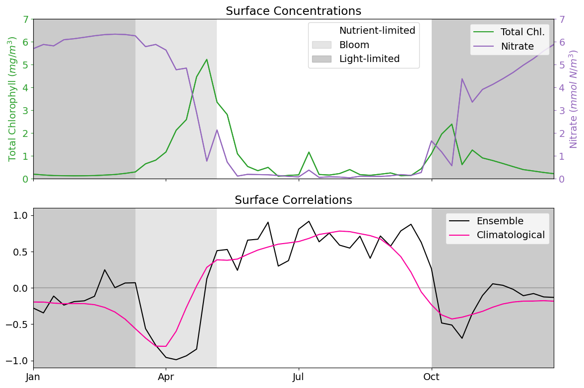
Figure 2 The top panel shows a time series for the surface concentrations of total chlorophyll (green) and nitrate (purple) during 2023 at the L4 location. The bottom panel presents correlations between total chlorophyll and nitrate derived from a 96-member ensemble (black) and from a daily varying climatology (red; calculated over the 2000–2014 training period). Shading indicates the dominant seasonal system regimes: “light-limited” (dark grey), “bloom” (light grey) and “nutrient-limited” (white).

4.2 Estimation and update to a single pelagic variable

In this section, we explore the performance of ML-OI and ML-EtE in updating only nitrate as an unobserved variable. Recall however that the observed total chlorophyll and associated PFTs are updated according to the RUS scheme in Sect. 2.4.1. We choose nitrate for these initial experiments because it is a limiting nutrient at the L4 location (see Fig. A2 and  Smyth et al., 2010), and therefore has a clear, explainable relationship with total chlorophyll as discussed in Sect. 4.1 (see also Fig. 2). Since nitrate is the key driver limiting primary production among nutrients, addressing it through DA could have a significant knock-on effect on the whole model state (through dynamical evolution from the corrected state). Moreover, this also provides the simplest proof-of-concept system to analyse initially, before we later extend the updates to more than 30 additional pelagic variables (see Table 1) in a higher complexity scenario. However, as will become clear in Sect. 4.3, this strategy for assigning importance to variables in the DA scheme does not necessarily reflect their true dynamical role in the model, highlighting the need to evaluate how different assimilation strategies and variable-update choices affect performance.

Figure 3 shows the correlation between total chlorophyll and nitrate as a function of time in the period 2018–2020 for the “offline” ML-OI experiment. The performance of ML-OI is compared to the “true correlation” computed over an ensemble of 100 members and to the correlation estimated using daily climatology.

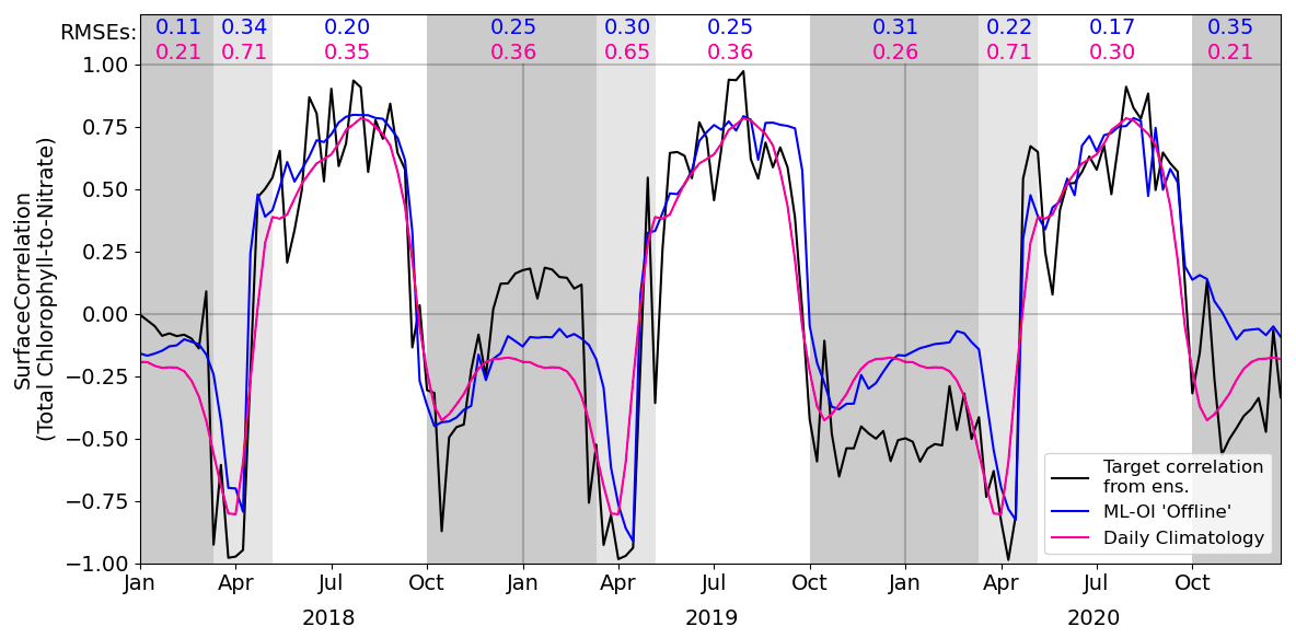
Figure 3 Estimates of correlation between total chlorophyll and nitrate, at weekly intervals across the 3-year offline test period. The target correlation (black) is calculated from the 100-member free-run ensemble (Table 2, row 2). Correlation estimates are shown for ML-OI (blue) and the daily climatology correlations (red; calculated over the 2000–2014 training period). The root mean square errors between the estimated and target correlations are given at the top of the figure, calculated separately over each regime window and for both estimation methods (with corresponding colour). The seasonal regimes of Fig. 2 are repeated.

The ML-OI model shows clear improvements over climatological estimates of correlation across most of the annual cycle. It is important to note, however, that the RMSE here only reflects the capability of a method to estimate the ensemble-derived chlorophyll-nitrate correlations. Such improvements do not necessarily translate directly to performance in an online, cycled data assimilation system (shown later) where past estimates can influence future states through the model’s dynamical evolution.

Most clearly, ML-OI is better than climatology for estimating the highly distinctive correlative pattern between total chlorophyll and nitrate during the bloom regime, showing a moderate to significant RMSE reduction in every bloom period. This pattern consists of a sharp drop to a strongly negative correlation, before an almost instantaneous increase to a strong positive correlation. These correlation patterns can be simply explained. During the bloom, phytoplankton growth exhausts nutrients, leading to negative correlations between chlorophyll and nutrients, whilst the end of the bloom, and the following period, phytoplankton growth is nutrient limited, leading to positive correlation. The precise timing of the bloom (and hence this correlation pattern) has notable inter-annual variability – varying within a period of approximately 5 weeks each year, in this model. The climatological correlations estimate this pattern poorly as they are smoothed over this period of inter-annual variability, but the ML-OI model, which estimates correlations from the state of the marine BGC model, captures the pattern much more accurately.

During the nutrient-limited regime, we see a generally strong positive correlation between total chlorophyll and nitrate, which has some local variability primarily driven by changes in wind strength, such as a weather front passing over the location and mixing nutrients into the surface. The ML-OI scheme clearly reduces the RMSE during this period, perhaps capturing some of the local variability in this “true” signal and so responds more accurately to these changes in state. Though, it is clear that the correlations of the ensemble still vary more strongly than the climatological and ML-based correlation estimates.

Finally, we also see that during the light-limited regime, the system can exist in either a “weakly positive or no correlation” state, or a “moderately negative correlation” state. However, both the climatological and ML estimates fail to capture these possible states (both predicting a weakly negative correlation over the period). During this time, total chlorophyll and nitrate are generally decoupled, and there is no clear link between the state of the system and the correlations estimated. Furthermore, as the concentrations of total chlorophyll are very near zero at this time of year (both in the ensemble and observations) and there is little spread in the ensemble – the resulting DA updates are small and have very little impact. This means that any improvement or degradation in correlation estimates at this time of year are less likely to result in any great improvement to the system, as there is weak relationship between chlorophyll and nitrate DA increments and the updates are small. However, updates at the start of this period can be important, as the resulting store of nitrate in the upper water column could have dynamical impact in later DA cycles when light is no longer limiting and the next bloom period starts.

After demonstrating the capability of the ML model to estimate the chlorophyll-nitrate relationship in an “offline” setting in Fig. 3, in Fig. 4 we compare the performance of a standard EnKF at different ensemble sizes with the schemes previously summarised in Sects. 2.4 and 3. This is done in an “online” setting, so that any update to the system can have dynamical impact on later DA cycles as the model integrates forward in time.

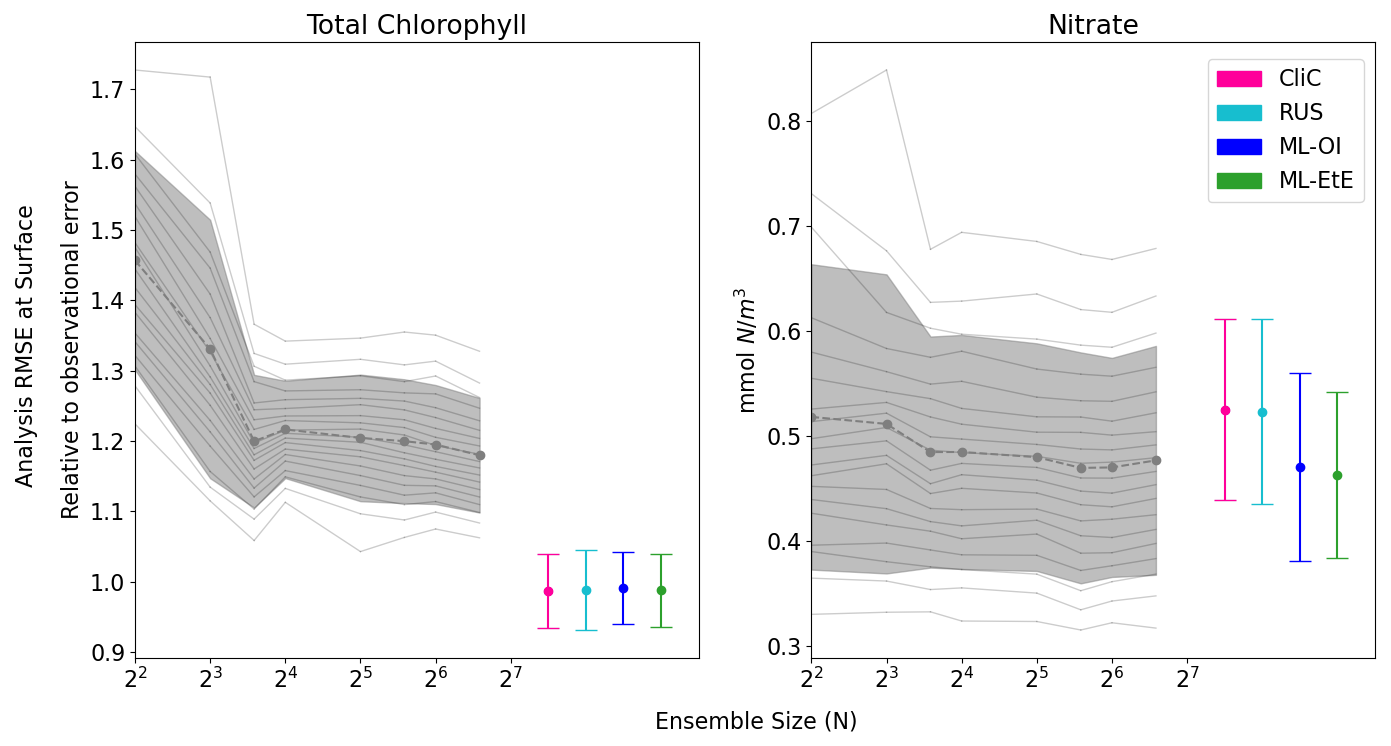
Figure 4 The relationship between analysis RMSE (Eq. 9) and ensemble size for EnKFs with different ensemble sizes, as well as the performance of the different single-model run schemes. The left panel shows the RMSE of the observed variable, total chlorophyll, normalised relative to the observational error. The right panel shows the RMSE of the unobserved variable, nitrate. The black dashed line represents the mean expected ensemble member error, from an aggregated pool of ensemble members taken from 20 repeat experiments of an EnKF at increasing ensemble sizes, with the shaded grey area indicating ±1 standard deviation of ensemble member error. The mean error and ±1 standard deviation of 64 independent single-model runs are also given for each of the methods summarised in Sects. 2.4 and 3. An extended version of the plot, showing a wider range of unobserved, not updated variables is given in Fig. B1 in Appendix B.

Figure 4 displays the performance of the EnKF, the RUS scheme, the climatological statistics scheme (CliC), and the ML schemes. Each panel shows the mean expected error of ensemble members for ensemble sizes ranging from 4 to 96. In the left panel for total chlorophyll, the relative RMSE is calculated as a ratio of the observation error. The EnKF achieves near-optimal performance for ensemble sizes greater than 16, after which the mean expected error reaches a plateau. The relative analysis error of total chlorophyll exceeds a value of 1 because it is based on the expected error of ensemble members, not the ensemble mean (see Sect. 3.4.1). This reflects the additional stochastic error introduced by the EnKF’s generation of perturbed observations. We also see, in the right panel, that the error decreases with ensemble size for the unobserved nitrate, indicating that the system converges towards more correct nitrate updates at larger ensemble sizes.

As expected, the analysis error in the observed total chlorophyll is generally comparable across each scheme because they all use the same method, the RUS scheme of Sect. 2.4.1, to update the observed total chlorophyll. However, there are more noticeable differences in the schemes that extend the updates to nitrate as well. We can clearly see that both the RUS scheme (no update to nitrate) and the CliC scheme (update of nitrate using climatological covariances in Eq. 8) perform similarly poorly for nitrate – meaning that the information provided by the observation has not propagated well to the unobserved variable. In contrast to this, both ML approaches result in a significant improvement in performance, reducing analysis error by between 8 %–12 %. This means that the information from observations can effectively propagate to the unobserved variables in a single-model run, without the need for an expensive ensemble to model the statistics at run time. ML-EtE shows similar improvements during the online testing period as those observed in the offline experiment (Fig. 3), indicating that the benefits persist even when the updates from each DA cycle feed into subsequent ones. Moreover, ML-EtE exhibits a lower standard deviation than ML-OI, indicating reduced sensitivity.

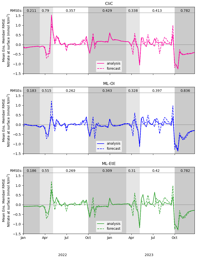
Figure 5 A comparison of mean nitrate background and analysis errors produced in the single-model runs for schemes using “online” cycled-DA at the surface. The first panel shows the analysis RMSE (solid red) and the background RMSE (dashed red) of the CliC runs. The second panel shows the analysis RMSE (solid blue) and the background RMSE (dashed blue) of the ML-OI runs. The third panel shows the analysis RMSE (solid green) and the background RMSE (dashed green) of the ML-EtE runs. For each seasonal regime, the mean analysis RMSE across the entire period and across all initialisations is given at the top of each panel. Shading indicates the system regimes previously outlined in Sect. 4.1: “light-limited” (dark grey), “bloom” (light grey) and “nutrient-limited” (white).

These single-model schemes are then investigated further in Fig. 5, looking at the analysis increments generated in the “online” setting, and their differences to the truth.

While Fig. 4 shows that they improve on average, Fig. 5 gives detail on when improvements are made. The runs shown here receive the same observations of the truth, and use the same initial conditions and forcing. However, the cycled “online” DA implies that the background state of a given time step will differ between methods. Nevertheless, we can see when ML-OI, or ML-EtE, make improvements over CliC. A clear example of this is the improved estimations during the bloom period, where the ML-estimated methods both provide a lower RMSE than the CliC. This shows that both ML methods are able to react to the timing of the bloom event much more accurately than climatology can. During the nutrient-limited period, we generally see comparable performance across the methods, as the expected correlations are generally high, and the ML-OI method can only weakly estimate the variation over this period (as seen previously in Fig. 3). ML-EtE provides no obvious advantage in this case, and explains why all methods struggle to make good increments in the second year of analyses (where the 7 d forecast errors are typically larger than in the first year). We can also see that each approach makes little to no adjustment during the majority of the light-limited regime. However, the increments by both ML-OI and ML-EtE at the start of this regime appear to yield a prolonged benefit once the system becomes inactive over winter. While these increments are unlikely to have any major impact on the system, it is interesting to note that the increments from each approach accurately reflect the expected “decoupling” of total chlorophyll to nitrate at this time of year. This corroborates with offline experiments of Fig. 3, where the ML-OI model (and indeed, the climatological estimates) struggle to replicate the correlations over winter, as there is no strong dynamical relationship between the variables at this time.

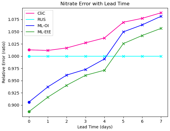
Figure 6 The forecast RMSE of each scheme relative to that of the RUS scheme at daily lead time intervals at the surface. For each scheme, the dot indicates the relative analysis error, while the crosses shows the relative forecast error for each day of lead time until a maximum lead time of 7 d – which is the total time between observations of total chlorophyll in these experiments.

Finally, Fig. 6 shows analysis and forecast errors in nitrate in each scheme where errors are normalised against the error in the RUS scheme. The daily climatological correlations scheme (CliC, red line) degrades the analysis error and then makes worse forecasts at every lead time when compared to the RUS scheme, which does not update the nitrates at all. As previously noted, both ML approaches provide an analysis state that is approximately 8 %–12 % better than the not-updated RUS nitrate. Improved forecasts then persist for approximately 4–5 d of lead time, only reaching an increased relative error after 5 d. For all lead times, ML-EtE outperforms ML-OI. While this is a net benefit to the forecasts of the system, it highlights the difficulty with partially updating a highly non-linear system. In this, it is clear that each attempt to update the nitrate results in an eventual error growth beyond simply not updating the system. Part of this could stem from the role of nitrate as a limiting nutrient; in that it is either available to allow phytoplankton growth, or not. This means that when estimating an increment for nitrate, we can know that some nitrate should be present or not, but a precise, continuous quantity that should be added or removed is not information that can necessarily be inferred from the observation of total chlorophyll. However, this error growth could also result from the analysis increments introducing some additional imbalance in other quantities of the system that also need correcting, and the complex marine BGC processes are inter-dependent. These imbalances and forecast error growths are discussed further in the following Sect. 4.3, when updating the additional marine BGC variables.

In the context of operational systems, such as those implemented by the UK Met Office, total chlorophyll is assimilated on a daily cycle, and then a forecast is produced for up to six days of lead time from these improved initial conditions. These results imply that there are huge gains to be made not only in short term forecasting (before errors saturate again), but also in reanalysis products that assimilate data with higher frequency, as the ML approaches substantially outperform the RUS scheme at this point.

4.3 Extending the set of updated variables

In this section, we demonstrate the additional benefit of estimating updates not just for nitrate, but for nearly all marine BGC variables. In Fig. 7, we compare the different ML approaches for updating an extended set of unobserved marine BGC variables, as well as the previous system that only updates nitrate.

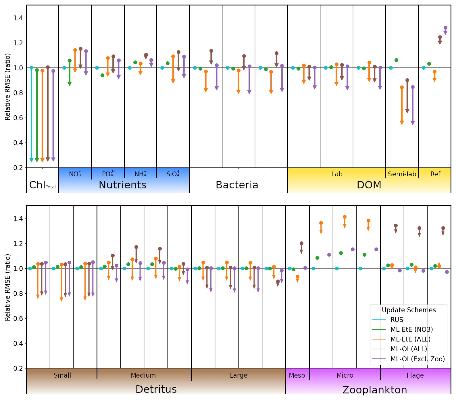
Figure 7 A comparison of the different schemes implemented to update the various components of the ERSEM BGC model at the L4 location. Surface RMSEs are calculated as an average across the entire online test period and across all initialisations. Forecast state (and equivalently background state) RMSEs at 7 d lead times are shown with dots, and the corresponding arrows indicate the analysis RMSEs (no arrow indicates the variable is not updated by the scheme). All RMSEs are relative to the RMSE in the RUS scheme shown in cyan, which only updates the total chlorophyll and PFTs as described in Sect. 2.4.1. The RMSEs of the ML-EtE (NO₃) scheme, green, are from the same experiment shown previously in Sect. 4.2, and is used as another comparison point for the extended schemes. The ML-EtE (ALL) and ML-OI (ALL), orange and brown respectively, extend the ML schemes described in Sect. 3.2 and 3.1 to update all other pelagic variables. Finally, ML-OI (Excl. Zoo) (purple) updates all pelagic variables, excluding the zooplankton types. The chemical components of each variable class/type follow the same order (left to right) as Table 1.

The RUS scheme, described in Sect. 2.4.1, is used as a benchmark for the extended schemes, and so values shown in Fig. 7 are RMSEs for 7 d forecasts relative to the RMSE of the RUS method (averaged across the 104 forecast-analysis cycles of the entire test period). Again, we recall that the RUS does not update any variables beyond total chlorophyll (shown) and its constituent PFTs (not shown). The ML-EtE (NO₃) scheme (green), which updates only nitrate, is carried over from the previous section (as it performed best), to act as another point of comparison for the extended schemes. Before discussing the extended schemes, we can see from Fig. 7 the dynamical impact that the updates of ML-EtE (NO₃) have on other (i.e. non-updated) marine BGC variables in the system. Generally, the change in RMSE for these non-updated variables is very small, with the largest improvement being to phosphate and the largest degradation to zooplankton types – particularly microzooplankton. It also slightly worsens the forecast error for ammonium and silicate concentrations that are not updated during the analysis. While this shows that updating a key nutrient, such as nitrate, can have wider impact on the system through dynamical adjustment, the generally beneficial results of the extended schemes (discussed below) point towards needing a DA system that can make reasonable adjustments to a wider set of marine BGC variables.

Our next scheme, ML-EtE (ALL) (orange), again follows the approach described in Sect. 3.2, but extends updates to all shown pelagic variables by estimating analysis increments directly from each background state and total chlorophyll increment. In this L4 setup, this is generally the best performing scheme, improving unobserved forecast and analysis RMSEs by between 10 %–50 %. We emphasise that while many of the 7 d forecast RMSEs are similar or even degraded compared with RUS, many of the benefits from an improved analysis persist over a significant portion of the forecast window (as is shown and discussed later). The most notable exceptions are the zooplankton which, despite having analysis increments in the correct direction, still return noticeably higher forecast/analysis RMSEs than most other schemes. Zooplankton have more interactions with other system components, existing at a higher trophic level, which result in a wider range of uncertainty for their behaviour. This also suggests they have generally weaker correlations with total chlorophyll. In our configuration, the RMSEs of the zooplankton group are clearly highly sensitive to updates in other variables, whether only nitrate is assimilated or a broader set is considered. When correlations between total chlorophyll and zooplankton are weak (as seen in Fig. A2), chlorophyll increments contribute little information for correcting the zooplankton field, which is already strongly influenced by changes elsewhere in the system.

The ML-OI (ALL) scheme (brown) described in Sect. 3.1, extends updates to all shown pelagic variables by estimating the inter-variable correlation from the background state only. This estimation is then combined with daily varying climatological variances to update the marine BGC state. This method is also shown to be somewhat effective, generally providing similar behaviour to the ML-EtE (ALL) scheme, or at least reducing the RMSE from forecast to analysis (even if it is still worse that the RUS in some cases). It does suffer from the same difficulty in estimating zooplankton updates, to an even greater degree, which causes some further imbalance in the system. This becomes clear when we exclude the zooplankton types from the updating in the ML-OI (Excl. Zoo) approach (purple), since it generally equals or makes small improvements over the ML-EtE (ALL) and ML-OI (ALL) schemes.

Figure A2 shows that correlations between surface total chlorophyll and silicate (or phosphate) are as strong as those with nitrate. This suggests that updates of similar magnitude might be expected for the other nutrients as well. However, it is not straightforward to infer how the system would evolve when all nutrients are updated simultaneously, based solely on the behaviour observed when only nitrate is updated. For example, Fig. 7 reveals clear differences in the forecast and analysis RMSE for nitrate between the two ML-EtE configurations: one updating only nitrate and the other updating all nutrients. In the case for ML-EtE (ALL), updating all nutrients degrades the nitrate RMSE in the forecast and provides negligible impact on the analysis, while improving the analysis RMSEs for phosphate, ammonium and silicate. This outcome is notable, as it may point to assimilation biases introduced by the choice of update strategy.

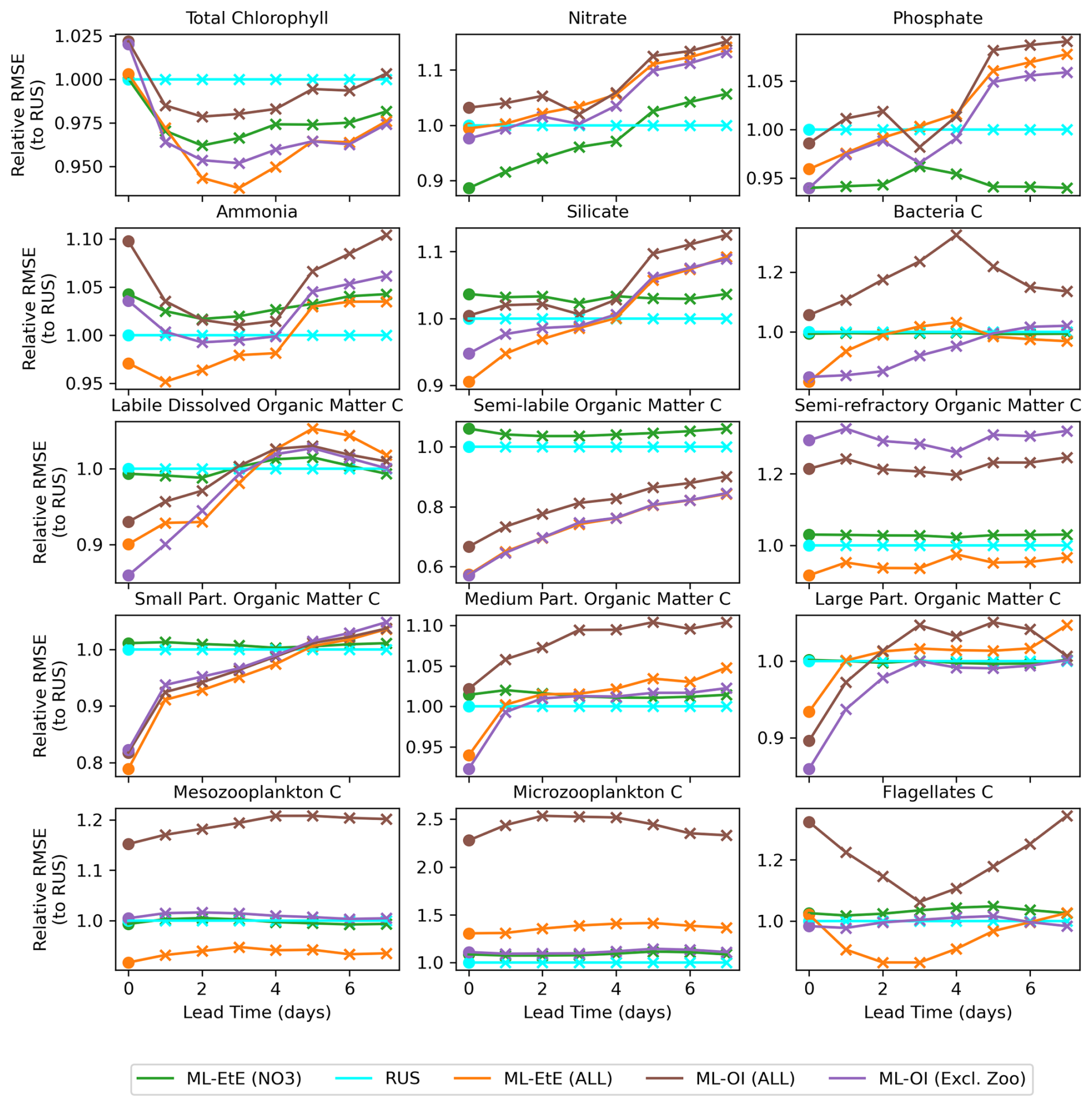
Figure 8 A comparison of the different schemes implemented to update the various components of the ERSEM BGC model at the L4 location (colours used are identical to Fig. 7). The forecast RMSE of each scheme are relative to that of the RUS scheme at daily lead time intervals. The dots indicate the relative analysis error, while the crosses show the relative forecast error for each day of lead time until a maximum lead time of 7 d, which is the time between observations of total chlorophyll.

Figure 8 shows the mean RMSE at multiple forecast lead times, for each method relative to the RUS scheme. A variety of variables have been selected from Fig. 7 to represent the different behaviours observed across each variable group. For many variables, there are notable improvements made over the first 3–5 forecast lead times (e.g., most schemes for phosphate, ML-EtE (ALL) and ML-OI (Excl. Zoo) in silicate, and the particulate organic matter variables), even if the gains do not persist for the entire forecast window of 7 d. It is also important to note that the rate at which gains are lost is not necessarily quasi-linear for some variables. For example, small particulate organic matter loses around half of its 20 % gain from the analysis time to 1 d forecast time. Interestingly, the total chlorophyll shows similar error relative to the RUS scheme for each other scheme at the analysis time (they all handle the observations in the same way, so this should be expected), but each scheme then makes improvements at essentially every other forecast lead time. This is likely due to the dynamical adjustment of the model (where gains have been made in other variables) propagating through to the total chlorophyll values as the model evolves. It is through this dynamical complexity, however, that we see other variables do not improve or degrade monotonically as lead time increases (e.g., bacteria and flagellates).

In summary the experiments from Figs. 7 and 8 show that the impact of DA analysis updates on the model forecast is not straightforward due to the non-linear and complex nature of the BGC model. Although in general it is true that increasing the number of updated variables benefits the forecasts, especially at shorter lead times (e.g., less than 5 d), this is definitely not true for every variable. Some variables, for instance, show similar or worse forecast RMSE at a 7 d lead time than the RUS, which highlights the need to evaluate how different assimilation strategies and variable-update choices affect performance.

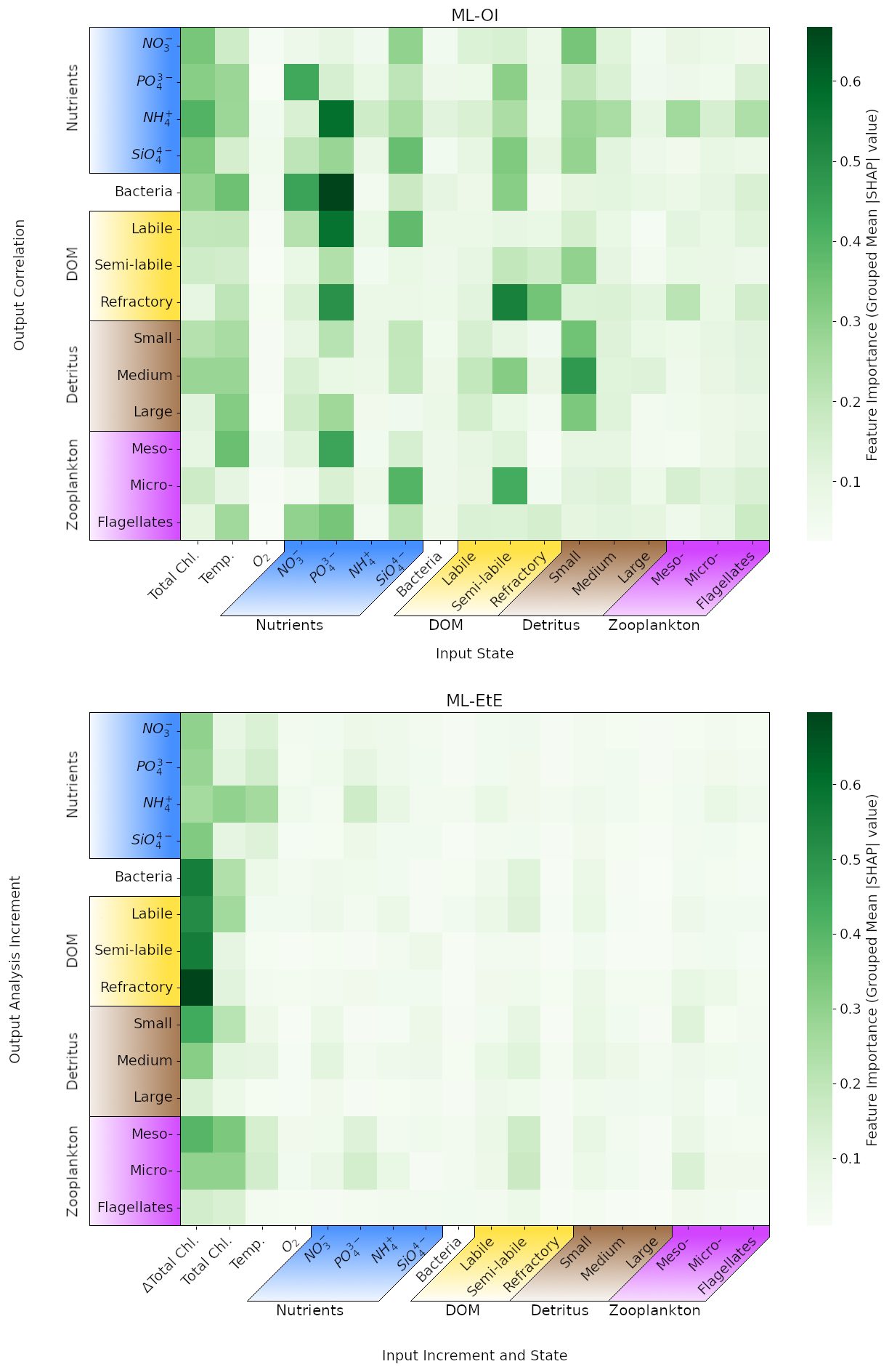
Figure 9 Mean absolute Shapley values estimated for the ML-OI (ALL) and ML-EtE (ALL), across their respective training datasets (see Sect. 3). Chemical components that belong to the same class or type (e.g., the carbon, nitrogen and phosphorus of bacteria) have been grouped as they are highly correlated. The variable names and chemical components are detailed in Table 1. The upper panel shows values for the extended ML-OI (ALL) model, and the lower panel for the extended ML-EtE (ALL) model. The grouped input features for each ML model are given on the x-axis, which make up the surface state for each pelagic variable. ML-EtE (ALL) has one additional feature, ΔTotal Chl., which represents the total chlorophyll analysis increment. The grouped output targets for each ML model are given on the y-axis, which correspond to the correlations between total chlorophyll and each unobserved variable for ML-OI (ALL), and the analysis increments for ML-ETE (ALL).

In Fig. 9, we interrogate the ML models using Shapley values (Sect. 3.4.2) to identify important ML-model features that are key to making accurate estimations, and drive the connections between observed total chlorophyll and unobserved variables. Such a Shapley analysis also has the potential to help reduce the number of features needed for training future models (though this was not the aim of our experiments).

Figure 9 shows the grouped mean absolute Shapley values for both the extended ML-OI (upper panel) and ML-EtE (lower panel) approaches. These are grouped as the separate chemical components of any class/type, and the resulting Shapley values, are very highly correlated. It is important to note that Shapley values differ from a pure correlation between the input and output variables. This is because they capture both direct and interaction effects, account for non-linear relationships, and can explain a model's decision-making rather than just measuring statistical association.

The ML-OI (ALL) Shapely values indicate that a broad range of input variables are important to the estimation of total chlorophyll correlations with unobserved variables, and highlight the general complexity of these interactions. We see that the state of temperature and total chlorophyll are moderately important across a broad set of variable groups. This makes sense as this ML model is estimating the correlation of a given variable with total chlorophyll, which is generally dependent on the state of total chlorophyll. However, this also implies that the seasonal regimes play a significant role in the estimations, as temperature is a clear identifier for the current time in the seasonal cycle. We note that the seasonal signal of other variables could also be important for the estimation of correlations as, in some cases, we see that at least one of the state variables in a group can be important to estimating the correlation between total chlorophyll and a state variable of the same group. For example, the state of small detritus is highly important to the entire group of detritus correlations, the states of some nutrients are generally important to the estimation of nutrients, and the semi-labile DOM is somewhat important to the wider DOM correlations. Each of the nutrients show moderate to strong importance across a wide variety of outputs, with the strongest being phosphates. The elevated Shapley importance of phosphate likely reflects interdependencies among nutrient variables, particularly given their correlated seasonal behaviour, highlighting a limitation of the Shapley framework when applied to features with shared temporal dynamics. Some input features show no strong importance to any output targets. In particular, the zooplankton types seem largely unimportant in estimation their own correlation with total chlorophyll and the variables with a stronger signal have no obvious direct relationship. This may partially explain why zooplankton performs poorly when they are updated by the ML-DA schemes, as seen previously in Fig. 7, and points towards the difficulty and uncertainty associated with zooplankton in marine BGC modelling. This is further evidenced as the zooplankton types are unimportant as input features for all other correlation estimations as well. We also see that oxygen is largely unimportant to the estimation of the correlations. This observation is consistent with the known weak impact of oxygen assimilation in ERSEM on other modelled variables (Skákala et al., 2021). This would imply that both zooplankton and oxygen could be removed from the input feature set with little impact on the overall model performance.

The ML-EtE (ALL) Shapley values take on a distinctly different structure to those of the ML-OI (ALL). Recall that ML-EtE (ALL) has a different target than ML-OI (ALL), as it emulates analysis increments directly. It also has an additional input feature, the analysis increment of total chlorophyll, which is readily available in both the training dataset and at run-time. The most striking difference is that the total chlorophyll analysis increment dominates the estimation importances, showing the highest mean absolute value in almost all estimations. This is to be expected, as the total chlorophyll increment contains information about the observation, observational error and background model covariance, which are all necessary components of the unobserved analysis increment as described in Eq. (1). This makes sense considering the seasonal variation of the model and that total chlorophyll represents this variation quite reliably according to the regimes discussed in Sect. 4.1. The state variable input features show much less importance in ML-EtE (ALL) than in ML-OI (ALL), but they are sometimes still non-zero. These non-zero values seem to correlate somewhat with the most important input features seen in the ML-OI (ALL) approach, even if they are significantly reduced overall, suggesting that the state still contributes to the inherent flow dependencies of the analysis increments.

Given the dominant role of the total chlorophyll analysis increment in ML-EtE (ALL), it is important to note that the influence of observations could differ when using real observations rather than synthetic ones, owing to potential differences in error characteristics, representativeness, or systematic biases. We would still expect the analysis increment of the observed variable to exhibit comparable importance if trained on increments derived from real observations, as demonstrated in this experiment. However, because of the strong influence of total chlorophyll increments, the overall structure and nature of the resulting updates may change, reflecting the impact of more complex and realistic observational error structures.

4.4 Generalisation of machine learned-correlations to an unseen location

In this section, we test the performance of the extended ML approaches from Sect. 4.3 trained for L4, but applied to the CWEC location (see Sect. 2.3 and Fig. 1), which exhibits different marine BGC behaviour than the L4 training location. In Fig. 10, we assess the performance of these ML models according to their 7 d forecast and analysis RMSEs. We then compare some general differences between the climatology of the two locations in Fig. 11, and then, with reference to the Shapley values shown previously in Fig. 9, we shall discern why the ML model might struggle extrapolating to the new location.

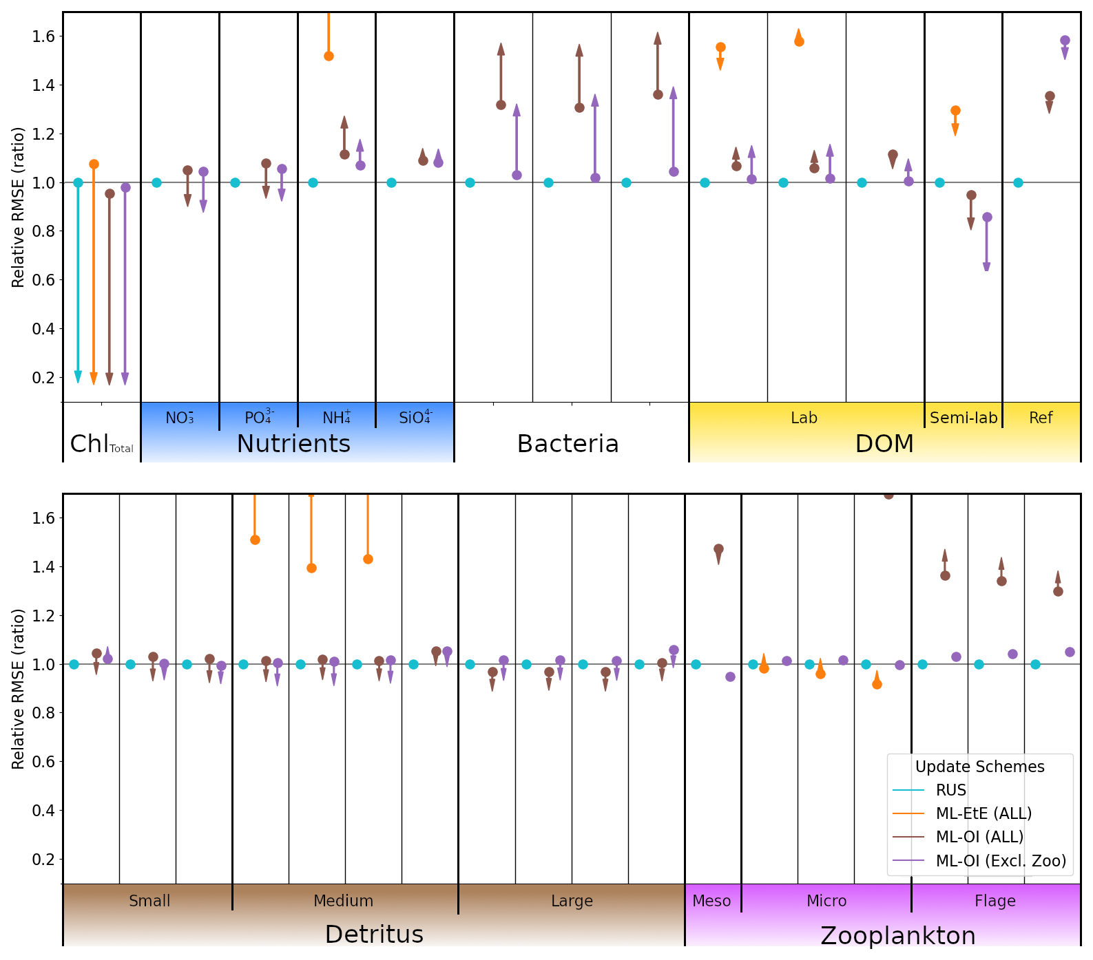
Figure 10 As Fig. 7, with the ML methods trained on L4, but applied to the new location CWEC. Dots and arrows that do not appear are off the scale.

Figure 10 again uses the RUS scheme as a comparison point for the ML model approaches, so all RMSEs are given as a ratio of the RUS's RMSE value at the new location. The ML-EtE (ALL) approach (orange) performs extremely poorly in this new location, with a large portion of the RMSEs exceeding 1.5× the RUS background error (off the scale of Fig. 10). This is because the emulated analysis increments of the EnKF at the L4 location fit the variability and scale of that (trained) location and so, do not translate well to the new location. This means that, while the ML-EtE (ALL) approach works well at the trained location (and fits the expected distribution of input data), in practice its extendability to a new location is limited by both availability of training data and to the new location's similarity to the original training location. The ML-OI (ALL) (brown) makes a marked improvement over the ML-EtE (ALL) scheme, which is the reverse of the previous scenario at the L4 location. This is likely because the correlations estimated by the ML-OI scheme represent a more location-agnostic relationship in the marine BGC variables, which can be used in combination with the climatological variances of CWEC to produce more location-appropriate increments (though this is not true for ammonium, bacteria and labile DOM, which produce a worse analysis than forecast). Furthermore, this scheme still struggles to estimate zooplankton correlations, and so not updating the zooplankton as in the ML-OI (Excl. Zoo) scheme (purple) reduces the damage compared to ML-OI (ALL) – with any improvements being marginal at best. In both ML-OI (ALL) and ML-OI (Excl. Zoo), we see that the analysis for detritus is generally improved relative to the RUS scheme (though these improvements are marginal, and of similar magnitude to the worsened forecasts). Figure 11 shows that the climatological correlations for these variables are generally similar in both locations (compare Fig. A2 and Fig. A3 to see how these vary with time), with small detritus (originating largely from species with size <20 µm) showing similarity in both climatological correlation and standard deviation. Since small detritus is the most important input feature, in Fig. 9, for the estimation of detritus correlations in the ML-OI models, it is reasonable to see why the improvements persist between the two locations. We also see in Fig. 10 that both ML-OI models (brown and purple) make improvements to the analysis RMSEs of nitrate, phosphorus and semi-labile DOM, which show relatively similar climatological behaviour to L4 in Figs. 11 and A1.

As all training is performed at one location, it is easy to hypothesise that the ML models are over-specialised to the characteristics of L4, specifically with regards to their use at other locations. Here, L4 is coastal and the CWEC is in a more open area of ocean. This does not rule out the possibility that ML models trained on a limited number of locations could extend their estimations to spatial locations beyond their set of training locations. However, it indicates that sparse training locations would need to be chosen carefully, to appropriately cover the spread of behaviour in the system.

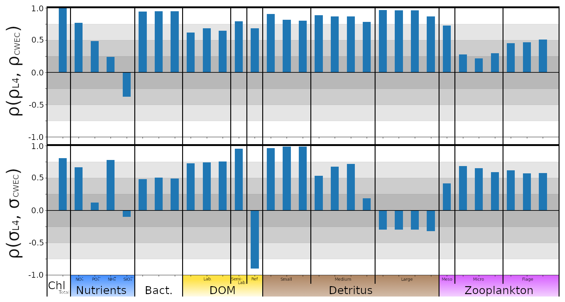
Figure 11 The top panel shows ρ(ρ_L4,ρ_CWEC), the correlation between the daily climatological correlations of each variable with total chlorophyll at L4 and at the CWEC. The bottom panel shows the correlation between a given variable's climatological standard deviation signal at L4 and the CWEC, ρ(σ_L4,σ_CWEC). High correlations indicate that the model is behaving similarly in each location.

4.5 Viewpoint on scaling multivariate data assimilation to 3D models

We have shown that ML methods can make improvements to the DA schemes of marine BGC models when coupled to a 1D physical model – particularly shown in improved forecasts for shorter lead times (< 4 d) at the training location. The natural next question is how these results would scale when the marine BGC model is coupled to a 3D physical model, such as NEMO (Nucleus for European Modelling of the Ocean). A seemingly simple solution would be to run (once) a well-tuned, large EnKF, which can then be used to train an ML model to be used operationally in an analogous 3D DA system that presently updates only total chlorophyll. A reanalysis product with comprehensive statistics, or all ensemble members available so statistics can be generated, would be ideal (Bonavita and Laloyaux, 2020; Brajard et al., 2021; Gregory et al., 2024). This circumvents the need to run an expensive DA scheme operationally as the ML model could be trained offline, and then run significantly faster while retaining the benefit of the statistics learned from a large ensemble. This would also allow the analysis increments to be estimated directly. However, state-of-the-art ensemble marine BGC systems are still limited in scale and may not (yet) accurately represent the statistics needed for multivariate DA (Skákala et al., 2024). Also, this approach would need to be repeated if/when the observation network changes, which is likely given new observation missions and strategies (Telszewski et al., 2018). A cheaper alternative would be to calculate the correlations in a free-run ensemble dataset, as per the methods described in Sect. 3.1. This would be cheaper to create as there would be no need to store and calculate both background and analysis states. However, this approach cannot calculate the analysis increments directly and instead must rely on the hybridisation of background covariances/correlations into existing DA frameworks. Nevertheless our results on the 1D scenario suggests that this is feasible and a good alternative to estimating the increments directly.

It is also worth considering how the data for these ML models should be sampled spatially in the 3D case. In this, we suggest that a sparse forest of 1D models could be generated across the 3D domain, which aims to cover each region of sufficiently different biogeochemical behaviour. Previous work by Higgs et al. (2024) has split the North-West European Shelf into dynamically connected ecoregions, and this, or similar analysis, could be used as a guideline for generating these 1D models. Furthermore, ML models could handle local multivariate aspects (a 0D transformation), while traditional DA methods (such as spatial correlations functions) manage 3D reconstruction (just as they manage the 1D reconstruction in our setup). A limitation of our two test locations is that they are not directly coupled, and could only be considered weakly coupled in the sense that their forcing data is extracted from the same 3D weather model. This could mean that 3D models have an advantage in locations having similar behaviour, as model grid points are much more likely to strongly correlate due to advection and ocean currents. However, the inverse could also be true, as the 1D models do not consider riverine input which can have substantial effects at the coast. Either way, the results suggest that some sparsity could be applied in extracting training data for these models, as long as each regime of BGC behaviour is represented in the selection. Introducing spatial variables like longitude and latitude could also improve the models ability to estimate increments or correlations across the different horizontal locations.

An additional avenue worth exploring is whether training ML models on data from multiple, sufficiently different locations could improve their generalisability. Such an approach would allow for testing whether a more generalised model can (i) perform as well as a specialised model at its training locations, and (ii) transfer more successfully to new, unseen locations. While this is beyond the scope of the present study, it represents an interesting line of future work, particularly when combined with transfer learning strategies. For instance, a model trained at one location could be used as pre-conditioning for training at a new site, with the expectation that the pre-conditioned model would require less additional data to adapt effectively (e.g., Hu et al., 2016). Together, these directions highlight the importance of balancing specialisation and generalisation when scaling ML-assisted DA from idealized 1D configurations to realistic 3D systems.

5 Conclusions

Marine biogeochemistry (BGC) models aim to represent the complex BGC processes necessary to understand and forecast ecosystem behaviour. Data assimilation (DA) plays a crucial role in ensuring model trajectories remain closely aligned with real-world observations, along with the need for continuous improvement of numerical estimations. In this study, we used a synthetic “perfect model” setup as a first step to explore ML-assisted DA under controlled conditions, but a natural direction for future work is to apply these approaches to real observations to assess their practical value. The ML-based methods considered in this study extend a conventional univariate DA system (RUS, see Table 2), which observes only total chlorophyll. One ML method (ML-OI) estimates the flow-dependent background error correlations between total chlorophyll and other model variables (which are then used in an otherwise conventional DA update step). The other ML method (ML-EtE) directly estimates the analysis increments of other model variables (bypassing the conventional DA update equations for these variables).

Both numerical modelling and DA are computationally expensive for marine BGC (dealing with great complexity and many variables), requiring well-tuned and accurately sampled statistics to be effective. These statistics are often poorly estimated in the undersized ensemble-based methods that are affordable operationally. In turn, this leads to the use of climatological background error covariance matrices in deterministic models, or simply not updating unobserved variables. This section concludes our work in relation to the research questions set out towards the end of Sect. 1 (reproduced below in italics).

(a) Can we make improvements to the existing univariate scheme by updating a limited set of additional variables with an ML model to estimate correlations or analysis increments? In this study, we have demonstrated that neural networks can effectively learn statistical relationships between total chlorophyll (the only observed variable) and various pelagic BGC model variables. With machine learning (ML), we achieve improvements over climatological statistics in the nitrate-only update framework. Our analysis of ML-estimated nitrate updates illustrates that the ML methods behave in a largely coherent and meaningful manner. While ML can degrade forecast skill in some unobserved variables compared to RUS or nitrate-only ML schemes, they nonetheless show promise, with their usefulness in more complex assimilation settings requiring further assessment.

(b) Can these ML models be extended to effectively update all unobserved pelagic variables? ML models can update almost all unobserved pelagic variables, supporting the broader applicability of ML in DA. In our configuration, zooplankton does not update well using either of the ML methods extended to all state variables (ML-OI (ALL) and ML-EtE (ALL)), and is better treated in hybrid DA schemes without being updated directly (as in ML-OI (Excl. Zoo)). This limitation may reflect the particular parameterisations of zooplankton–phytoplankton interactions, grazing, and mortality in the underlying BGC model, and may not generalise to other model setups. More broadly, we expect that variables less directly linked to or less sensitive to the observed quantity will be more difficult to update well. Since parameterisation choices can alter these relationships, new parameterisations would likely require retraining emulators, or alternatively, more flexible ML strategies such as transfer learning. Exploring such approaches in more diverse configurations remains an important avenue for follow-on investigations.

(c) Is the ML model transferable to a new location after being trained on some other location? While a neural network trained in one water column exhibits partial transferability to other locations, challenges remain in fully generalising the model across spatial domains. This partial transferability is valuable, given the difficulty and cost of acquiring high-quality training data across large oceanic regions, and should be explored further in the context of 3D models. We discuss the feasibility of this, and propose a methodology for doing so. Future work should focus on refining transferability strategies, effective sampling strategy to allow for ergodic coverage (i.e., ensuring statistical representativeness over space and/or time), and further evaluating the scalability of ML-driven DA in complex marine environments.

Appendix A: Characterisation of location biogeochemistry

Figure A1 shows the variability of each ERSEM variable over the online testing period for the L4 and CWEC locations. It shows that the CWEC is clearly less biologically productive than L4 with surface concentrations of total chlorophyll having a significantly lower median value, and a maximum that is approximately 50 % of L4's maximum. Each exhibits similar temperature values, as they are both located within the English Channel. In the nutrients group, nitrate and phosphate values cover a similar range in each location, but ammonium and silicate have little overlap. Bacteria and DOM concentrations also show little similarity between locations. The small detritus concentrations are very similar between both locations, but the medium and large detritus differ significantly, with CWEC covering a much wider range of values than L4. Zooplankton concentrations also differ between the locations, with CWEC producing much lower concentrations of zooplankton than the more biologically active L4 location.

The climatological correlations between total chlorophyll and other pelagic variables at the L4 location, shown in Fig. A2, vary significantly according to the season. Variables of the same class (see Table 1) generally exhibit very similar correlations. Correlations are much stronger during the spring and summer months, as this period is more biologically active, and so the different model components are going to be more closely coupled. Some variables, such as zooplankton, show a much weaker correlative relationship with total chlorophyll.

Figure A3 shows the climatological correlations between total chlorophyll and other pelagic variables at the CWEC location. As with L4, the correlations of most variables show a much stronger correlation with total chlorophyll during the spring and summer, when the system is much more active. The correlations of nitrate are similar to those seen at the L4 location in Fig. A2, following the pattern described Sect. 4.1. Zooplankton shows a weak correlation with total chlorophyll.

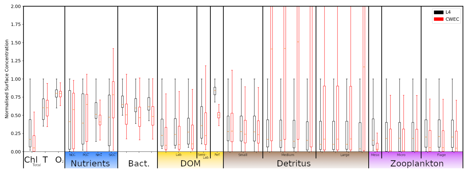
Figure A1 Box and whisker plot showing the 25th, 50th and 75th percentile and upper and lower bound (excluding outliers larger than 1.5× Inter quartile range) of each pelagic marine BGC variable for the RUS scheme in the online testing period. Values for L4 are given in black, and values for the CWEC are given in red. All values are normalised against the upper bound of L4. Chemical components are ordered according to Table 1. The label “T” corresponds to temperature.

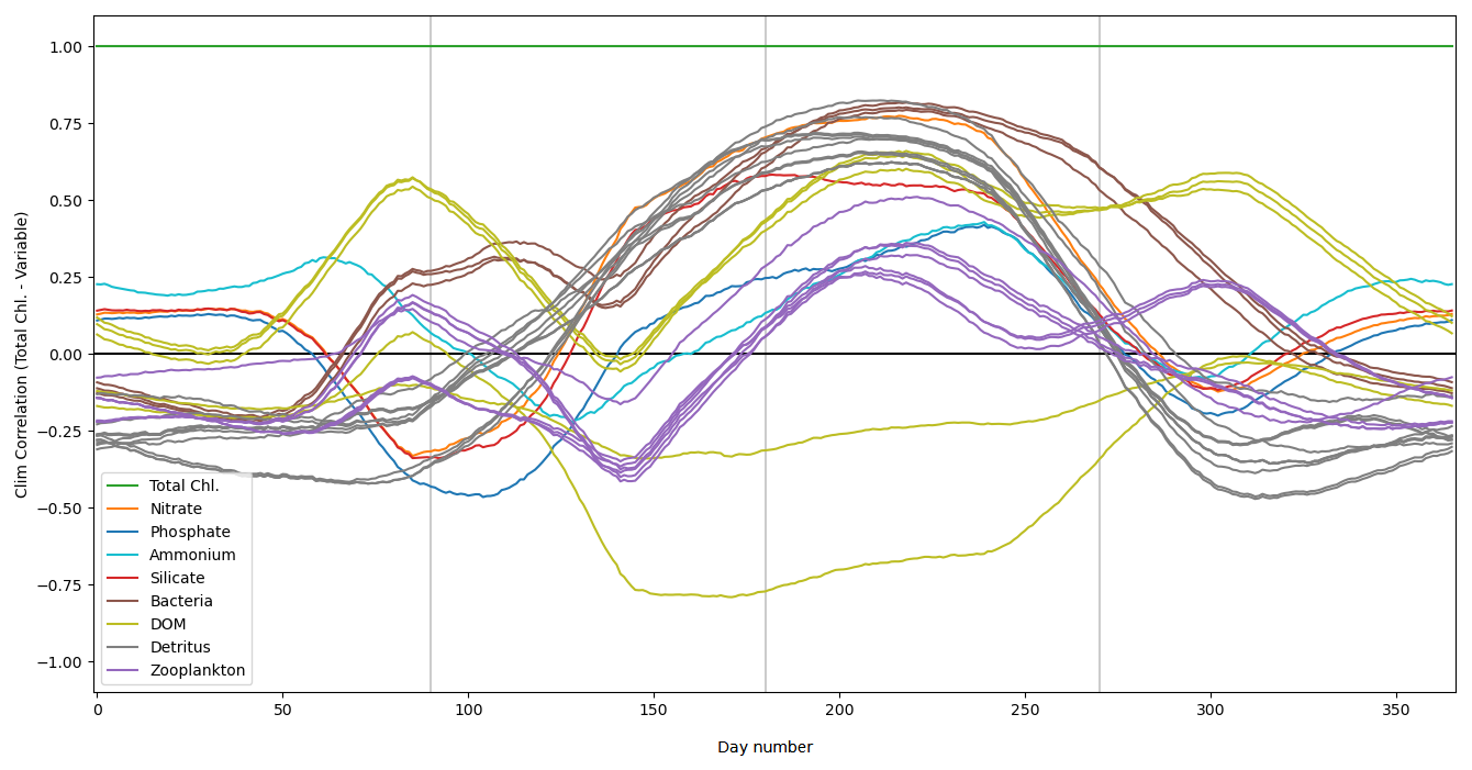
Figure A2 Daily climatological correlations between total chlorophyll and each pelagic variable at the L4 location, calculated from the training free-run period of 2000–2014. Pelagic variables of the same class (according to Table 2) are shown with the same colour, except nutrients (nitrate, phosphate, ammonium and silicate) which are shown with separate colours.

Figure A3 As with Fig.A2, except for the CWEC location from a free-run period of 2000–2010.

Appendix B: Dynamical impact of updating only nitrate

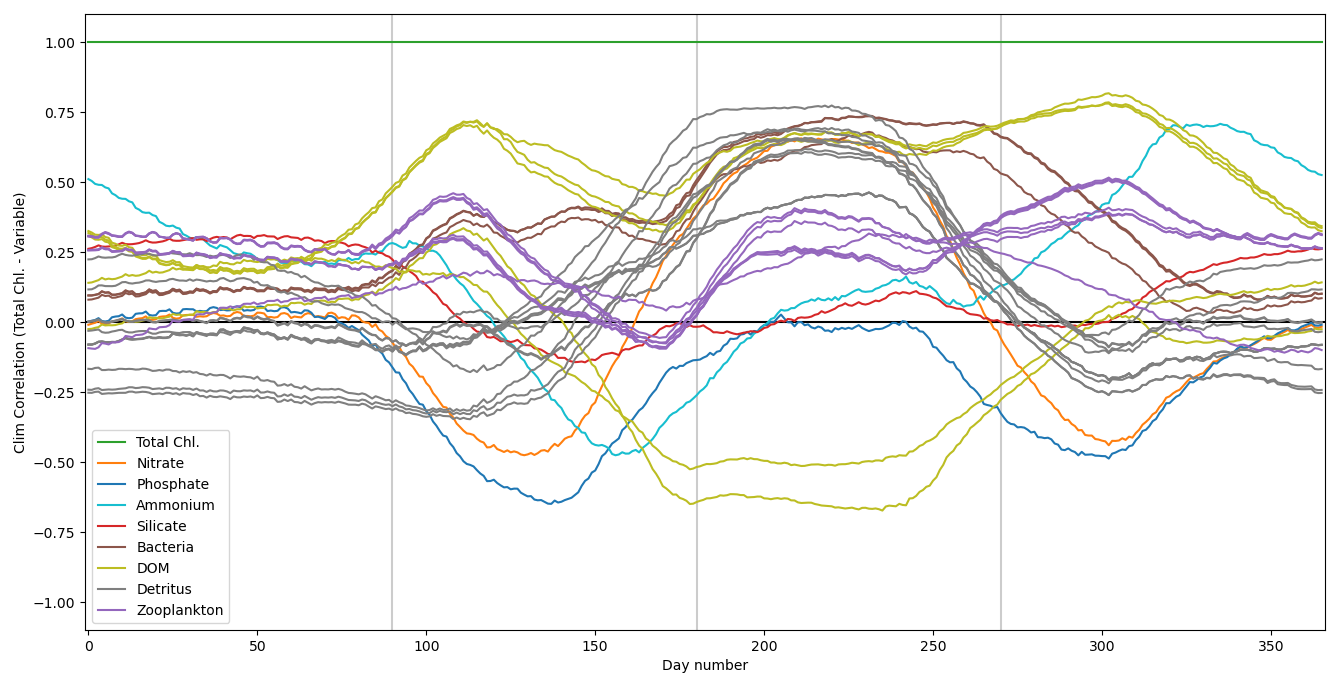
Figure B1 is an extension of Fig. 4, with a representative set of variables that are unobserved and not updated (unlike nitrate which is also unobserved, but updated in this experiment). This clearly shows that the improvement of nitrate does not necessarily translate to an improvement in other variables, regardless of the method used to update the nitrate. This highlights the need to evaluate how different assimilation strategies and variable-update choices affect performance.

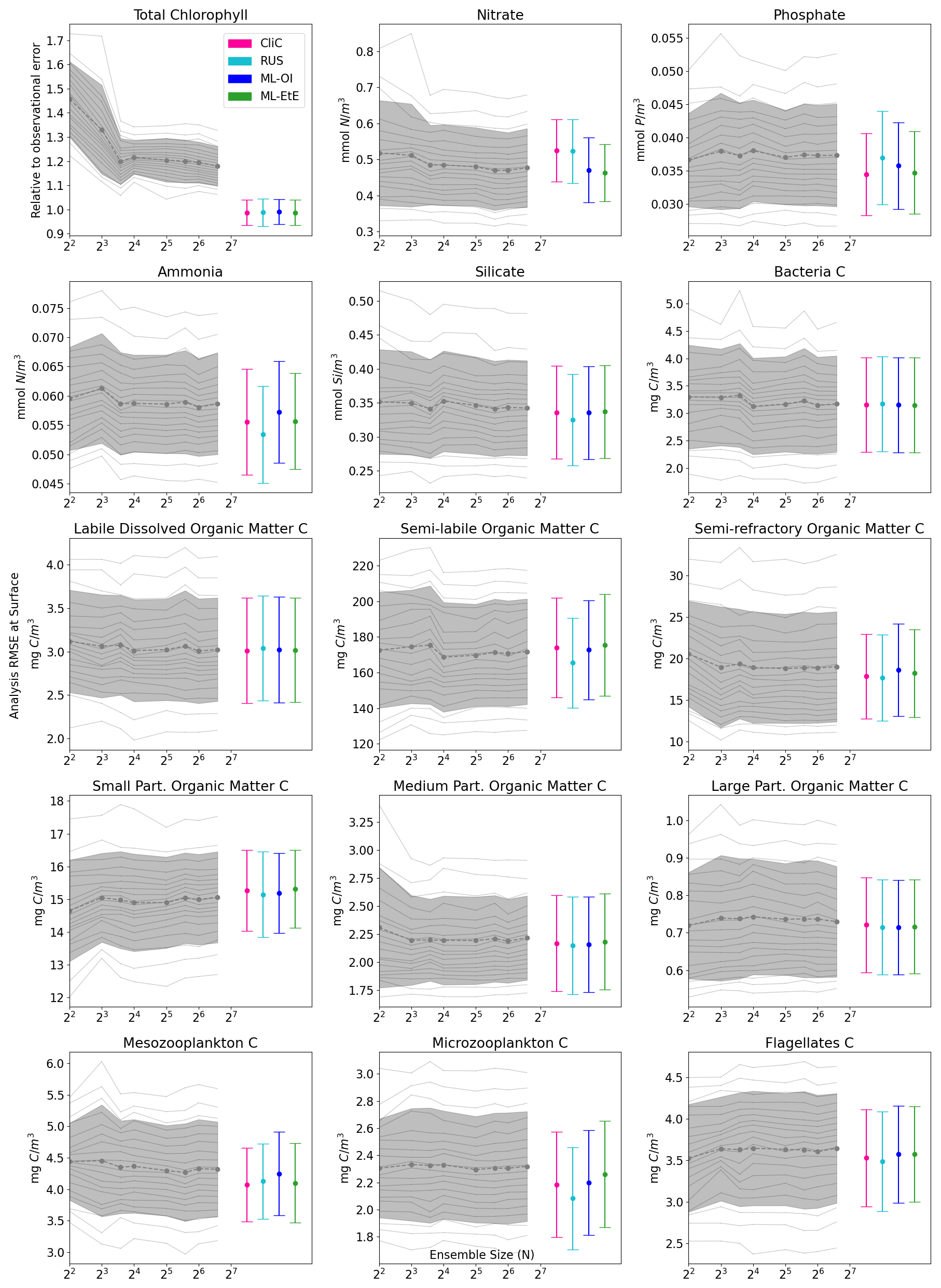
Figure B1 An extension of Fig. 4, where panels for total chlorophyll (observed) and nitrate (unobserved, but updated) are the same. representative set of additional variables (unobserved, not updated) are shown. A “C” indicates the panel is given for the carbon chemical component in the model.