The efficiency and ocean acidification mitigation potential of ocean alkalinity enhancement on multi-centennial timescales

Carbon dioxide removal (CDR) strategies such as ocean alkalinity enhancement (OAE) are likely required in addition to rapid emissions reductions to limit global warming to well below 2 °C. However, the long-term efficiency of OAE and its potential to mitigate climate change and ocean acidification remain uncertain. Here, we investigate efficiencies, climate and ocean acidification responses of idealized OAE using a fully coupled, emission-driven Earth system model across three global warming stabilization scenarios (1.5, 2, and 3 °C) spanning 1861–2500. OAE is implemented as a continuous global surface alkalinity addition of 0.14 Pmol yr⁻¹ following the CDRMIP protocol from 2026 onward. Our results show that OAE reduces atmospheric CO₂ by 73–130 ppm by 2500, with larger reductions under higher warming scenarios and during the first 100 to 200 years of alkalinity addition. In contrast, global surface air temperature decreases nearly linearly by 0.14–0.17 °C per century across all scenarios, indicating that the cooling rate due to OAE is largely insensitive to the emission pathway and background warming level. The interpretation of OAE efficiency depends strongly on the chosen metric. The global gross ocean carbon capture efficiency of about 0.79 remains close to the theoretical maximum, reflecting the negative emissions through OAE, whereas the net ocean capture and atmospheric CO₂ reduction efficiencies are substantially lower and decline over time due to carbon cycle feedbacks in response to lowered atmospheric CO₂. OAE mitigates ocean acidification, at the surface as well as in the interior ocean, with most centennial-scale mitigation arising from atmospheric CO₂ drawdown, an effect shared with other CDR approaches. Direct chemical effects of added alkalinity contribute transiently and diminish over time as the ocean–atmosphere system equilibrates. Overall, our results underscore that rapid emission reductions remain the most effective strategy for achieving the Paris Agreement goals and mitigating ocean acidification.

1 Introduction

Anthropogenic carbon dioxide (CO₂) emissions from fossil fuel combustion and land use change have increased atmospheric CO₂ concentrations by about 50 %, reaching 423 ppm in 2024 (Friedlingstein et al., 2025), higher than at any point in at least the past two million years (IPCC, 2021). This unprecedented increase in greenhouse gas concentrations is the main driver of global surface warming, which averaged about 1.24 °C above pre-industrial levels during 2015–2024 (Forster et al., 2025), and is contributing to more frequent and severe climate extremes both on land and in the ocean (Frölicher et al., 2018; IPCC, 2021). These changes already harm ecosystems and human systems around the world (IPCC, 2022a). Ongoing efforts to reduce emissions remain inadequate and global temperatures are now on track to exceed the 1.5 °C threshold of the Paris Agreement in the next decade.

Limiting global warming to 1.5 °C will require not only deep decarbonization (IPCC, 2022b; Silvy et al., 2024), but also large-scale carbon dioxide removal (CDR), particularly to offset residual emissions from hard-to-abate sectors such as aviation, cement industry and agriculture (IPCC, 2022b; Bossy et al., 2025). As a result, CDR has become an integral component of national pathways to net-zero emissions (Boehm et al., 2023). Current efforts have largely focused on implementing land-based CDR methods, while ocean-based approaches remain comparatively understudied (Smith et al., 2024; Boyd et al., 2025a). Among these, ocean alkalinity enhancement (OAE) stands out as one of the most promising due to its large carbon sequestration potential, long storage timescales, and potential co-benefits of mitigating ocean acidification (Renforth and Henderson, 2017; IPCC, 2021; National Academies of Sciences, Engineering, and Medicine, 2022; Doney et al., 2025). OAE involves adding alkaline materials, such as olivine or quicklime, or alkaline solutions to seawater to enhance its natural ability to absorb atmospheric CO₂. Through this process, aqueous CO₂ is converted into bicarbonate and carbonate ions, which represent longer-lived forms of inorganic carbon in the ocean on centennial to millennial timescales (Renforth and Henderson, 2017; Middelburg et al., 2020; National Academies of Sciences, Engineering, and Medicine, 2022; Ho et al., 2023). On longer timescales, the persistence of the added alkalinity is limited by CaCO₃ sediment interactions and weathering feedbacks (Köhler, 2020; Acksen et al., 2026). The resulting depletion of CO₂ in surface waters drives additional oceanic CO₂ uptake, thereby lowering atmospheric CO₂. In addition, by increasing ocean pH, OAE may help counteract ocean acidification and alleviate stress on marine ecosystems (Doney et al., 2009; Bednaršek et al., 2025).

The feasibility of a CDR approach depends on multiple factors, with efficiency and durability of atmospheric CO₂ reduction being particularly critical. Approaches that fail to achieve substantial and long-lasting removal of atmospheric CO₂ are unlikely to be viable. Efficiency, defined as the amount of additional ocean carbon uptake per unit of alkalinity added, is a key metric for carbon accounting because it determines how much carbon removal can be attributed to an intervention (Boyd et al., 2025b). For OAE, efficiency is shaped by three main factors: the ocean's carbonate chemistry, physical ocean processes and global carbon cycle feedbacks. First, the ocean's carbonate chemistry ultimately limits how much additional atmospheric CO₂ can be taken up and stored as dissolved inorganic carbon in response to added alkalinity, thereby setting the theoretical upper limit of efficiency (Renforth and Henderson, 2017). Second, physical ocean processes such as local mixing and air–sea equilibration dynamics exert a strong control on efficiency (He and Tyka, 2023). For example, if added alkalinity is mixed below the surface before equilibration, efficiency initially decreases (Nagwekar et al., 2024; Zhou et al., 2024). The subducted alkalinity may re-emerge at the surface only much later and far from the deployment site, leading to delayed carbon uptake (Burger et al., 2026). Third, the reduction in atmospheric CO₂ caused by OAE will also reduce oceanic and terrestrial CO₂ uptake, which in turn feeds back on atmospheric CO₂ and reduces efficiency (Schwinger et al., 2024; Jeltsch-Thömmes et al., 2024). Similarly, ocean-internal biogeochemical feedbacks, mostly through calcifying organisms, can influence efficiency (Lehmann and Bach, 2025).

To date, most modelling studies on OAE efficiency have used simplified Earth system models or forced ocean-only configurations (Tyka et al., 2022; He and Tyka, 2023; Nagwekar et al., 2024; Zhou et al., 2024; Martin et al., 2025). Many of these studies prescribe atmospheric CO₂, thereby neglecting changes in oceanic and terrestrial carbon uptake that would result from OAE-induced reductions in atmospheric CO₂, or they focus only on relatively short timescales (decadal to multi-decadal). However, simulations with fully coupled, emission-driven Earth system models are essential to capture the full carbon cycle response, especially over multi-centennial time scales, and its dependence on the background climate state and emissions pathways (Fennel et al., 2023; Palmiéri and Yool, 2024; Schwinger et al., 2024; Lehmann and Bach, 2025; Tyka, 2025). Recently, more fully coupled modelling studies have become available, although the complexity of the models differs. They consistently show that interactions among the atmosphere, ocean, and land biosphere strongly reduce OAE efficiency compared to modelling experiments with prescribed atmospheric CO₂ (Jeltsch-Thömmes et al., 2024; Schwinger et al., 2024; Tyka, 2025; Wey et al., 2025; Sathyanadh et al., 2025; Nagwekar et al., 2026).

Another key knowledge gap concerns the potential of OAE to mitigate ocean acidification, often discussed as a valuable co-benefit of OAE (Bach et al., 2019). Global OAE simulations with other Earth system models indicate a reduction in global and regional ocean acidification (Ilyina et al., 2013; Feng et al., 2016; Mongin et al., 2021; Jin and Cao, 2025), and local real-world experiments show that OAE can enhance pH and support calcification in vulnerable ecosystems such as coral reefs (Albright et al., 2016). However, the magnitude and persistence of OAE-induced pH changes, both globally and regionally, remain uncertain, as previous studies rely on theoretical concepts (van de Mortel et al., 2025) or simplified, coarse-resolution models (Ilyina et al., 2013; Jin and Cao, 2025; Findlay et al., 2025). As with OAE efficiency, addressing these uncertainties requires comprehensive Earth system models capable of capturing global carbon cycle feedbacks (Butenschön et al., 2021; Bednaršek et al., 2025).

In this study, we investigate multiple OAE efficiency metrics and assess the OAE-induced carbon cycle, climate and ocean acidification responses under multi-centennial global warming stabilization scenarios using a comprehensive fully coupled Earth system model. We first describe the model setup and simulation scenarios, followed by the definition of efficiency metrics and the processes governing pH changes. We then assess the climate and carbon cycle response, the temporal and spatial evolution of OAE efficiencies, and the ocean acidification mitigation potential. Finally, we discuss our findings and place it in the context of existing literature.

2 Methods

2.1 GFDL ESM2M model

This study uses the fully-coupled GFDL-ESM2M Earth system model developed at the NOAA Geophysical Fluid Dynamics Laboratory (Dunne et al., 2012, 2013). The individual components of the model are the modular ocean model version MOM4p1 (Griffies et al., 2009), the atmospheric model version AM2 (Anderson et al., 2004), the land model version LM3 (Shevliakova et al., 2009) and the sea-ice model from Winton (2000). The atmosphere and land components have a horizontal resolution of 2° × 2.5°. The ocean model has a horizontal resolution of 1°, which increases to 0.3° near the equator. It has 50 vertical levels, with a layer thickness of 10 m in the upper 200 m gradually increasing to 300 m at greater depths. Additionally, the ocean model is coupled to the biogeochemistry model TOPAZv2, which simulates 30 biogeochemical tracers to represent cycling of carbon and alkalinity, as well as active pelagic calcite and aragonite and their sediment interaction (Dunne et al., 2013). Three phytoplankton groups and implicit zooplankton grazing actively influence the production and remineralisation of carbon and alkalinity. Pelagic calcite and aragonite production depends on the respective saturation state and the associated detritus sinks through the water column and can be dissolved or deposited in the sediments, from where it can either be stored or redissolved. Ocean carbonate chemistry follows routines from the OCMIP2 protocol (Najjar and Orr, 1998). The land model simulates the cycling of carbon, including different vegetation types, soils, wildfires and harvesting.

The model has been shown to perform well in representing the global carbon cycle (Dunne et al., 2013; Bopp et al., 2013; Frölicher et al., 2015; Séférian et al., 2020; Burger et al., 2022). It simulates the uptake and storage of anthropogenic carbon by the marine and terrestrial carbon sinks close to observations (Frölicher et al., 2015; Bronselaer et al., 2017), and it represents alkalinity well by actively simulating both calcite and aragonite cycling in comparison to other climate models (Planchat et al., 2023).

2.2 Simulations setup

A set of different model simulations with and without ocean alkalinity enhancement were performed for this study (Fig. 1). After an initial spin-up (Burger et al., 2020), an emission-driven historical simulation was performed over the period 1861 to 2005, which follows fossil fuel and land-use change CO₂ emissions as well as prescribed non-CO₂ radiative forcing agents from the CMIP5 protocol. This simulation was continued for 20 simulation years in which fossil fuel CO₂ emissions followed observed emissions until 2020 and national determined contributions until 2025 (Friedlingstein et al., 2020; Silvy et al., 2024). From 2026 on, the adaptive emission reduction approach (AERA) was applied to reach a specified global warming level. The AERA algorithm determines the emissions pathway by estimating anthropogenic warming, calculating the forcing-equivalent remaining emissions budget for the prescribed warming target using the transient climate response to cumulative CO₂-forcing-equivalent emissions (TCRE-fe), and then distributing the forcing-equivalent emissions budget over future years according to a third-order polynomial that leads to zero emissions. The timing of net-zero emissions, and thus the time window for reaching the target temperature, is an emergent property of the algorithm rather than an externally imposed constraint. If temperatures overshoot, the AERA responds by prescribing negative emissions. The pathway is recalculated every 5 years based on updated estimates of global mean temperature and the remaining CO₂-forcing-equivalent emission budget at the time of the stocktake (Terhaar et al., 2022). Three target warming levels of 1.5, 2.0 and 3.0 °C above pre-industrial were chosen to cover a range of possible global warming scenarios. These simulations were run until 2500 to investigate changes on multi-centennial timescales under temperature stabilization (labelled as “Ref” in figures). Non-CO₂ radiative forcing agents and land-use change were following the RCP2.6 scenario after 2005 in all future warming simulations and are kept constant after 2100 (Silvy et al., 2024).

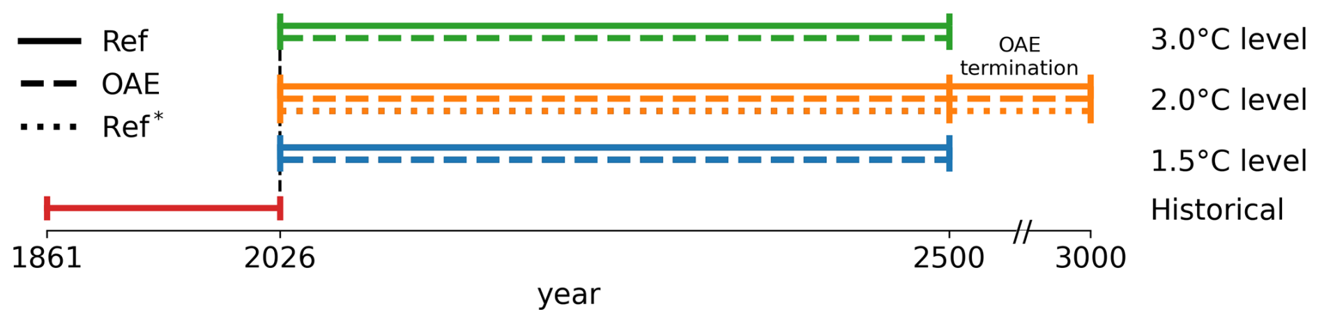
Figure 1 Schematic overview of all simulations conducted in this study. All simulations are branched in 2026 from simulations that follow historical fossil fuel and land-use change CO₂ emissions along with other non-CO₂ radiative forcing agents. The reference simulations (Ref) stabilize global surface air temperature at 1.5, 2 and 3 °C following the adaptive emission reduction approach and have no ocean alkalinity enhancement (OAE). Corresponding OAE simulations follow the same emission pathways that would lead to stabilization, but include alkalinity enhancement. An additional 2 °C reference simulation (Ref^∗) follows prescribed atmospheric CO₂ from the OAE 2 °C simulation, but without OAE. Each configuration is run with 5 ensemble members each. All these simulations are run until 2500. Additionally, one member of the set of 2 °C simulations is extended until 3000, but with OAE termination in 2500.

The Ocean Alkalinity Enhancement (OAE) experiments follow the same CO₂ emission and non-CO₂ forcing pathways as the reference simulations (labelled as “OAE” in figures). OAE is implemented following the protocol defined by the Carbon Dioxide Removal Model Intercomparison Project (CDRMIP) (Keller et al., 2018b). Additional CO₂ emissions due to the OAE intervention, associated with the mining, processing, and transport of alkaline materials or solutions (Foteinis et al., 2022), are not included in this study. A total of 0.14 Pmol yr⁻¹ of alkalinity is continuously and homogeneously added to the global surface ocean, excluding regions south of 60° S and north of 70° N, as they are seasonally sea-ice covered and therefore a year-round input of alkalinity to the surface ocean may not be possible. Although this magnitude and spatial distribution of alkalinity input is unlikely to be achievable with current or near-future societal means (Eisaman et al., 2023), it provides a useful framework for exploring impacts of global-scale OAE and facilitates comparison with other model-based studies using the same framework (Keller et al., 2018b; Köhler, 2020; Qu et al., 2025; Wey et al., 2025).

Following the approach of Schwinger et al. (2024), we perform a third set of simulations to assess feedback processes that influence the efficiency of OAE (labelled as “Ref^∗” in figures). These simulations are driven by prescribed atmospheric CO₂ concentrations from the “OAE” run (which are lower than in the REF run) and therefore simulate the same climate trajectory as the “OAE” simulations, but without the addition of the alkalinity. The non-CO₂ forcing is the same as in the OAE and Ref simulations. The simulations thus exclude any additional atmospheric CO₂ removal by the ocean due to OAE. These additional simulations help to isolate the OAE effect by removing global carbon feedback processes. We conducted those simulations only for the 2 °C warming level, as it is sufficient to illustrate the relevant processes, which can be generalized to other warming levels.

For all scenarios, we have conducted a five-member perturbed initial-condition ensemble. An initial-condition ensemble enables the separation of the forced climate response from uncertainties arising from natural internal variability (Frölicher et al., 2009; Deser et al., 2020). We set up the ensembles with a sea surface temperature perturbation on the order of 10⁻⁵ °C at one grid point in the Weddell Sea on 1 January 1861 (Burger et al., 2020; Frölicher et al., 2020).

To investigate the effect of OAE termination on both the efficiencies and the ocean acidification response, we extended one ensemble member of the 2 °C OAE simulations to the year 3000, but terminating OAE in 2500, and extended both reference simulations as well.

2.3 Definitions of OAE efficiencies

Several complementary metrics can be used to assess OAE efficiency, each capturing different aspects. These metrics are explained in the following and illustrated, along with the associated carbon fluxes, in Fig. 2.

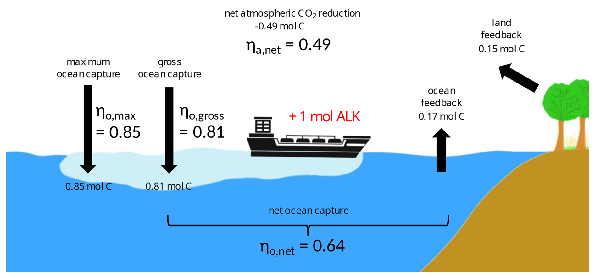
Figure 2 Schematic illustration of OAE efficiency metrics and associated carbon transfer of adding, for example, 1 mol of alkalinity to the surface ocean. The carbon transfer per added alkalinity are the ensemble average of the first 100 years in the 2 °C simulation. The metrics include maximum ocean capture efficiency η_o,max, net ocean capture efficiency η_o,net, gross ocean capture efficiency η_o,gross and net atmospheric CO₂-reduction η_a,net.

2.3.1 Maximum ocean capture efficiency

The maximum ocean capture efficiency η_o,max of OAE is derived purely from the carbonate chemistry of seawater. It represents the change in dissolved inorganic carbon (DIC) resulting from the addition of alkalinity (ALK), assuming the oceanic pCO₂ fully re-equilibrates to the pCO₂ before alkalinity addition and is calculated at the ocean surface (Frankignoulle et al., 1994; Renforth and Henderson, 2017; Tyka et al., 2022). It can be expressed as the ratio of the sensitivity of the seawater partial pressure of CO₂ (pCO₂) to changes in alkalinity versus its sensitivity to changes in dissolved inorganic carbon (DIC):

$$\begin{array}{}\text{(1)}& {\mathit{\eta }}_{\mathrm{o},\text{max}}=-{\displaystyle \frac{\partial p{\mathrm{CO}}_{\mathrm{2}}}{\partial \text{ALK}}}/{\displaystyle \frac{\partial p{\mathrm{CO}}_{\mathrm{2}}}{\partial \text{DIC}}}\end{array}$$

We use MOCSY to calculate sensitivities of the oceans' pCO₂ to dissolved inorganic carbon and alkalinity with units of $\mathrm{\mu }\mathrm{atm}(\mathrm{mol}{\mathrm{kg}}^{-\mathrm{1}}{)}^{-\mathrm{1}}$ (Orr and Epitalon, 2015). A η_o,max value of 0.8 indicates that an addition of 1 mol kg⁻¹ of alkalinity can potentially increase ocean carbon content by 0.8 mol kg⁻¹.

2.3.2 Net ocean capture efficiency

We quantify the net ocean capture efficiency η_o,net, which accounts for both the ocean's feedback to the OAE-induced reduction of atmospheric CO₂ and the horizontal and vertical redistribution of added alkalinity by physical ocean processes before full equilibration with the atmosphere (Schwinger et al., 2024). The atmospheric CO₂ is also influenced by the land carbon feedback (i.e. reduced terrestrial CO₂ uptake due to lower atmospheric CO₂), buffering part of the OAE-induced reduction in atmospheric CO₂ (Keller et al., 2014, 2018a). The net ocean capture efficiency η_o,net is defined as the ratio of the change in air–sea CO₂ flux to the amount of alkalinity added:

$$\begin{array}{}\text{(2)}& {\mathit{\eta }}_{\mathrm{o},\text{net}}={\displaystyle \frac{F_{{\mathrm{CO}}_{\mathrm{2}}}^{\text{OAE}}-F_{{\mathrm{CO}}_{\mathrm{2}}}^{\mathrm{Ref}}}{F_{\mathrm{ALK}}}}\end{array}$$

Here, $F_{{\mathrm{CO}}_{\mathrm{2}}}$ refers to the air–sea CO₂ flux in Pmol yr⁻¹. The numerator represents the additional CO₂ uptake by the ocean in the “OAE” simulation relative to the reference simulation “Ref”, both following the same emissions trajectory. F_ALK denotes the rate of alkalinity addition of 0.14 Pmol yr⁻¹. Efficiencies are calculated for each ensemble member individually and are based on annual mean carbon fluxes. Different to how net efficiency is defined here, this term sometimes also refers to the OAE efficiency including life-cycle emissions (Foteinis et al., 2022; Delval et al., 2025; Katish et al., 2026).

2.3.3 Gross ocean capture efficiency

To quantify the carbon flux resulting solely from alkalinity addition and the redistribution of added alkalinity by physical ocean processes before equilibration with the atmosphere, excluding the ocean and land carbon feedbacks in response to the OAE-induced reduction of atmospheric CO₂, we define the gross ocean capture efficiency, η_o,gross (Schwinger et al., 2024; Zhou et al., 2024; Tyka, 2025):

$$\begin{array}{}\text{(3)}& {\mathit{\eta }}_{\mathrm{o},\text{gross}}={\displaystyle \frac{F_{{\mathrm{CO}}_{\mathrm{2}}}^{\mathrm{OAE}}-F_{{\mathrm{CO}}_{\mathrm{2}}}^{{\mathrm{Ref}}^{\ast }}}{F_{\mathrm{ALK}}}}\end{array}$$

It is calculated by subtracting the air–sea CO₂ flux of the Ref^∗ simulation from that of the OAE simulation, and dividing the result by the amount of alkalinity added in the OAE simulation. The Ref^∗ simulation shares the same climate state as the OAE simulation, but oceanic CO₂ uptake is not driven by OAE. The difference between the OAE and Ref^∗ simulations eliminates the natural carbon fluxes and feedback processes between reservoirs, thereby leaving the total additional ocean carbon uptake due to OAE. We did an extra experiment to verify that this additional ocean carbon uptake leads to the same reduction in atmospheric CO₂ as direct air capture (Appendix A) and it therefore represents negative emissions.

2.3.4 Net atmospheric CO₂ reduction efficiency

The fourth efficiency metric used in this study is the net atmospheric CO₂ reduction efficiency η_a,net:

$$\begin{array}{}\text{(4)}& {\mathit{\eta }}_{\mathrm{a},\text{net}}={\displaystyle \frac{R_{{\mathrm{CO}}_{\mathrm{2}}}^{\mathrm{OAE}}-R_{{\mathrm{CO}}_{\mathrm{2}}}^{\mathrm{Ref}}}{F_{\mathrm{ALK}}}}\end{array}$$

It describes the difference between the change in atmospheric CO₂ inventory per year ($R_{{\mathrm{CO}}_{\mathrm{2}}}$ in Pmol yr⁻¹) between the OAE simulation and the Ref simulation divided by the yearly addition of alkalinity (Jeltsch-Thömmes et al., 2024; Tyka, 2025). This metric describes the potential of OAE to reduce atmospheric CO₂ and thereby influence global warming.

2.4 Drivers of ocean acidification mitigation

Three processes drive the total pH response to OAE: reduction in atmospheric CO₂, the pH change at the new pCO₂ equilibrium, and the remaining pCO₂ disequilibrium:

$$\begin{array}{}\text{(5)}& \mathrm{\Delta }{\text{pH}}_{\text{total}}\simeq \mathrm{\Delta }{\text{pH}}_{\text{CDR}}+\mathrm{\Delta }{\text{pH}}_{\text{equilibrated}}+\mathrm{\Delta }{\text{pH}}_{\text{disequilibrium}}\end{array}$$

The three processes are described in the following.

2.4.1 Reduction in atmospheric CO₂

Any CDR method that lowers atmospheric CO₂, being terrestrial or marine, mitigates ocean acidification, as seawater loses carbon when equilibrating to the lowered atmospheric pCO₂. This CDR-driven pH increase can be quantified using the Ref^∗-simulation, which follows the atmospheric CO₂ trajectory of the OAE simulation, but excludes alkalinity addition. The resulting pH difference relative to the Ref-simulation represents the pH change due to CDR:

$$\begin{array}{}\text{(6)}& \mathrm{\Delta }{\text{pH}}_{\text{CDR}}={\text{pH}}^{{\mathrm{Ref}}^{\ast }}-{\text{pH}}^{\text{Ref}}\end{array}$$

2.4.2 Equilibrated pH response

The sensitivities of pCO₂ and pH to changes in dissolved inorganic carbon (DIC) and total alkalinity differ. When oceanic pCO₂ is lowered through alkalinity addition and subsequently returns to the original value through air–sea carbon uptake, both alkalinity and DIC are higher than before alkalinity addition. As a result, the pH is higher than before the intervention. We refer to this as the “pH-equilibrated” effect, where identical pCO₂ levels correspond to different carbonate system and pH states before and after alkalinity addition. Research about the ecosystem impact of OAE often distinguishes between equilibrated and un-equilibrated OAE (Hartmann et al., 2023). Equilibrated OAE assumes that the alkaline solution added to the ocean has already re-equilibrated with the atmosphere and taken up CO₂ according to the maximum ocean capture efficiency, characterized by the equilibrated pH response. Un-equilibrated OAE assumes that pCO₂ is not yet back to equilibrium with the atmosphere, and the pH response is here characterized by the equilibrated pH response together with the pCO₂ disequilibrium effect (described below). The contribution of the equilibrated pH response can be estimated from the ocean carbonate system and the alkalinity perturbation relative to the reference state (full derivation in Appendix B):

$$\begin{array}{}\text{(7)}& \mathrm{\Delta }{\text{pH}}_{\text{equilibrated}}\simeq {\mathit{\eta }}_{\mathrm{o},\text{max}}{\displaystyle \frac{\mathrm{\Delta }\text{ALK}}{{\mathrm{ALK}}^{\mathrm{Ref}}}}{\displaystyle \frac{\mathrm{1}}{\ln \left(\mathrm{10}\right)}}\end{array}$$

2.4.3 pCO₂ disequilibrium

During oceanic pCO₂ equilibration with the atmosphere after alkalinity addition, the temporarily lower pCO₂ in seawater leads to an increase in pH. We can quantify this contribution by manipulating the ocean carbonate system offline. We use the oceanic conditions from the OAE simulation (i.e. alkalinity, pCO₂, temperature, salinity, phosphate and silicate concentrations), where pCO₂ in the ocean remains depressed because re-equilibration with the atmosphere is incomplete. The offset in oceanic pCO₂ is calculated as the difference between the OAE and Ref^∗-simulation: $\mathrm{\Delta }p{\mathrm{CO}}_{\mathrm{2}}=p{\mathrm{CO}}_{\mathrm{2}}^{{\mathrm{Ref}}^{\ast }}-p{\mathrm{CO}}_{\mathrm{2}}^{\mathrm{OAE}}$, which isolates the effect of alkalinity addition since both simulations share the same atmospheric CO₂. We then recompute the carbonate system for OAE conditions but add ΔpCO₂ to restore full air–sea equilibrium using the pyCO2SYS package (Humphreys et al., 2022). This yields the carbonate system state after equilibration (i.e., when ΔpCO₂=0). The pH change associated with the pCO₂ disequilibrium is then given by:

$$\begin{array}{}\text{(8)}& \mathrm{\Delta }{\text{pH}}_{\text{Disequilibrium}}={\text{pH}}^{\text{OAE}}-{\text{pH}}^{\text{OAE}+\mathrm{\Delta }p{\mathrm{CO}}_{\mathrm{2}}}\end{array}$$

3 Results

3.1 Atmospheric CO₂ and global temperature response

In the Ref simulations without OAE, global surface air temperature stabilizes at the prescribed global warming levels (solid lines in Fig. 3a). In each case, CO₂ emissions decline to zero and subsequently become slightly negative (Fig. C1), which is required to maintain the stabilized warming levels through the year 2500, as the GFDL-ESM2M model has a positive zero emission commitment on multi-centennial timescales (Frölicher et al., 2014; Frölicher and Paynter, 2015; Silvy et al., 2024). The 31 year mean atmospheric CO₂ concentration peaks at 484 ppm [455–504] in 2074 [2052–2102] in the 1.5 °C scenario, at 573 ppm [551–589] in 2096 [2081–2112] in the 2 °C scenario and at 758 ppm [742–777] in 2176 [2164–2186] in the 3 °C scenario (Fig. 3b). Thereafter, atmospheric CO₂ decreases due to the continuous uptake of carbon by the terrestrial biosphere and predominately by the ocean.

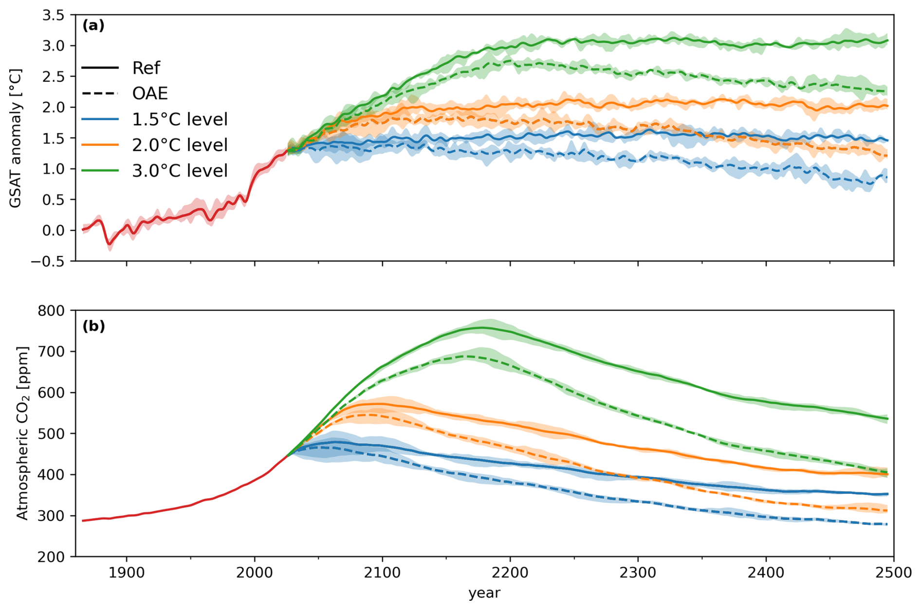
Figure 3 Global surface air temperature anomalies (a) and atmospheric CO₂ (b) over 1861 to 2500 under three different global warming stabilization scenarios with and without OAE. Red lines show the 1861–2025 historical period. Solid lines are the reference simulation (Ref) and dashed lines are simulations with ocean alkalinity enhancement (OAE). All lines are ensemble and 31 year running means, while the shading represents the ensemble range.

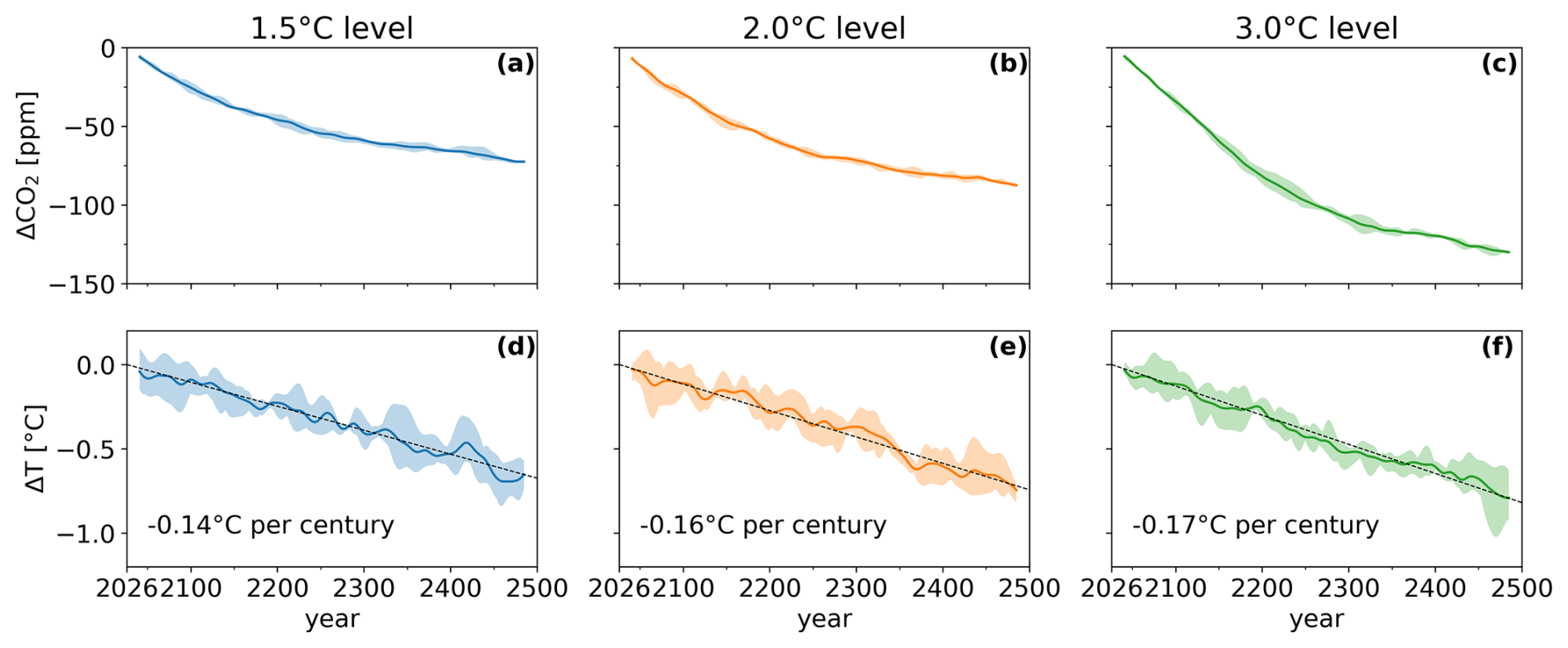
Figure 4 Difference in annual mean atmospheric CO₂ (a–c) and global surface air temperature (d–f) between the ocean alkalinity enhancement (OAE) and reference (Ref) simulations over time for the three global warming stabilization scenarios 1.5 °C (a, d), 2 °C (b, e) and 3 °C (c, f). All lines are ensemble and 31 year running means, while the shading represents the ensemble range. Dashed black lines in (d–f) show the linear trend and its estimates are noted.

In the OAE simulations, the continuous addition of alkalinity to the surface ocean causes additional carbon uptake from the atmosphere and reduces atmospheric CO₂ concentrations compared to the reference simulations without OAE (dashed lines in Fig. 3b). The 31 year mean peak atmospheric CO₂ is lower and earlier with OAE than without on the ensemble average, albeit with overlapping ensemble ranges: at 468 ppm [437–488] in year 2059 [2041–2088] in the 1.5 °C scenario, at 546 ppm [524–560] in year 2085 [2076–2097] in the 2 °C scenario and at 689 ppm [677–708] in year 2167 [2158–2178] in the 3 °C scenario. The decrease in atmospheric CO₂ increases with the amount of global warming. Atmospheric CO₂ concentrations are 73 ppm [72–74] lower in the 1.5 °C scenario, 88 ppm [86–88] lower in the 2 °C scenario, and 130 ppm [130–131] lower in the 3 °C scenario relative to their respective reference simulations between 2470 and 2500 (Fig. 4a–c). The greatest reductions occur within the first 100 (1.5 °C scenario) to 200 (3 °C scenario) years following the start of alkalinity addition (Fig. 4a–c), after which the differences increase less towards the end of the simulations (explained in Sect. 3.3).

The reduction in atmospheric CO₂ under OAE reduces global surface air temperature relative to the reference scenarios (Fig. 3a). Global surface air temperature is 0.64 °C [0.57–0.71] lower in the 1.5 °C scenario, 0.75 °C [0.68–0.80] lower in the 2 °C scenario, and 0.79 °C [0.65–0.96] lower in the 3 °C scenario compared to their respective references between 2470 and 2500. Unlike atmospheric CO₂ concentrations, which showed the largest differences developing shortly after alkalinity addition, the surface temperature difference increases approximately linearly throughout the simulation in all scenarios (Fig. 4d–f). In the 2 °C scenario, the global surface air temperature decreases linearly by −0.16 °C per century [−0.15 to −0.17]. The temperature trend is slightly lower for the 1.5 °C scenario with a cooling of −0.14 °C per century [−0.13 to −0.15] and largest in the 3 °C scenario with −0.17 °C per century [−0.16 to −0.19]. This near-linear trend reflects the logarithmic relationship between radiative forcing and CO₂. Using the formulation of Myhre et al. (1998), ΔF = −5.35 W m⁻² $\ln ({\mathrm{CO}}_{\mathrm{2}}^{\mathrm{Ref}}/{\mathrm{CO}}_{\mathrm{2}}^{\mathrm{OAE}})$, we estimate a near-linear reduction in radiative forcing of −0.29 to −0.34 W m⁻² per century (R² > 0.95 for all scenarios) with a higher reduction in higher warming levels. The trends in radiative forcing show only small variations between scenarios, even though the reductions in atmospheric CO₂ concentrations due to OAE differ much more. This is due to similar ratios of CO₂ between the reference scenario and the OAE simulations across warming levels, but slightly higher for a warmer climate. Consequently, the three scenarios exhibit comparable cooling trends despite their differing CO₂ trajectories, although the exact temperature response may also be influenced by scenario-dependent climate feedbacks and ocean heat uptake.

The regional temperature response to global OAE deployment (Fig. C2a–c) closely mirrors the spatial pattern of greenhouse gas-induced warming (cf. Fig. 4.19 in Lee et al., 2021), but with the opposite sign. Cooling is strongest over continents and at high northern latitudes, and weaker over the ocean, particularly in the Southern Ocean. An exception to the overall cooling occurs in the northern North Atlantic, where a localized warming develops in the higher warming scenarios. This North Atlantic warming reflects an earlier and stronger recovery of the Atlantic Meridional Overturning Circulation under OAE, which enhances ocean heat transport into the region (not shown). This effect is most pronounced in the 3 °C scenario.

3.2 Global carbon flux response

Ocean alkalinity enhancement substantially increases the oceans' alkalinity inventory (Fig. C3). The added alkalinity in turn leads to additional ocean carbon uptake and lowers atmospheric CO₂, but part of this drawdown is offset by carbon release from the land biosphere (Fig. 5). In the reference simulations, the total cumulative ocean carbon uptake since pre-industrial increases rapidly initially with increasing CO₂ emissions and slows markedly toward the end of the simulation when emissions reach near-zero or become negative (solid blue lines in Fig. 5). OAE leads to a persistent additional increase in cumulative ocean carbon uptake relative to the reference scenario (dashed blue lines in Fig. 5). By year 2500, cumulative ocean carbon uptake is higher by 362 PgC [356–366], 380 PgC [377–383] and 407 PgC [403–412] in the 1.5, 2, and 3 °C scenarios, respectively. When feedbacks that redistribute carbon among reservoirs are neglected, the cumulative ocean uptake is substantially larger. In the 2 °C scenario, this gross cumulative ocean carbon uptake attributable to OAE (the difference between OAE and Ref^∗) amounts to 628 PgC [625–632], approximately 65 % larger than the net uptake. This difference arises because reduced atmospheric CO₂ concentrations due to OAE result in an anomalous outgassing of carbon stored in the ocean, thereby offsetting the gross ocean carbon uptake due to OAE. The reduction in atmospheric CO₂ is modulated by anomalous carbon release from the land biosphere. Note that the historical carbon release from land is due to land-use change emissions, which dominate over the land carbon uptake due to increases in atmospheric CO₂ (Silvy et al., 2024). In the 2 °C scenario, this land carbon release totals 194 PgC [189–198], resulting in a net atmospheric carbon reduction of 189 PgC [185–192]. The land carbon response varies across warming levels. The net carbon release from land is largest in the 1.5 °C scenario at 209 PgC [196–218] and smallest in the 3 °C scenario at 129 PgC [122–134]. Consequently and following the ocean carbon uptake, the net atmospheric CO₂ reduction is largest in the 3 °C scenario (279 PgC [271–284]) and smallest in the 1.5 °C scenario (156 PgC [149–164]).

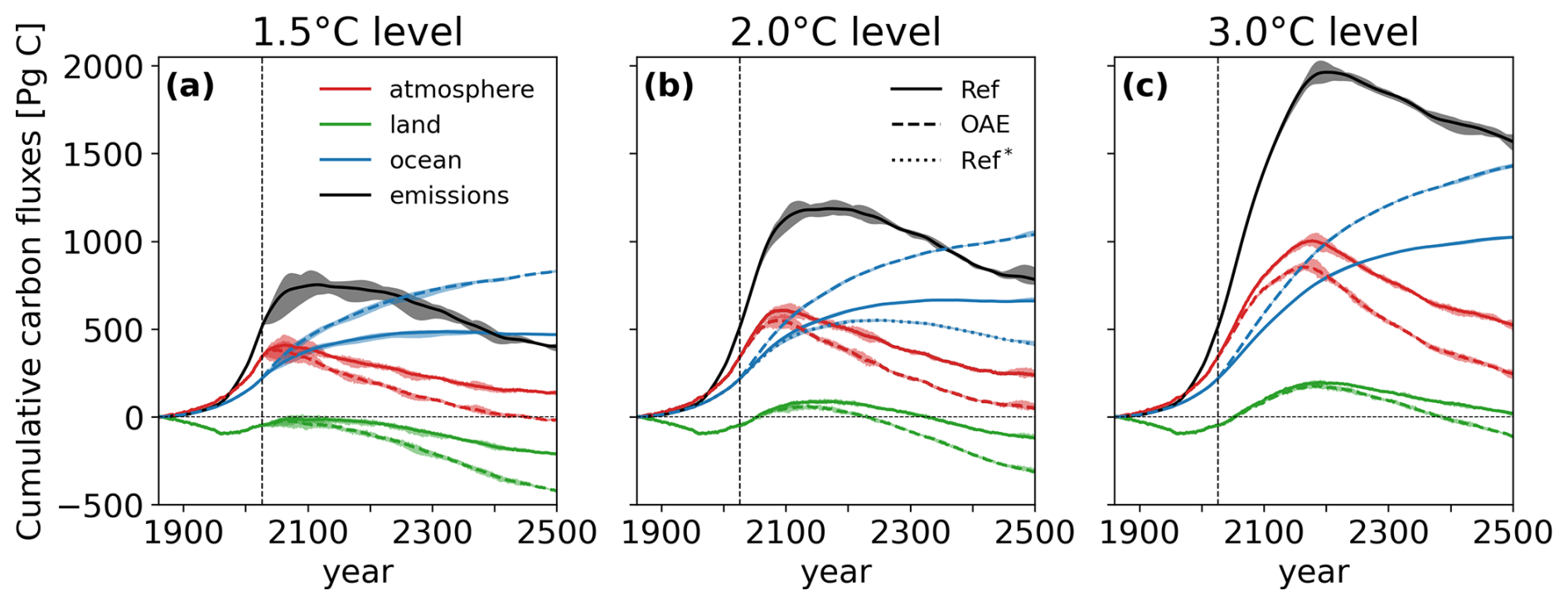
Figure 5 Cumulative globally integrated carbon fluxes since pre-industrial for the atmosphere (red), land (green, including land-use changes), and ocean (blue), as well as fossil fuel CO₂ emissions (black) for the reference simulations (Ref), ocean alkalinity enhancement (OAE) and the additional reference simulation (Ref^∗) under the 1.5, 2 and 3 °C (a–c) global warming scenarios. The dashed vertical black lines indicate the start year of OAE deployment. All lines show ensemble means and shading indicates the ensemble range.

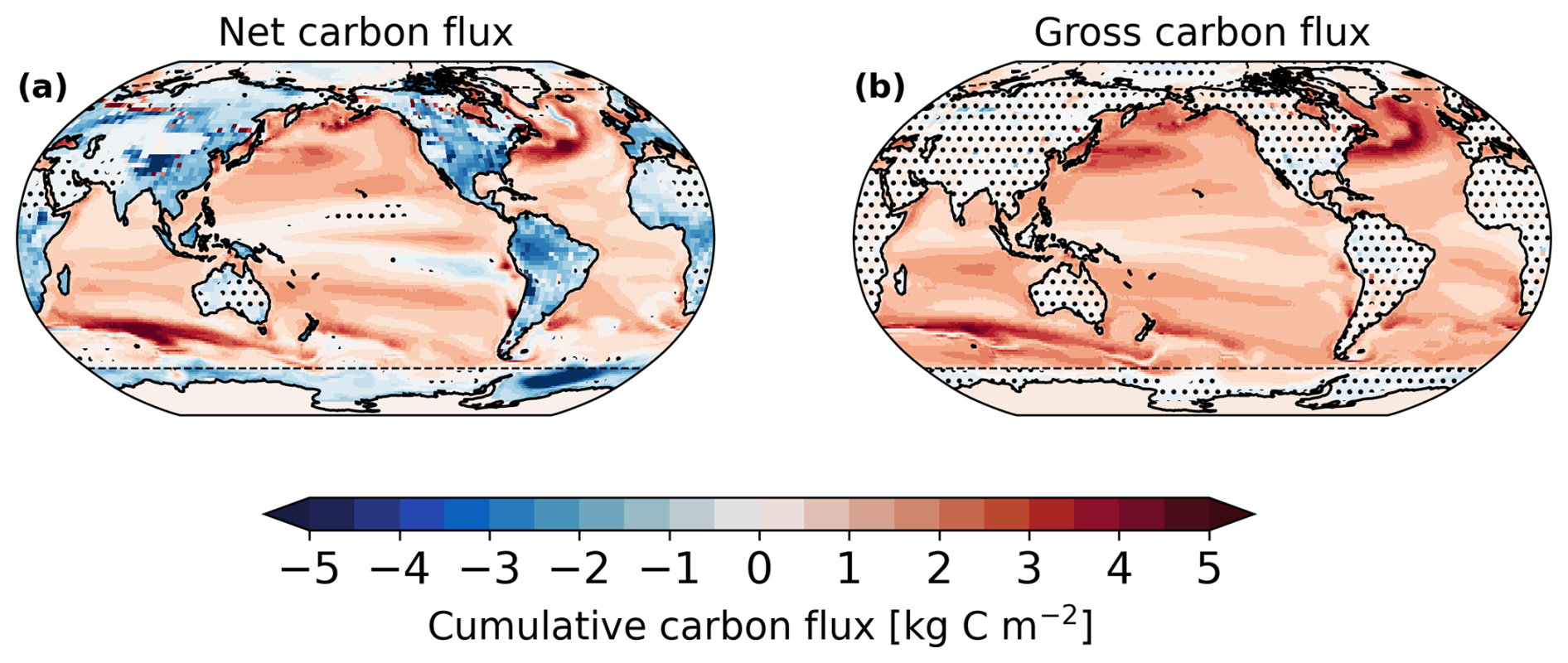
Figure 6 Spatial maps of cumulative net carbon fluxes (difference between OAE and Ref simulation) from 2026 to 2500 for the 2 °C warming scenario in (a) and the gross carbon fluxes (difference between OAE and Ref^∗) in (b). Positive indicates additional ocean carbon uptake. Colours show ensemble means and hatchings show differences that are not significant at the 95 % confidence level based on a two-sided Students t-test. Dashed black lines mark the regions north of 70° N and south of 60° S, where alkalinity addition is not applied.

Regionally, OAE leads to enhanced cumulative net carbon uptake in most ocean regions (Fig. 6a), with particularly strong uptake along western boundary currents and north of the Antarctic Circumpolar Current. However, some regions become anomalous cumulative carbon sources over time (i.e., these regions lose carbon to the atmosphere relative to the reference simulation without OAE). Most notably, the Southern Ocean south of 60° S shows net outgassing, as no alkalinity is added in these regions and the lower atmospheric CO₂ leads to anomalous outgassing. A similar signal emerges south of the eastern tropical Pacific. There, added alkalinity produces only a weak local reduction in ocean pCO₂ due to high buffer capacity and low accumulation of alkalinity, while atmospheric pCO₂ is reduced more strongly by global OAE, leading to a negative air–sea pCO₂-gradient and hence outgassing in these regions. The land biosphere exhibits widespread carbon loss, with strong spatial variability in magnitude (Fig. 6a). The gross cumulative ocean carbon uptake attributable to OAE (difference between OAE and Ref^∗) is positive everywhere (Fig. 6b) and closely resembles the spatial pattern of cumulative anthropogenic carbon uptake (Frölicher et al., 2015). Spatial uptake patterns are relatively uniform during the first century but become increasingly heterogeneous over time. As the atmospheric CO₂ levels in the REF^∗ and OAE simulations are identical, the land shows no significant changes in carbon fluxes (Fig. 6b).

3.3 Ocean alkalinity enhancement efficiency

The simulated carbon cycle response and differences between warming levels relate to the efficiency of OAE. The four metrics to assess the global efficiency of OAE (Sect. 2.3) differ strongly in their absolute values, temporal evolution, and sensitivity to the global warming stabilization level and emission pathway (Fig. 7). The maximum ocean capture efficiency at the surface, determined solely by the response of seawater carbonate chemistry to alkalinity addition, remains nearly constant over time and across the three warming levels at 0.81–0.86 (black lines in Fig. 7). However, it increases slightly at higher atmospheric CO₂, where the ocean buffer capacity is reduced (Fig. C4). At lower buffer capacities, the sensitivity of ocean pCO₂ to changes in alkalinity increases relative to that with respect to dissolved inorganic carbon, allowing for an increased uptake of carbon to balance an alkalinity-induced reduction of pCO₂. As a result, efficiencies are slightly higher at peak atmospheric CO₂ and in the 3.0 °C scenario compared to the 1.5 °C case.

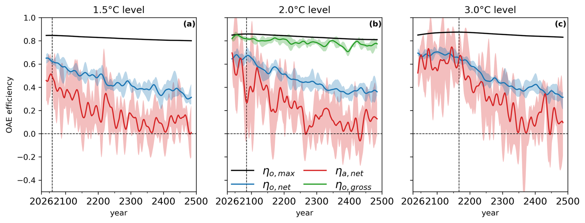
Figure 7 Annual efficiencies of ocean alkalinity enhancement for the three global warming stabilization scenarios 1.5, 2 and 3 °C (a–c). Maximum ocean capture efficiency η_o,max in black, net ocean capture efficiency η_o,net in blue, net atmospheric CO₂-reduction η_a,net in red and gross ocean capture efficiency η_o,gross in green. Dashed vertical black lines indicate the ensemble average year of peak atmospheric CO₂. All lines are ensemble and 31 year running means, while the shading represents the ensemble range.

The net ocean capture efficiency, defined as the change in net air–sea CO₂ flux per unit of alkalinity added, is consistently lower than the maximum efficiency and declines over time (blue lines in Fig. 7). Before peak atmospheric CO₂, efficiencies range between 0.64–0.68 with little variation between scenarios, but slightly higher in warmer scenarios. After the peak, they drop to 0.35–0.36 by 2400–2500, reflecting a gradual long-term decrease. This temporal decline is a result of four interacting processes that are qualitatively discussed: the redistribution of alkalinity within the ocean interior, changes in the ocean buffer capacity, carbon effluxes from the land biosphere and ocean internal changes of alkalinity and DIC by biological activity. First, the added alkalinity undergoes vertical mixing and thereby, the volume in exchange with the atmosphere, over which the equilibration with the atmosphere occurs, increases steadily over time. The larger the volume, the more old carbon-rich waters are being upwelled to the surface and see an atmosphere with reduced atmospheric CO₂ concentration, resulting in anomalous outgassing to the atmosphere and hence lowering net ocean carbon uptake. We use the effective mixed layer depth for OAE from Zhou et al. (2024), characterizing the ocean volume under influence of alkalinity addition. Note that this is not the depth of the commonly used wind-driven mixed layer. Scenarios show negligible differences in magnitude and temporal change in this volume, with the effective mixed layer depth increasing near-linearly from around 140 m in 2026 to about 1400 m in 2500 (not shown), leading to a steady decrease in efficiency. Second, a low ocean buffer capacity means that the change in oceanic pCO₂ per change in dissolved inorganic carbon is large compared to the sensitivity of atmospheric pCO₂ to the atmospheric carbon content. In this case, a lot of carbon is taken up by the ocean until both systems equilibrate at an intermediate pCO₂ and efficiency is high. The buffer capacity is lower in the high warming scenarios and decreases before peak atmospheric CO₂ and increases afterwards in each scenario (Fig. C4). As the timing of peak CO₂ differs between scenarios, so does the influence of buffer capacity onto the efficiency. Third, the reduction in atmospheric CO₂ by ocean carbon uptake is buffered by a relative efflux of carbon from the land biosphere. This efflux increases atmospheric pCO₂ and allows for more ocean carbon uptake until equilibrium is reached, increasing efficiency. We find a steady increase in the cumulative land efflux over time and largest effluxes in the 1.5 °C scenario and lowest in the 3 °C scenario (Sect. 3.2). The first three processes only occur with interactive atmospheric CO₂ and are the main drivers of the temporal changes in the net ocean capture efficiency. Fourth, biological activity in the ocean, most prominently calcification, is depending on the ocean state, mostly pH (Orr et al., 2005) and can influence OAE (Lehmann and Bach, 2025). In our Earth system model, calcification responds to changes in the calcite and aragonite saturation states and we find more calcification under OAE than in the reference scenarios, leading to an overall reduction in additional alkalinity within the ocean (Fig. C3c). Calcification reduces DIC, allowing for further ocean carbon uptake and increasing efficiency, but also removes alkalinity and thereby decreases efficiency. Overall, calcification leads to a net reduction in efficiency since calcification removes twice as much alkalinity as DIC, leaving a net increase in pCO₂. The first three effects dominate the temporal change in net ocean capture efficiency: Before peak atmospheric CO₂, a decline in buffer capacity increases the efficiency of alkalinity-driven CO₂ uptake. However, this gain is largely compensated by ocean outgassing across a larger ocean volume in response to lower atmospheric CO₂, mediated by an additional carbon efflux from the land-biosphere. As a result, net ocean capture efficiency remains nearly constant. Afterwards, as the increase in buffer capacity now reduces efficiency as well, the efficiency generally decreases. The differences in buffer capacity and the land effluxes between warming scenarios balance each other in the long-term, resulting in similar efficiencies between scenarios around 2500.

The gross ocean capture efficiency is close to the maximum ocean capture efficiency, with a mean value of 0.79 [0.78–0.79] in the 2 °C scenario (green line in Fig. 7b). It does not change significantly over time along the emission pathway. By definition, the gross efficiency isolates the direct oceanic response to alkalinity addition, excluding the effects of changes in atmospheric CO₂ due to changes in ocean and land carbon uptake. The gross efficiency is limited by incomplete equilibration following continuous OAE.

The net atmospheric CO₂ reduction efficiency is lower than the net ocean capture efficiency (red lines in Fig. 7), with pre-peak values of 0.52–0.60 with higher efficiencies in the higher warming levels. After peak atmospheric CO₂, efficiencies decline to 0.11–0.12 between 2400 and 2500. The difference between atmospheric CO₂ reduction efficiency and the net ocean capture efficiency arises because the land biosphere releases carbon back to the atmosphere when atmospheric CO₂ levels decline, with larger effluxes in the lower warming scenarios (Fig. 5). These effluxes are directly accounted for in the net atmospheric reduction efficiency, while also influencing the net ocean capture efficiency indirectly as described above. Variability across individual ensemble members in atmospheric CO₂ reduction efficiency reflects the strong year-to-year variability in land-atmosphere carbon exchange. The near-constant pre-peak efficiencies explain the near-linear reduction of atmospheric CO₂ shown in Fig. 4, with a reducing decrease after peak atmospheric CO₂ as the efficiency drops as well.

To assess the temporal evolution of efficiencies after OAE termination, we evaluate the cumulative efficiency, defined as total carbon uptake divided by total alkalinity addition, since the rate of alkalinity addition is zero after 2500 (Fig. 8). Our results show that the cumulative gross ocean capture efficiency remains below the maximum efficiency over the subsequent 500 years. A persistent ocean–atmosphere pCO₂ difference of approximately 2 µatm after OAE termination (not shown) indicates that full equilibration has not yet been achieved. While surface waters continue to equilibrate, previously subducted alkalinity resurfaces through upwelling and mixing, allowing unrealized alkalinity potential to further reduce oceanic pCO₂. In contrast, the cumulative net ocean capture efficiency continues to decrease, as the ocean begins to outgas CO₂ in response to lower atmospheric CO₂ concentrations. Upwelled waters, no longer supported by ongoing alkalinity addition, equilibrate with the reduced atmospheric CO₂ and release carbon. This drives a redistribution of carbon among reservoirs, with the land biosphere taking up carbon again relative to the reference simulation. The net atmospheric CO₂ reduction efficiency decreases further but begins to stabilize, indicating a balance of ocean and land carbon fluxes or a convergence toward a new steady-state carbon balance.

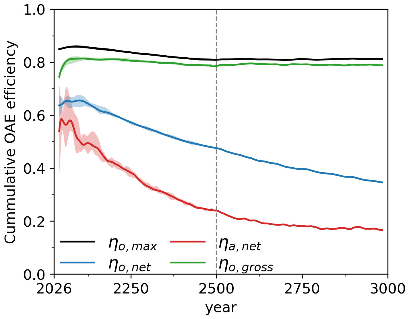
Figure 8 Cumulative efficiencies of ocean alkalinity enhancement; maximum ocean capture efficiency η_o,max in black, net ocean capture efficiency η_o,net in blue, net atmospheric CO₂-reduction η_a,net in red and gross ocean capture efficiency η_o,gross in green for 2 °C global warming stabilization simulations including the first ensemble member that has been extended until year 3000. All lines are ensemble and 31 year running means, while the shading represents the ensemble spread. OAE termination for the first ensemble member after 2500 is marked with the vertical dashed line.

Regional differences in maximum ocean capture efficiency at the surface reflect the sensitivity of surface pCO₂ to alkalinity relative to dissolved inorganic carbon, which is lowest in the tropics and highest at high latitudes (Fig. C5a). This is consistent with regional differences in the buffer capacity (Egleston et al., 2010). In some regions such as the North Atlantic, North Pacific and parts of the Southern Ocean, gross uptake efficiency locally exceeds the theoretical maximum expected from surface alkalinity addition alone (Fig. C5b). This is due to lateral redistribution of un-equilibrated alkalinity by ocean circulation, which adds local carbon uptake potential and explains the larger than maximum efficiency. Additionally, these regions exhibit higher gas transfer velocities (Zhou et al., 2023). Therefore, less un-equilibrated alkalinity is transported away from these regions, while incoming un-equilibrated alkalinity can equilibrate faster locally. However, Zhou et al. (2024) show no specifically high efficiency in these regions when alkalinity is only added within the region itself, and Burger et al. (2026) find a strongly increased efficiency in these regions due to resurfacing of alkalinity that was added below the surface in other regions, both indicating that the redistribution of un-equilibrated alkalinity is the dominant process.

3.4 Ocean acidification response

The addition of alkalinity leads to a pronounced increase in global mean ocean surface pH relative to the reference scenarios (Fig. 9a). In the absence of alkalinity enhancement (Reference scenarios), global mean surface pH initially declines and subsequently recovers during the global warming stabilization phase, reflecting the initial rise and later decline in atmospheric CO₂. In the OAE scenarios, global mean surface pH during the period 2470 to 2500 is elevated relative to the reference scenario by 0.105 [0.103–0.106] in the 1.5 °C scenario, 0.111 [0.109–0.112] in the 2 °C, and 0.124 [0.123–0.126] in the 3 °C scenario (Fig. 9b). Under the 1.5 °C scenario, this increase is sufficient to raise global mean surface pH above pre-industrial levels, thereby fully reversing historical surface ocean acidification. The temporal evolution of surface pH closely follows that of atmospheric CO₂, with the largest pH changes occurring in the high-warming scenario, where OAE leads to the strongest atmospheric CO₂ drawdown. This is also evident at the regional scale. All regions experience increases in surface pH due to OAE, with slightly larger changes in the 3 °C scenario compared to the lower warming scenarios (Fig. C2d–f).

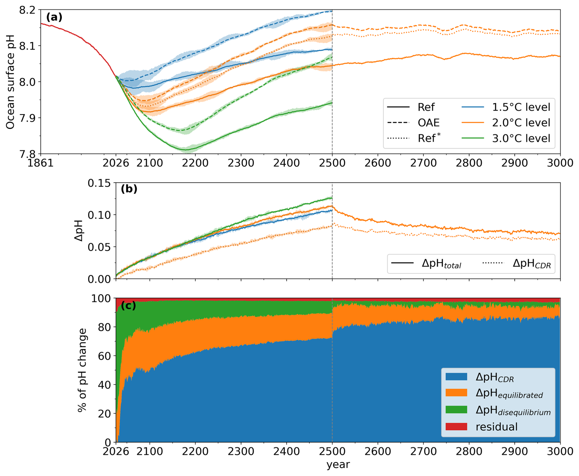
Figure 9 Global ocean surface pH in (a), global surface pH change due to OAE in (b) and contributions to the total global surface pH change due to OAE in (c). Panel (b) shows pH differences between OAE and reference simulations as well as the contribution of the CDR effect. Panel (c) shows the relative contributions from CDR, pH-equilibrated, pCO₂ disequilibrium and residual to the total pH change between OAE and the reference 2 °C simulation. In all panels ensemble means until 2500 are shown and then OAE termination in 2500 for one ensemble member in the 2 °C scenario. Shading in (a) and (b) indicates the ensemble range. Dashed vertical grey lines indicate the timing of OAE termination at year 2500.

The increase in global surface pH is primarily driven by the reduction in atmospheric CO₂, with smaller additional contributions from OAE-specific direct chemical effects, such as the equilibrated pH response and transient pCO₂ disequilibrium (Fig. 9c; see Sect. 2.4 for further details on the method). In 2100 in the 2 °C global warming scenario, the combined direct chemical effects of OAE account for about 48 % of the total additional pH increase. Over time, the ocean–atmosphere system progressively equilibrates, and the contribution from atmospheric CO₂ drawdown becomes increasingly dominant, while both direct chemical effects diminish. Averaged over 2470 to 2500, approximately 72 % of the total global surface pH increase can be attributed to reduced atmospheric CO₂, 17 % due to equilibrated pH response and 9 % due to remaining pCO₂ disequilibrium. The residual is a result of approximations in calculating the three contributions.

Following OAE termination in 2500, the pH difference between the OAE simulation and reference simulation gradually declines (Fig. 9b), resulting in a remaining pH response of 0.071 in the year 3000. This reduction in OA mitigation is initially dominated by a decrease in pCO₂ disequilibrium (Fig. 9c), as surface waters continue to equilibrate in the decades following termination. However, ongoing upwelling and mixing of previously subducted alkalinity continue to lower oceanic pCO₂, maintaining a nearly constant pCO₂ offset of around 2 µatm between the OAE and Ref^∗ simulations. Consequently, pCO₂ disequilibrium still explains 2 % of the total pH change 500 years after OAE termination. The contribution of the equilibrated pH response also decreases after 2500, reflecting the declining surface alkalinity difference between the OAE and reference simulations, and accounts for approximately 7 % of the pH response in the year 3000. In contrast, while the carbon dioxide removal effect weakens after OAE termination (Fig. 9b), its relative importance increases, explaining about 88 % of OA mitigation by the year 3000. This weakening of the CDR effect is due to continued outgassing of oceanic CO₂ after OAE termination, driving an increase in atmospheric CO₂ and a decrease in surface ocean pH.

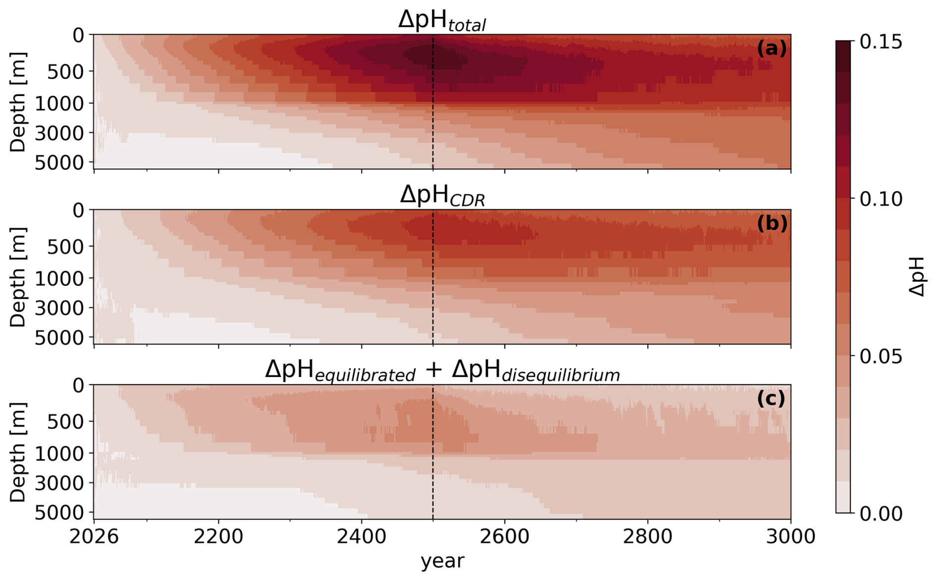
Figure 10 Hovmoeller plots of pH differences due to OAE over depth and time for the 2 °C scenario. The total pH change in (a), the pH response to CDR in (b) and the sum of the pH-equilibrated and pCO₂ disequilibrium effects in (c). All plots show the global horizontal averages, ensemble means until 2500 and the first ensemble member with OAE termination after 2500 (vertical dashed line). Note the irregular y-axis, with a break at 1000 m depth.

In the subsurface ocean, the largest global mean ocean acidification mitigation from OAE is simulated at a depth of around 250 m, with a maximum pH increase of 0.137 [0.135–0.139] by year 2500 in the 2 °C scenario (Fig. 10a). As at the surface, the subsurface pH mitigation response is larger in the 3 °C scenario and smaller in the 1.5 °C scenario (not shown). The subsurface maximum reflects the competing effects of two opposing vertical gradients: the OAE-induced alkalinity enhancement and associated DIC reduction weakens with depth, whereas the sensitivity of pH to changes in alkalinity and DIC increases with depth. Their combined effect yields a maximum pH response below the surface. Similar subsurface maxima have also been reported for historical ocean acidification (Fassbender et al., 2023; Müller and Gruber, 2024). Consistent with the surface response, the direct chemical effects of OAE (Fig. 10c) contribute substantially early on, while the CDR effect becomes increasingly dominant over time (Fig. 10b). In 2100, the CDR effect explains 54 % of the total interior pH change, with the direct chemical effects accounting for the remaining 46 %. By 2500, the CDR contribution increases to 69 %. After OAE termination in 2500, the total subsurface pH mitigation gradually declines and the relative contribution of the CDR effect increases to 74 % by the year 3000. Below 1000 m, however, pH mitigation continues to increase despite the OAE termination, because ongoing ocean ventilation progressively propagates the accumulated pH deficit into the deep ocean on multi-centennial timescales.

4 Discussion and conclusion

In this study, we assess the efficiency of ocean alkalinity enhancement (OAE), along with its associated climate response and potential to mitigate ocean acidification, under different global warming stabilization scenarios using an emission-driven, comprehensive Earth system model.

We find that the global mean surface temperature decreases approximately linearly with continued alkalinity addition, and that the cooling per unit alkalinity added is similar across the three global warming stabilization scenarios. A comparable near-linear temperature response has also been reported by Martin et al. (2025). This suggests that a given amount of alkalinity produces roughly the same cooling effect under both low- and high-warming conditions. Because cumulative CO₂ removal also increases nearly linearly over time, due to an approximately constant, scenario-independent gross ocean capture efficiency, our results imply an approximately linear transient climate response to removal (TCRR) over the range of warming levels explored here (Fig. C6) (Matthews et al., 2009; Zickfeld et al., 2021; Evans and Matthews, 2025). This means that OAE-induced CO₂ removal, diagnosed from gross ocean carbon capture, can be readily incorporated into the well-established TCRE-based framework for estimating remaining carbon budgets consistent with specific temperature targets (Rogelj et al., 2019; Matthews et al., 2020). The near-linearity of the temperature response also indicates that, for OAE, a CDR-tax framework (Boyd et al., 2025b) to capture strong state-dependent changes in effectiveness may not be necessary, since the temperature response per unit addition of alkalinity remains approximately constant across the warming levels considered. Nevertheless, the robustness of this result remains to be tested across other Earth system models and experimental setups, such as carbon and/or temperature overshoot scenarios.

The definition of OAE efficiency strongly influences both its interpretation and policy relevance, as different metrics capture distinct aspects of ocean alkalinity enhancement. The maximum ocean capture efficiency varies between 0.81 and 0.86 when defined at the surface. These moderate variations follow changes in ocean buffer capacity along emission pathways and across global warming scenarios. The gross ocean capture efficiency (about 0.78–0.79 for the 2 °C scenario) quantifies the additional carbon uptake directly induced by OAE and thus reflects its negative emissions potential, making it well suited for carbon accounting and comparison with other CDR approaches such as direct air capture (Tyka, 2025). Similar to the maximum ocean capture efficiency, this metric is also relatively insensitive to the emission pathway. In contrast, the net ocean capture efficiency accounts for Earth system feedbacks that reduce net ocean carbon uptake following atmospheric CO₂ drawdown (Schwinger et al., 2024) and is highly dependent on the climate state. The net atmospheric CO₂ reduction efficiency is further reduced by the CO₂ efflux from the land carbon reservoir and is therefore lower than the net ocean capture efficiency. While the gross efficiency is most appropriate for policy and carbon accounting frameworks, net efficiencies remain essential for assessing long-term carbon storage and climate impacts, such as ocean acidification. Biogeochemical feedbacks in the ocean, such as due to state-dependent calcification rates, affect both gross and net ocean capture efficiencies, consistent with previous studies (Bednaršek et al., 2025; Lehmann and Bach, 2025). Overall, these feedbacks substantially lower the total additional alkalinity in the ocean, where a quite equal part of the reduction comes from chemical changes due to OAE or is related to the reduction in atmospheric CO₂ following OAE (see the difference of OAE and Ref^∗ to Ref in Fig. C3c). These feedbacks are relevant for ocean-only simulations as well, where estimates of gross efficiency can differ depending on whether they are defined as the change in oceanic DIC inventory relative to the change in alkalinity inventory or as the change in air–sea CO₂ flux relative to the added alkalinity, the latter representing negative emissions. In the ESM2M model, the inventory-based efficiency is higher than the flux-based efficiency (Fig. C7) due to enhanced calcification following increasing calcite and aragonite saturation states under the OAE addition. In 2500, inventory-based and flux-based efficiency differ by 0.01 units with distinct ensemble ranges. Furthermore, the inventory-based efficiency eventually surpasses the maximum ocean capture efficiency calculated at the surface and the full potential of OAE on timescales of millennia is rather limited by the mean ocean maximum efficiency, which is larger with about 0.91. We therefore emphasize that it is essential to clearly specify how efficiencies are calculated and which processes are represented in the applied model, as these choices directly affect policy-relevant efficiency estimates and associated uncertainties.

We show that OAE can mitigate ocean acidification. While surface ocean acidification already reverses in the global warming stabilization scenarios without OAE due to a long-term decline in atmospheric CO₂, OAE provides additional mitigation. In response to OAE, global mean pH increases by 0.11 to 0.12 (1.5 °C scenario to 3 °C scenario) at the surface and by up to 0.13 to 0.15 at subsurface. The majority of this pH increase is driven by the reduction in atmospheric CO₂, a response that is largely independent of the specific CDR approach. In addition, OAE induces direct chemical changes to the ocean carbonate system, which account for 48 % of the surface pH increase after 75 years of OAE and still contribute 27 % by the year 2500. Following termination of OAE, these OAE-specific effects diminish over time as the ocean–atmosphere system equilibrates and 88 % of surface pH mitigation in the year 3000 comes from reduced atmospheric CO₂. This indicates that emissions reductions remain the most effective and durable strategy for limiting ongoing ocean acidification, and that the long-term acidification mitigation potential provided by OAE is not substantially larger than that achieved through any other CDR approach that lowers atmospheric CO₂, at least on multi-centennial timescales. Although sustained alkalinity addition could, in principle, reduce peak ocean acidification, the required amounts of alkalinity would be immense. At regional and local scales, OAE has the potential to temporarily offset ocean acidification (Albright et al., 2016; Feng et al., 2016; Mongin et al., 2021). However, elevated pH levels, rapid pH changes or the addition of toxic trace metals through impure minerals may also have ecological impacts that remain poorly understood, underscoring the need for caution in deployment and further investigation of biological responses (Feng et al., 2016; Bednaršek et al., 2025; van de Mortel et al., 2025).

Although we consider our conclusions robust, several important caveats must be acknowledged. These relate primarily to (i) the magnitude, spatial distribution, and temporal characteristics of alkalinity deployment, (ii) assumptions regarding the dissolution of added minerals, and (iii) limitations arising from model resolution and simulated biogeochemical complexity. First, the representation of alkalinity addition in our simulations is highly idealized. The total amount of alkalinity applied far exceeds what could be realistically implemented in the near future (Eisaman et al., 2023), as the amount of needed materials, dependent on the feedstock, corresponds to or exceeds the current scale of global production (Renforth and Henderson, 2017; Martin et al., 2025), along with substantial infrastructure requiring large investments. Another important point for the readiness of OAE are life cycle emissions, which need emission reductions themselves to make the approach net carbon negative (Foteinis et al., 2022; Delval et al., 2025). Moreover, our simulations assume near global deployment, whereas real-world application would likely be spatially constrained to exclusive economic zones, coastal regions, or shipping corridors (Lezaun, 2021; He and Tyka, 2023). We further assume continuous alkalinity addition, while practical deployment can occur in temporally discrete pulses as well. Continuous addition is likely feasible at specific coastal sites, such as industrial water outlets (Wang et al., 2023; Burt et al., 2024) and continuous alkalinity addition may well approximate the alkalinity release from frequent individual pulses necessary for OAE at scale. Second, we assume instantaneous dissolution of the added minerals at the ocean surface. Depending on the mineral and grain size, however, dissolution kinetics and particle sinking can substantially delay alkalinity release and reduce near-term carbon uptake efficiency (Köhler et al., 2013; Fakhraee et al., 2023; Burger et al., 2026). More realistic representations of mineral dissolution and particle dynamics are therefore required to better constrain OAE efficiency under plausible deployment scenarios. Third, despite a comparatively realistic representation of alkalinity relative to other Earth system models (Planchat et al., 2023), including explicit aragonite and calcite cycling, several model limitations may influence the simulated OAE response. Notably, the biogeochemical module lacks a more explicit representation of the biological carbon pump, such as particulate organic carbon dynamics, and more detailed sediment-water interactions, both of which could affect long-term carbon and alkalinity cycling. The model also exhibits regional alkalinity biases that may limit its applicability for assessing geographically specific OAE deployments (Dunne et al., 2013). Furthermore, the coarse ocean resolution restricts the representations of mesoscale processes, particularly in western boundary current regions, where we identify strong carbon uptake responses (Guo and Timmermans, 2024). While higher spatial resolution and increased biogeochemical complexity would improve process fidelity, such fully coupled simulations remain computationally prohibitive for the ensemble, multi-centennial simulations across multiple emission scenarios conducted here.

In summary, we demonstrate that the net ocean carbon uptake and the resulting atmospheric CO₂ reduction from OAE are modulated by global carbon cycle feedbacks that vary with the emission trajectory. In contrast, the simulated cooling evolves approximately linearly over time, consistent with a near-constant transient climate response to removal (TCRR) under sustained CO₂ drawdown. On centennial timescales, OAE mitigates ocean acidification primarily through reduced atmospheric CO₂; an effect common to other CDR approaches. Direct chemical pH increase from added alkalinity is most important during the first decades and becomes progressively less important thereafter. Overall, these results underscore that rapid emission reductions remain the most effective strategy for achieving the Paris Agreement goals and mitigating ocean acidification.

Appendix A: Equivalence of OAE and direct air capture in reducing atmospheric CO₂

We investigate whether OAE in an emission-driven framework leads to the same reduction in atmospheric CO₂ as would be obtained by applying the additional ocean carbon uptake diagnosed from a concentration-driven OAE simulation as negative emissions in an emission driven simulation (i.e. equivalent to direct air capture (DAC)). This analysis reassesses the findings of Tyka (2025) using a fully coupled Earth system model. The additional carbon uptake is equivalent to the gross ocean carbon capture, which is also quantified by the gross ocean capture efficiency.

To test this, we performed a set of 200 years pre-industrial simulations (Fig. A1): (i) an emission-driven control simulation with zero emissions (red line), (ii) a concentration-driven simulation with atmospheric CO₂ fixed at 286 ppm and no OAE (orange line), (iii) a concentration-driven simulation with atmospheric CO₂ fixed at 286 ppm and continuous OAE applied using the same forcing as described in Sect. 2.2 (blue line), (iv) an emission-driven simulation in which the difference in ocean carbon uptake between simulations (ii) and (iii) is imposed as a negative emission forcing, directly removing carbon from the atmospheric reservoir and the global carbon cycle can react to the changes in atmospheric CO₂ (purple line), and (v) an emission-driven simulation with zero emissions, but with OAE applied identically to simulation (iii) (green line).

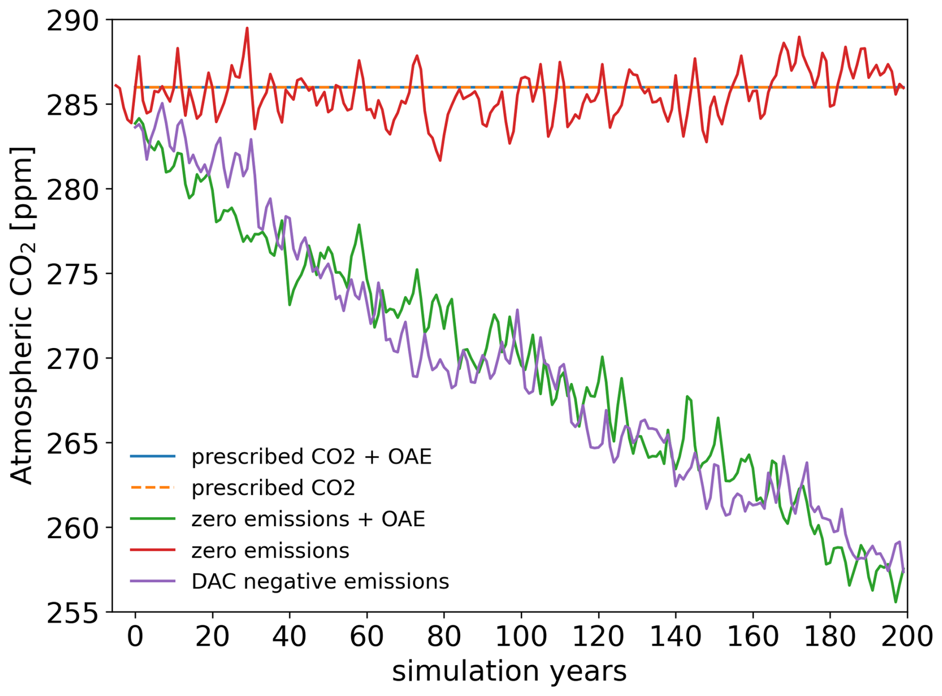
Figure A1 Simulated atmospheric CO₂ concentrations in a set of pre-industrial simulations. Details are explained in Appendix A.

The emission-driven simulations with negative emissions (purple) and with OAE (green) exhibit nearly identical reductions in atmospheric CO₂ supporting the findings of Tyka (2025). The small difference may be explained by internal variability, which is on the same order as in the control (red). This result demonstrates that carbon cycle feedbacks respond equivalently to CO₂ removal from the atmosphere and to additional ocean carbon uptake induced by OAE. Therefore, concentration-driven ocean-only model simulations with and without OAE are sufficient to quantify the expected carbon removal from OAE, hence the gross ocean capture efficiency, and to inform carbon accounting and crediting frameworks (Tyka, 2025). Fully coupled Earth system models, however, remain essential for assessing the broader climate response.

Appendix B: Derivation of the pH-equilibrated effect

The ocean carbonate system is governed by the equilibrium constants relating oceanic partial pressure of CO₂ (pCO₂), carbonic acid ($\left[{\mathrm{H}}_{\mathrm{2}}{\mathrm{CO}}_{\mathrm{3}}^{\ast }\right]$), bicarbonate ($\left[{\mathrm{HCO}}_{\mathrm{3}}^{-}\right]$), carbonate ions ($\left[{\mathrm{CO}}_{\mathrm{3}}^{\mathrm{2}-}\right]$), and protons ([H⁺]):

$$K_{\mathrm{0}}={\displaystyle \frac{\left[{\mathrm{H}}_{\mathrm{2}}{\mathrm{CO}}_{\mathrm{3}}^{\ast }\right]}{p{\mathrm{CO}}_{\mathrm{2}}}},K_{\mathrm{1}}={\displaystyle \frac{\left[{\mathrm{H}}^{+}\right]\left[{\mathrm{HCO}}_{\mathrm{3}}^{-}\right]}{\left[{\mathrm{H}}_{\mathrm{2}}{\mathrm{CO}}_{\mathrm{3}}^{\ast }\right]}},K_{\mathrm{2}}={\displaystyle \frac{\left[{\mathrm{H}}^{+}\right]\left[{\mathrm{CO}}_{\mathrm{3}}^{\mathrm{2}-}\right]}{\left[{\mathrm{HCO}}_{\mathrm{3}}^{-}\right]}}.$$

Combining these expressions yields two equivalent formulations for pCO₂:

$$p{\mathrm{CO}}_{\mathrm{2}}={\displaystyle \frac{\left[{\mathrm{H}}^{+}\right]\left[{\mathrm{HCO}}_{\mathrm{3}}^{-}\right]}{K_{\mathrm{0}}{K}_{\mathrm{1}}}}\text{ and }p{\mathrm{CO}}_{\mathrm{2}}={\displaystyle \frac{\left[{\mathrm{H}}^{+}{]}^{\mathrm{2}}\right[{\mathrm{CO}}_{\mathrm{3}}^{\mathrm{2}-}]}{K_{\mathrm{0}}{K}_{\mathrm{1}}{K}_{\mathrm{2}}}}.$$

We assume that alkalinity addition induces a change in pCO₂ that fully equilibrates with the atmosphere, such that the pCO₂ remains unchanged before and after equilibration:

$$\begin{array}{}\text{(B1)}& {p{\mathrm{CO}}_{\mathrm{2}}}^{\text{start}}={p{\mathrm{CO}}_{\mathrm{2}}}^{\text{end}}.\end{array}$$

This implies

$$\begin{array}{}\text{(B2)}& {\left[{\mathrm{H}}^{+}\right]}^{\text{start}}{\left[{\mathrm{HCO}}_{\mathrm{3}}^{-}\right]}^{\text{start}}={\left[{\mathrm{H}}^{+}\right]}^{\text{end}}{\left[{\mathrm{HCO}}_{\mathrm{3}}^{-}\right]}^{\text{end}}\end{array}$$

and

$$\begin{array}{}\text{(B3)}& ({\left[{\mathrm{H}}^{+}\right]}^{\text{start}}{)}^{\mathrm{2}}{\left[{\mathrm{CO}}_{\mathrm{3}}^{\mathrm{2}-}\right]}^{\text{start}}=({\left[{\mathrm{H}}^{+}\right]}^{\text{end}}{)}^{\mathrm{2}}{\left[{\mathrm{CO}}_{\mathrm{3}}^{\mathrm{2}-}\right]}^{\text{end}}.\end{array}$$

Uptake of atmospheric CO₂ by the ocean predominantly increases the bicarbonate concentration ($\left[{\mathrm{HCO}}_{\mathrm{3}}^{-}\right]$) (Orr et al., 2005). We therefore introduce a small parameter ϵ≪1 describing the relative increase in bicarbonate during equilibration:

$$\begin{array}{}\text{(B4)}& {\displaystyle \frac{{\left[{\mathrm{HCO}}_{\mathrm{3}}^{-}\right]}^{\text{end}}}{{\left[{\mathrm{HCO}}_{\mathrm{3}}^{-}\right]}^{\text{start}}}}=\mathrm{1}+\mathit{ϵ}.\end{array}$$

Combining Eqs. (B2)–(B4) yields:

$$\begin{array}{}\text{(B5)}& {\displaystyle \frac{{\left[{\mathrm{CO}}_{\mathrm{3}}^{\mathrm{2}-}\right]}^{\text{end}}}{{\left[{\mathrm{CO}}_{\mathrm{3}}^{\mathrm{2}-}\right]}^{\text{start}}}}=(\mathrm{1}+\mathit{ϵ}{)}^{\mathrm{2}}.\end{array}$$

The total change in dissolved inorganic carbon (ΔDIC) due to OAE is given by the change in bicarbonate and carbonate concentrations:

$$\begin{array}{}\text{(B6)}& \begin{array}{rl}\mathrm{\Delta }\text{DIC}=& {\left[{\mathrm{HCO}}_{\mathrm{3}}^{-}\right]}^{\text{end}}+{\left[{\mathrm{CO}}_{\mathrm{3}}^{\mathrm{2}-}\right]}^{\text{end}}-{\left[{\mathrm{HCO}}_{\mathrm{3}}^{-}\right]}^{\text{start}}\\ & -{\left[{\mathrm{CO}}_{\mathrm{3}}^{\mathrm{2}-}\right]}^{\text{start}}.\end{array}\end{array}$$

By using Eqs. (B4) and (B5), this yields:

$$\begin{array}{}\text{(B7)}& \mathrm{\Delta }\text{DIC}=\mathit{ϵ}{\left[{\mathrm{HCO}}_{\mathrm{3}}^{-}\right]}^{\text{start}}+(\mathrm{2}\mathit{ϵ}+{\mathit{ϵ}}^{\mathrm{2}}){\left[{\mathrm{CO}}_{\mathrm{3}}^{\mathrm{2}-}\right]}^{\text{start}}.\end{array}$$

Since ΔDIC is positive for OAE, ϵ is positive as well and assuming that ϵ²≈0 since ϵ≪1, this simplifies to

$$\begin{array}{}\text{(B8)}& \mathrm{\Delta }\text{DIC}=\mathit{ϵ}\left({\left[{\mathrm{HCO}}_{\mathrm{3}}^{-}\right]}^{\text{start}}+\mathrm{2}{\left[{\mathrm{CO}}_{\mathrm{3}}^{\mathrm{2}-}\right]}^{\text{start}}\right).\end{array}$$

The bracket in Eq. (B8) describes the contribution of bicarbonate and carbonate ions to alkalinity. As bicarbonate and carbonate ions makes up about 96 % of the alkalinity in the ocean (Sarmiento and Gruber, 2006), we assume this to be the total alkalinity of the ocean before alkalinity addition, i.e. the alkalinity in the reference simulation (ALK^Ref). Equation (B8) can therefore be written as:

$$\begin{array}{}\text{(B9)}& \mathrm{\Delta }\text{DIC}=\mathit{ϵ}{\mathrm{ALK}}^{\mathrm{Ref}}.\end{array}$$

As discussed in Sect. 2.3.3, under perfect equilibration, the total additional DIC change is proportional to the added alkalinity, with the proportionality given by the maximum ocean capture efficiency η_o,max:

$$\begin{array}{}\text{(B10)}& \mathrm{\Delta }\text{DIC}={\mathit{\eta }}_{\mathrm{o},\text{max}}\mathrm{\Delta }\text{ALK}.\end{array}$$

Using Eqs. (B9) and (B10), we can write ϵ as:

$$\begin{array}{}\text{(B11)}& \mathit{ϵ}={\mathit{\eta }}_{\mathrm{o},\text{max}}{\displaystyle \frac{\mathrm{\Delta }\text{ALK}}{{\mathrm{ALK}}^{\mathrm{Ref}}}}.\end{array}$$

To quantify the pH after equilibration, we combine Eqs. (B2) and (B4) and get the amount of protons after equilibration:

$$\begin{array}{}\text{(B12)}& {\left[{\mathrm{H}}^{+}\right]}^{\text{end}}={\displaystyle \frac{\mathrm{1}}{\mathrm{1}+\mathit{ϵ}}}{\left[{\mathrm{H}}^{+}\right]}^{\text{start}}.\end{array}$$

And since $\text{pH}=-{\text{log}}_{\mathrm{10}}\left(\left[{\mathrm{H}}^{+}\right]\right)$, the pH after equilibration can be calculated as:

$$\begin{array}{}\text{(B13)}& {\text{pH}}^{\text{end}}={\text{log}}_{\mathrm{10}}(\mathrm{1}+\mathit{ϵ})+{\text{pH}}^{\text{start}}.\end{array}$$

Since ϵ≪1, we can approximate ${\text{log}}_{\mathrm{10}}(\mathrm{1}+\mathit{ϵ})\approx \mathit{ϵ}\frac{\mathrm{1}}{\ln \left(\mathrm{10}\right)}$, and the pH-equilibrated effect is approximated by:

$$\begin{array}{}\text{(B14)}& \begin{array}{rl}\mathrm{\Delta }{\text{pH}}_{\text{equilibrated}}& ={\text{pH}}^{\text{end}}-{\text{pH}}^{\text{start}}\\ & ={\mathit{\eta }}_{\mathrm{o},\text{max}}{\displaystyle \frac{\mathrm{\Delta }\text{ALK}}{{\mathrm{ALK}}^{\mathrm{Ref}}}}{\displaystyle \frac{\mathrm{1}}{\ln \left(\mathrm{10}\right)}}\end{array}\end{array}$$

Appendix C: Additional Figures

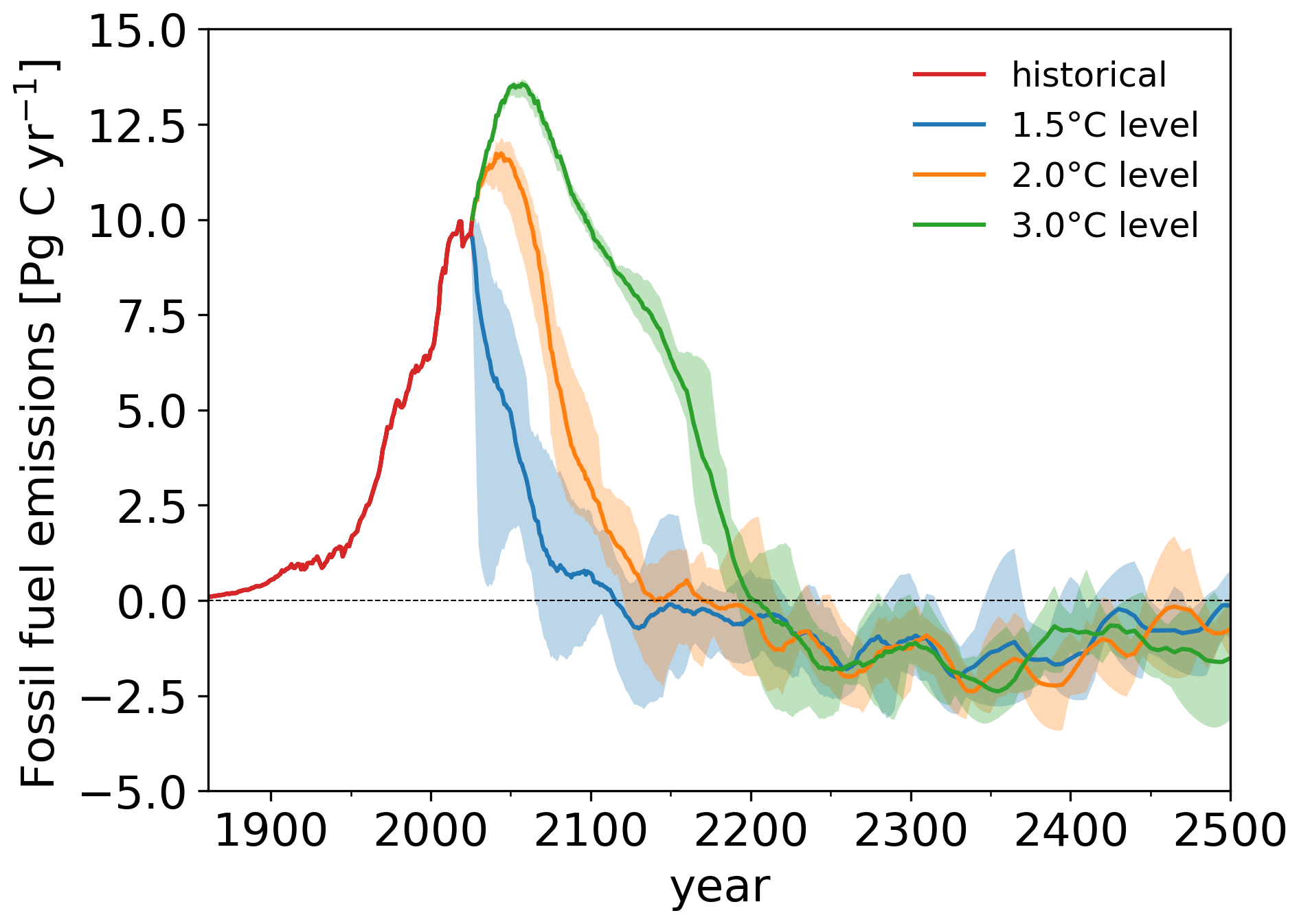
Figure C1 Emission trajectories from the adaptive emission reduction approach to stabilise at global warming levels of 1.5, 2.0 and 3.0 °C. All lines are ensemble means, while the shading represents the ensemble range.

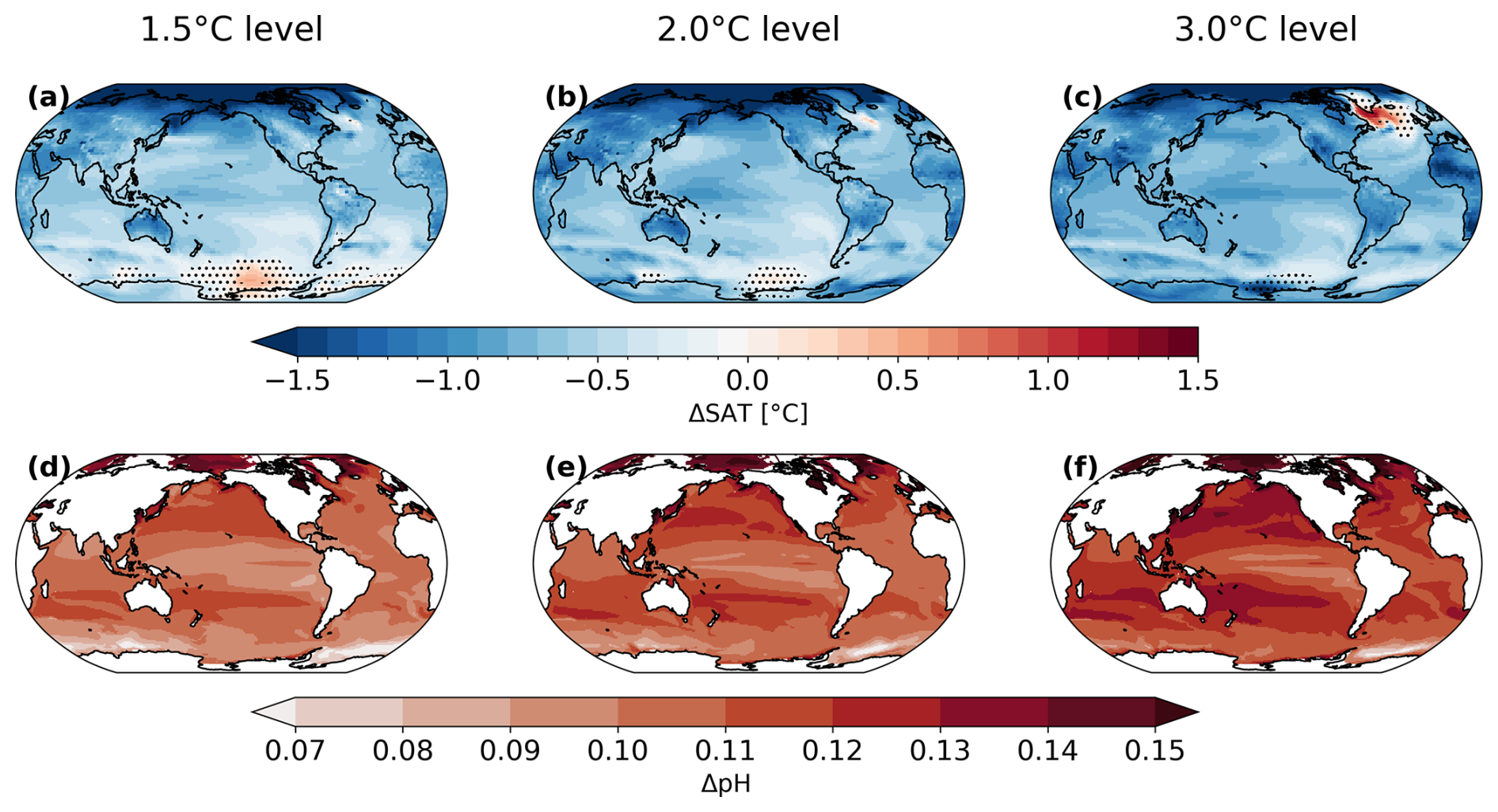
Figure C2 Regional patterns of surface air temperature (a–c) and surface pH (d–f) changes between the OAE and the reference simulation for the period of 2470–2500 for the 1.5 °C level (a, d), the 2 °C level (b, e) and the 3 °C level (c, f). Regions without hatching show significance at the 95 % level based on a two-sided students t-test.

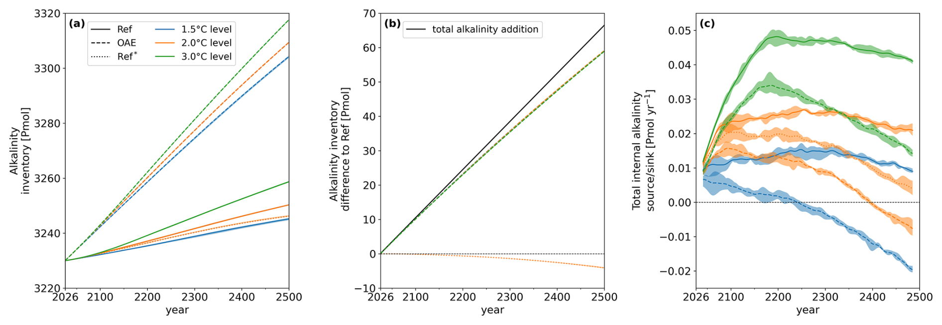
Figure C3 Simulated ocean alkalinity inventories (a), differences in the alkalinity inventory of the OAE and Ref^∗ simulations to the Ref simulation (b) and the sum of all ocean internal alkalinity sources and sinks, including sediment processes (c) for all global warming scenarios with and without OAE. Lines are the 5 member ensemble mean and shading refers to the ensemble range. Lines in panel (c) are smoothed with a 31 year running mean.

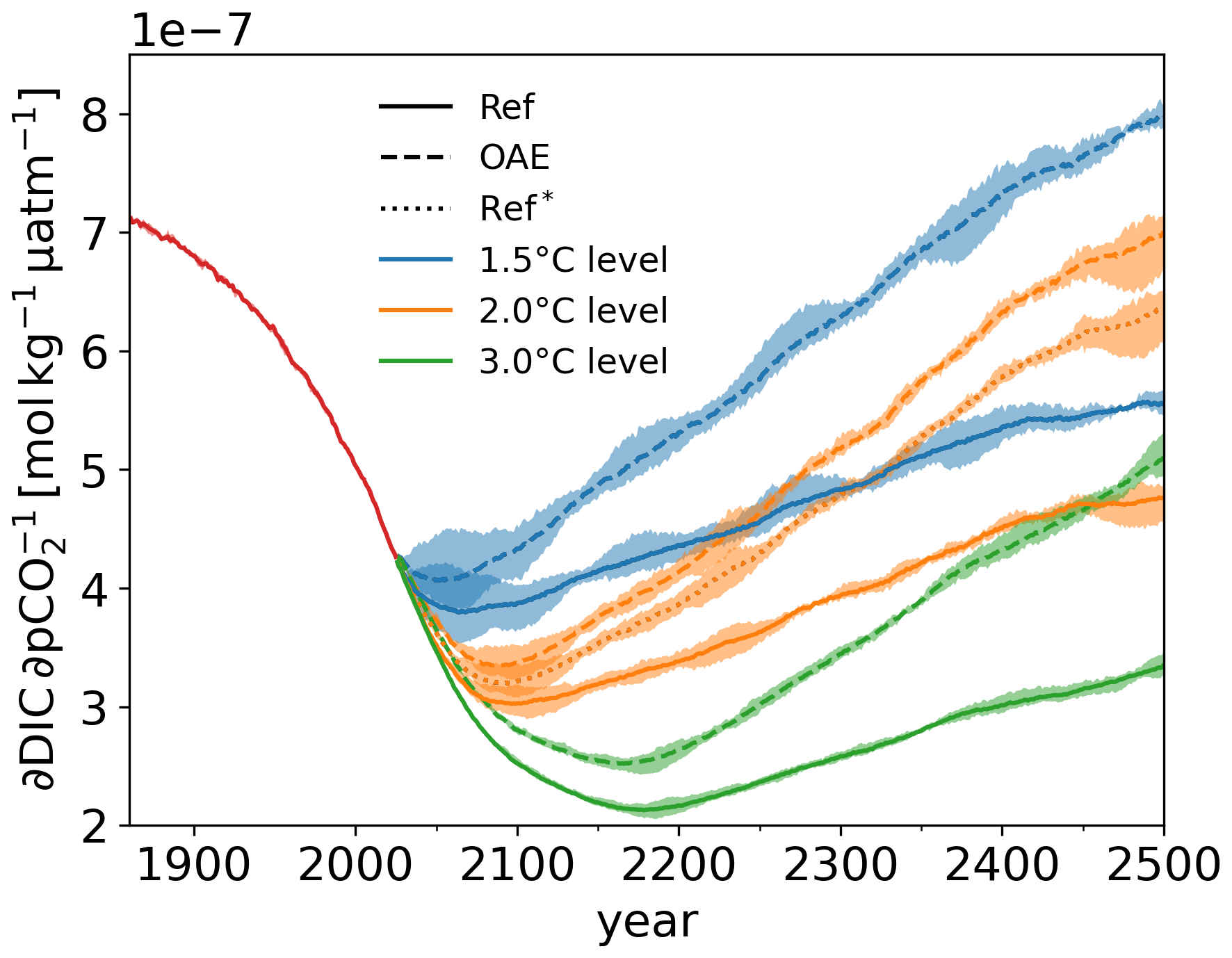
Figure C4 The global ocean buffer capacity from 1861 until 2500 for the different global warming scenarios with and without OAE. Lines are the 5 member ensemble mean and shading refers to the ensemble range. A low buffer capacity represents a high sensitivity of pCO₂ to DIC and a high Revelle factor and vice versa (Revelle and Suess, 1957).

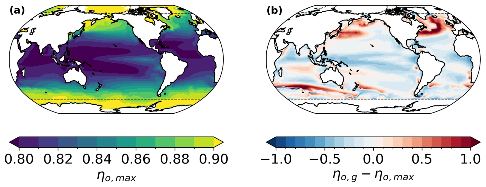
Figure C5 Spatial pattern of the maximum ocean capture efficiency (a) and the difference between the gross ocean capture efficiency and the maximum ocean capture efficiency (b), averaged over 2026 and 2500.

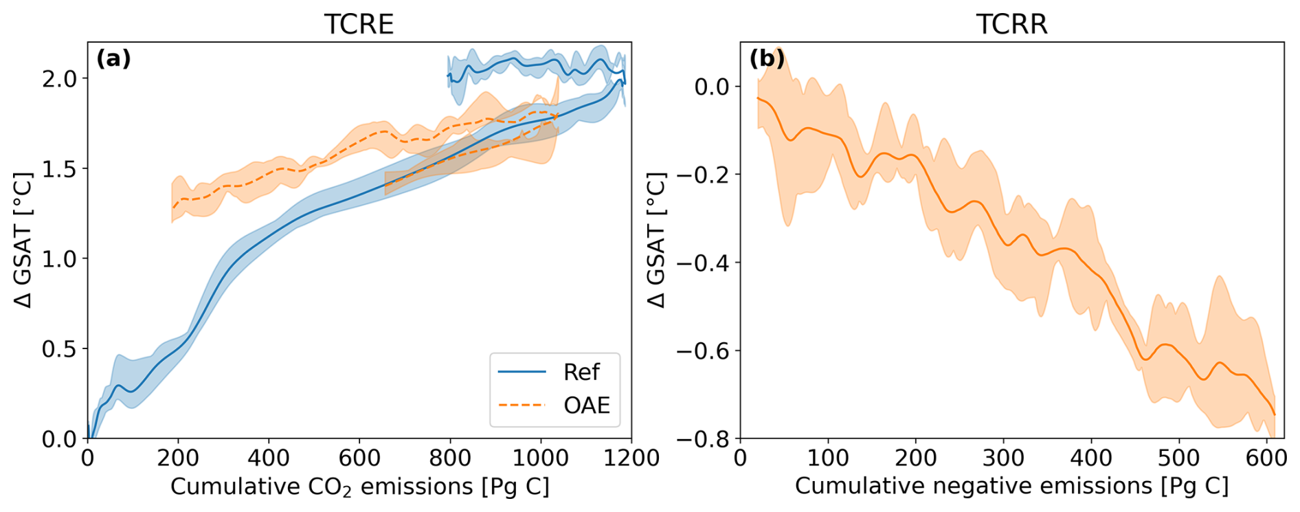
Figure C6 Simulated transient climate response to cumulative CO₂ emissions (TCRE) in (a) and transient climate response to removal (TCRR) in (b). Panel (a) show TCRE for the reference simulation (Ref) and the global surface air temperature response to the total positive fossil fuel emissions plus negative emissions due to OAE (OAE). Panel (b) shows the TCRR as the temperature difference between OAE and the reference simulation against the cumulative negative CO₂ emissions resulting from the gross carbon capture efficiency. The figure only shows the 2 °C scenario, since the Ref^∗ simulations are necessary to calculate negative emissions. All lines are ensemble and 31 year running means, while the shading represents the ensemble spread.

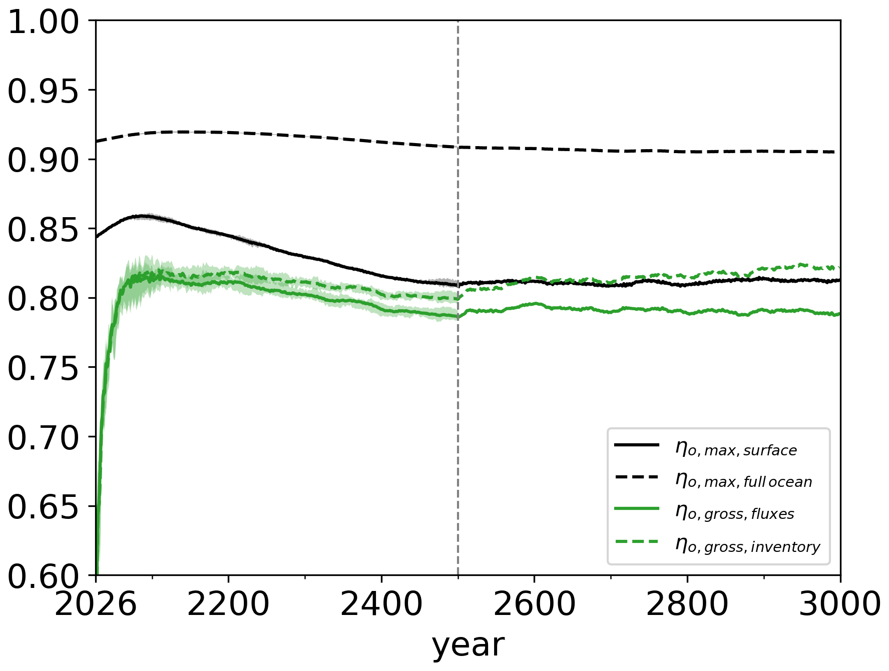
Figure C7 Cumulative efficiencies of ocean alkalinity enhancement; maximum ocean capture efficiency η_o,max in black and gross ocean capture efficiency η_o,gross in green for the 2 °C global warming scenario. Surface maximum efficiency and gross efficiency from air–sea CO₂ fluxes in the solid lines, average maximum efficiency for the full ocean and gross efficiencies from DIC and alkalinity inventory changes in the dashed lines. All lines are ensemble means, while the shading represents the ensemble spread. OAE termination for the first ensemble member after 2500 is marked with the vertical dashed line.