Combined water table and temperature dynamics control CO₂ emission estimates from drained peatlands under rewetting and climate change scenarios

This study integrates process-based hydrological modeling and empirical CO₂ flux modeling at a daily temporal resolution to evaluate how peatland hydrology influence CO₂ emissions under scenarios of rewetting and climate change.

Following the calibration of a three-dimensional transient physically-based hydrological model for a peat-dominated catchment, daily groundwater table dynamics were simulated to represent hydrological conditions in drained peat soils. These simulations were coupled with an empirical CO₂ flux model, developed from a comprehensive daily dataset of groundwater table depth, temperature, and soil CO₂ flux measurements. The empirical CO₂ flux model captures a clear temperature-dependent response of soil CO₂ emissions to variations in groundwater table depth.

By applying this coupled modeling framework, we quantified CO₂ emissions at daily timescales. The results demonstrate that incorporating both temperature sensitivity and high-resolution temporal variability in water level significantly influences projections of CO₂ fluxes. Especially the co-occurrence of elevated air temperature and low groundwater table significantly influence CO₂ emissions under scenarios of rewetting and climate change. These insights highlight the importance of including changing climate conditions in future peatland management strategies for emission inventories.

The study illustrates the value of combining detailed hydrological simulations with emission models. It also emphasizes the need for detailed monitoring of greenhouse gas emissions across multiple sites and the development of robust empirical models that can be generalized and spatially upscaled.

1 Introduction

Drained peatlands are widely accepted as being net greenhouse gas (GHG) sources and rewetting of peatlands is considered an effective means of overall net GHG emission reduction (Leifeld et al., 2019). The depth of the groundwater table below the surface i.e. the water table depth (WTD) largely controls the annual emissions of carbon dioxide (CO₂) and methane (CH₄) from organic soils, where deeper WTD results in CO₂ emissions and a shallow WTD increases CH₄ emissions (Evans et al., 2021). Despite triggering CH₄ emissions, rewetting of organic soils will still lead to a net long-term reduction of GHG emissions (Günther et al., 2020). However, current estimates of GHG emissions from drained and rewetted peatlands are still quite uncertain due to a lack of long-term monitoring and simplified modeling approaches.

Commonly adopted methodologies for estimating contribution of organic soils in national GHG inventories (Arents et al., 2018; Evans et al., 2021; Koch et al., 2023; Tiemeyer et al., 2020) are based on empirical response functions between long-term annual mean WTD estimates from data-driven machine learning (ML) models (Bechtold et al., 2014; Koch et al., 2023) and observed net ecosystem GHG budgets (Tiemeyer et al., 2020). Those methodologies allow regional upscaling and integration into national emission estimates.

However, significant variability in the observed net ecosystem carbon balance (NECB) used to derive the empirical relationship can be attributed to site-specific factors, including intra-annual (seasonal) WTD and temperature dynamics (Tiemeyer et al., 2020) caused by fluctuating climate. The current GHG inventory methods are not suited to account for extremes such as drought and flooding that have a profound, but temporally limited (days, weeks or months) impact on WTD. Especially the frequency and severity of droughts can have major impacts on the CO₂ emissions as WTD increases together with temperature (Olefeldt et al., 2017). Therefore, temperature changes also directly impact GHG emissions, as soil CO₂ and CH₄ production are temperature sensitive. Currently, the impact of short-term compound events e.g., simultaneous warm and dry conditions on annual CO₂ emissions from peat soil is little known (Zscheischler et al., 2020). Such events can lead to consequences like a deep groundwater table, highlighting the need for improved understanding of how climate variability and long-term change (Olefeldt et al., 2017) affect future CO₂ emissions from both drained and rewetted peatlands.

For Denmark, it is generally expected that, as a result of climatic changes, annual mean WTD will decrease (water tables closer to surface). However, this decrease in annual mean WTD is primarily attributed to a decrease in WTD during the wetter winter months, while warmer future summers are anticipated to experience minimal decrease or even increase in summer WTD (water tables deeper below the surface) and more prolonged periods with increased WTD (Henriksen et al., 2023; Seidenfaden et al., 2022).

The ML and statistical models of annual mean WTD (Bechtold et al., 2014; Koch et al., 2023) utilized in current national GHG inventories (Gyldenkærne et al., 2025; Koch et al., 2023; Nielsen et al., 2025; Tiemeyer et al., 2020) effectively reflect the spatial variability at the national scale, but most current ML WTD models are temporally invariant and account for neither inter-annual (between-year) variability nor seasonal or intra-annual variability in WTD or temperature. To establish WTD-CO₂ relations at intra-annual time scales, capable of capturing the impact of short-lived extreme events such as droughts and inundations, WTD time series at these finer temporal resolutions are required. For this, process-based transient 3D hydrological models capable of integrating unsaturated-saturated flow models to predict spatial and temporal variability of WTD are highly useful. Combined with the WTD-CO₂ relation we claim these model outputs can be used to calculate the CO₂ emissions on daily, seasonal, and inter-annual timescales.

Such hydrological models provide the potential for improving our estimation of peatland hydrology and thereby the spatio-temporal WTD variability. Improved representation of temporal variability of WTD are needed for refining the current and future GHG estimates that cannot be derived using the simple application of IPCC default emission factors (IPCC, 2014). Process-based hydrological models offer the opportunity to assess the effect of different management strategies and environmental conditions, such as rewetting and climate change.

Process-based hydrological models are increasingly being applied to study dynamics of peatland hydrology (Mozafari et al., 2023). For instance, Land Surface Models (LSM) (Bechtold et al., 2019; Largeron et al., 2018; Shi et al., 2015; Yuan et al., 2021) are employed to analyze the soil–plant–atmosphere exchange processes of water, energy and carbon. However, most LSMs rely on a simplified conceptual representation of hydrologic processes and are characterized by coarse spatial scales.

Of the studies applying fully integrated unsaturated-saturated flow models for peatland hydrology, some focus on site or field-scale models (Friedrich et al., 2023; Haahti et al., 2015; Java et al., 2021; Stenberg et al., 2018) while others apply the models at catchment scale (Ala-aho et al., 2017; Duranel et al., 2021; Friedrich et al., 2023; Jutebring et al., 2018; Lewis et al., 2013). A catchment scale approach with water balance closure is particularly important for climate change impact predictions, since the boundary conditions to the peatlands will also be affected by climate change. Similarly, the use of catchment scale models is important because impact evaluations of peatland management scenarios, such as rewetting, can also include impacts on streamflow and groundwater levels in neighboring areas.

The objectives of this study were to (1) estimate current and predict the future hydrology and soil CO₂ emissions in a Northern European drained peatland and (2) investigate the role of rewetting and climatic extremes on annual CO₂ emissions. To achieve these objectives, we used a transient physically-based hydrological 3D model to predict daily WTD for a case study area, the Tuse Stream catchment, representing a typical degraded Danish peatland. Secondly, we developed an empirical soil CO₂ flux (fCO₂) model based on coupled CO₂ flux, WTD and temperature observations for a similar Danish peatland (Nielsen et al., 2026), capable of making daily predictions. Combining the mechanistic hydrological model and the empirical emission model enabled the estimation of daily soil CO₂ fluxes under current conditions as well as scenarios of rewetting and future climate, while accounting for the impact of climatic variability and extremes.

2 Data and methodology

2.1 Study area

Tuse Stream catchment is located on the island of Zealand in the eastern part of Denmark (Fig. 1a). The total area encompasses 107 km² of which 19 km² are peat soil. The areal extent of peat soil was determined using a national map of organic soils (Adhikari et al., 2014). The largest continuous peat area within the catchment is a 13 km² drained fen located in a river valley (Fig. 1c) in the low-lying part of the catchment. The peat soil area is primarily used for agriculture. In small parts of the area, the drainage has been stopped to restore the natural hydrologic regime. The measured peat layer thickness extends from 0.4 to 3.5 m, below which alluvial sand deposits are typically found. Generally, the deeper geology in the area can be characterized as clay-dominated glacial till deposits. The catchment is characterized by flat topography, with the southern part of the catchment being hillier. The climate conditions are humid and temperate. The catchment receives about 737 mm of precipitation per year (1990–2024) and has an annual mean temperature of 9 °C (Scharling, 1999a, b).

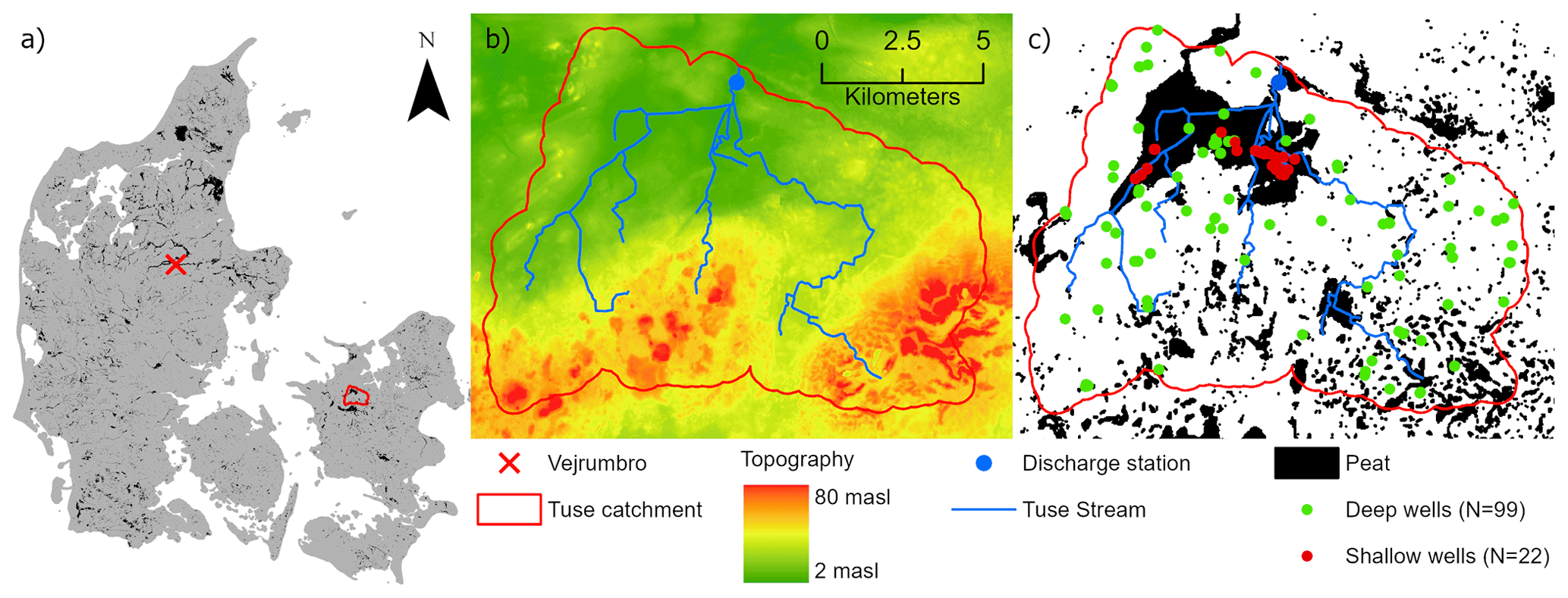
Figure 1 (a) Location of Tuse Stream catchment and the Vejrumbro site, (b) topography and stream network of Tuse Stream catchment, m a.s.l.: meter above sea level, (c) location of organic soil and observation wells in the Tuse Stream catchment.

Shallow WTD in the drained organic soils is monitored in 22 groundwater wells (2–3.5 m deep) (Fig. 1c). The wells are fully screened and WTD is automatically logged with pressure transducers at an hourly basis (aggregated to daily values) and verified with manual measurements. All WTD data are available in the Danish National Well Database (Jupiter, 2025). In this study, we define the water table depth (WTD) as positive when located below the surface and negative when above the surface. Monitoring data includes additional point measurements and timeseries of groundwater head from 99 deep wells installed in mineral soils throughout the catchment (Fig. 1c). In the model setup, water extraction in 40 abstraction wells is included based on data from the Danish National Well Database in May 2020 (Henriksen et al., 2020) and implemented as yearly mean abstraction evenly distributed on the daily model timesteps. Daily discharge is monitored at the catchment outlet at Tuse Stream (Fig. 1b).

2.2 Hydrological modelling

The focus of the hydrological modelling in this study is to adequately simulate shallow groundwater levels and their dynamics for the peatland area in the Tuse Stream catchment. The fen peatland in Tuse Stream catchment is largely fed by groundwater discharge from the upstream catchment, emphasizing the need to develop a coupled groundwater-surface water model at catchment scale. In addition, the objective of utilizing the model for climate change impact assessments requires a catchment scale approach with a deep groundwater component to represent changes in groundwater and surface water discharge to the peatland as well as changes in the boundary conditions. The catchment scale approach also facilitates the combined calibration and evaluation of the total water balance and peatland WTD by constraining the model with observed streamflow at the outlet as well as peatland groundwater level dynamics.

The model is set up as a transient, distributed, coupled surface-groundwater model and executed within the hydrological modeling framework MIKE SHE (DHI, 2022; Graham and Butts, 2005). MIKE SHE combines full 3D groundwater flow coupled with a gravity flow module in the unsaturated zone, 2D overland flow and 1D river flow routing in streams (DHI, 2019) (Fig. S1). The simplified gravity flow module for unsaturated flow assumes a uniform vertical gradient and ignores capillary forces but provides a suitable solution for the time varying recharge to the groundwater table based on precipitation and evapotranspiration (DHI, 2022).

The model is a modified sub-model of the National Hydrological Model of Denmark (DK-model), developed at the Geological Survey of Denmark and Greenland (GEUS) (Henriksen et al., 2020; Stisen et al., 2019). The geological model is interpreted in a horizontal 100 m grid. The numerical model is calibrated in the same 100 m resolution, with the saturated zone consisting of 11 computational layers of varying thickness. The top model layer has a uniform thickness of 2 m, which is also applied to the peat layer areas. The bottom level of the groundwater model is defined by the prequaternary chalk that underlies the Island of Zealand, which in the Tuse Stream catchment is located in a depth of approximately 150–250 m below surface.

The time-varying constant head boundary conditions at the sub-model boundary are defined from the operational National Hydrological Model setup (Henriksen et al., 2020). The observed forcing data of precipitation, temperature and reference evapotranspiration are provided by the Danish Meteorological Institute (DMI) as gridded daily data in 10 km resolution for precipitation and 20 km resolution for evapotranspiration and temperature (Scharling, 1999a, b; Stisen et al., 2011). The model employs a maximum timestep of one day, at which the meteorological variables are fed into the model. The model was provided with a hotstart file from an initial model run.

Spatial and temporal distributions of root depth and leaf area index (LAI) are based on classes (Fig. S2 and Table S1) where the peat, forest, agricultural and open nature land use classes have yearly cycles of LAI and root depth (Fig. S3). Likewise, soil type is spatially distributed (Fig. S2) and based on the three classes peat, sand and clay (Table S2). In the vertical direction, the soil columns in the unsaturated zone module are divided into 40 cells from top to bottom; 30 × 0.1, 5 × 1 and 5 × 5 m. Technically, the unsaturated zone is parameterized to 33 m depth, but during simulation limited to the top of the simulated groundwater table. We implemented uniform vertical water retention characteristics of peat, while clay and sand water retention characteristics were defined separately for the depths 0–30 cm (horizon A), 30–70 cm (horizon B) and > 70 cm (horizon C). Soil parameterization is freely adapted from Børgesen et al. (2009) and detailed in Table S3.

MIKE SHE allows incorporation of drainage systems, representing both artificial and natural drains. The drainage system bypasses the slow water movement in aquifers by providing a short-cut from e.g. the agricultural field to the nearest stream. The amount of water routed by drains from the saturated zone to local surface water bodies is calculated using a linear reservoir model, where the difference between groundwater head and drain level is multiplied by a drain time constant (dt). The drain level is defined by a drain depth (dd) set relative to surface level. Hence, drainage in any given model cell only occurs if the simulated groundwater level exceeds the drainage level (DHI, 2022). The drain time constant and drainage depth in each model grid cell are distributed across the model domain according to the five land use classes (Fig. S2 and Table S1).

The model parameter sensitivity analysis and subsequent calibration prioritized parameters affecting the shallow WTD in the peat soil and the overall water balance in the catchment. A list of model parameters can be seen in Table S3. Parameter values not included in the calibration process are obtained from the National Hydrological Model parametrization.

2.3 Calibration method

We used the Pareto Archived Dynamically Dimensioned Search (PADDS) algorithm (Asadzadeh and Tolson, 2013) available within the optimization toolkit Ostrich (Matott, 2019). PADDS is a multi-objective optimizer and obtains the pareto front across multiple objective function groups, enabling post-weighting of individual objective functions. Throughout the calibration routine, Ostrich minimized the weighted sum of squared error (WSSE) of each of the objective function groups. The PADDS algorithm was run with the user settings of maximum 1000 iterations. The period 2010–2013 was used as a calibration spin-up period and the model performance was evaluated for the 2014–2023 calibration period.

Calibration was performed against three objective function groups as defined in Table 1. The KGE_{WTD_modified} objective group is used to optimize the model performance with respect to the WTD in peatlands. KGE is the Kling-Gupta Efficiency (Gupta et al., 2009) and consists of three terms: the Pearson correlation coefficient r, a term representing the measure of variability α and a bias term β (Table 1). In KGE, β is a unitless measure of the bias specified as the ratio between the sum of simulated and observed values. As we use KGE to optimize the WTD (and not hydraulic head), the operational sign can be both negative (water table above surface/inundation) and positive (water table below surface), violating the idea of optimizing β as the ratio of sums of values with possibly alternating operational signs. Therefore, we are using KGE_{WTD_modified} where β is replaced by the mean error (ME) (Table 1). This modification requires that the order of magnitude of the ME_WTD is comparable to the errors on the other terms in KGE. In our case this is ensured by the fact that the mean observed WTD values range between approximately 0.3–0.6 m, resulting in ME_WTD values typically below 0.5 m. Alternatively, the ME_WTD term could be scaled within the KGE_{WTD_modified} equation.

The calibration using the KGE_{WTD_modified} as objective function group aims at achieving the best overall agreement between simulated and observed WTD. However, during first calibration experiments, we found that this objective function group primarily focuses on the temporal dynamics of WTD. To improve the representation of the spatial variability of the mean WTD, the correlation coefficient (r_spatial) was included as an additional objective function group (Table 1).

KGE_qME_headME_amp is an objective function group that combines three performance criteria: the Kling-Gupta Efficiency performance criterion for discharge (KGE_q), the mean error of hydraulic head in deeper aquifers (ME_head) and the mean error of annual amplitude of hydraulic head in the deeper aquifers (ME_amp). For a detailed description of the implementation of ME_amp as objective function see (Henriksen et al., 2020). This objective function group was included to optimize the overall water balance and streamflow dynamics expressed through the discharge at the catchment outlet (KGE_q), to match the general water level in the deeper aquifers across the catchment (ME_head), and to match the natural seasonal variations in hydraulic head (ME_amp). As the metrics of KGE_q, ME_head and ME_amp are combined into one objective function group, we need to weigh the observations, to ensure that KGE_q, ME_head and ME_amp affect the objective group of KGE_qME_headME_amp approximately equally. This was done based on WSSE from a model run with initial parameter values.

Table 1 Objective functions metrics. KGE stands for Kling-Gupta Efficiency.

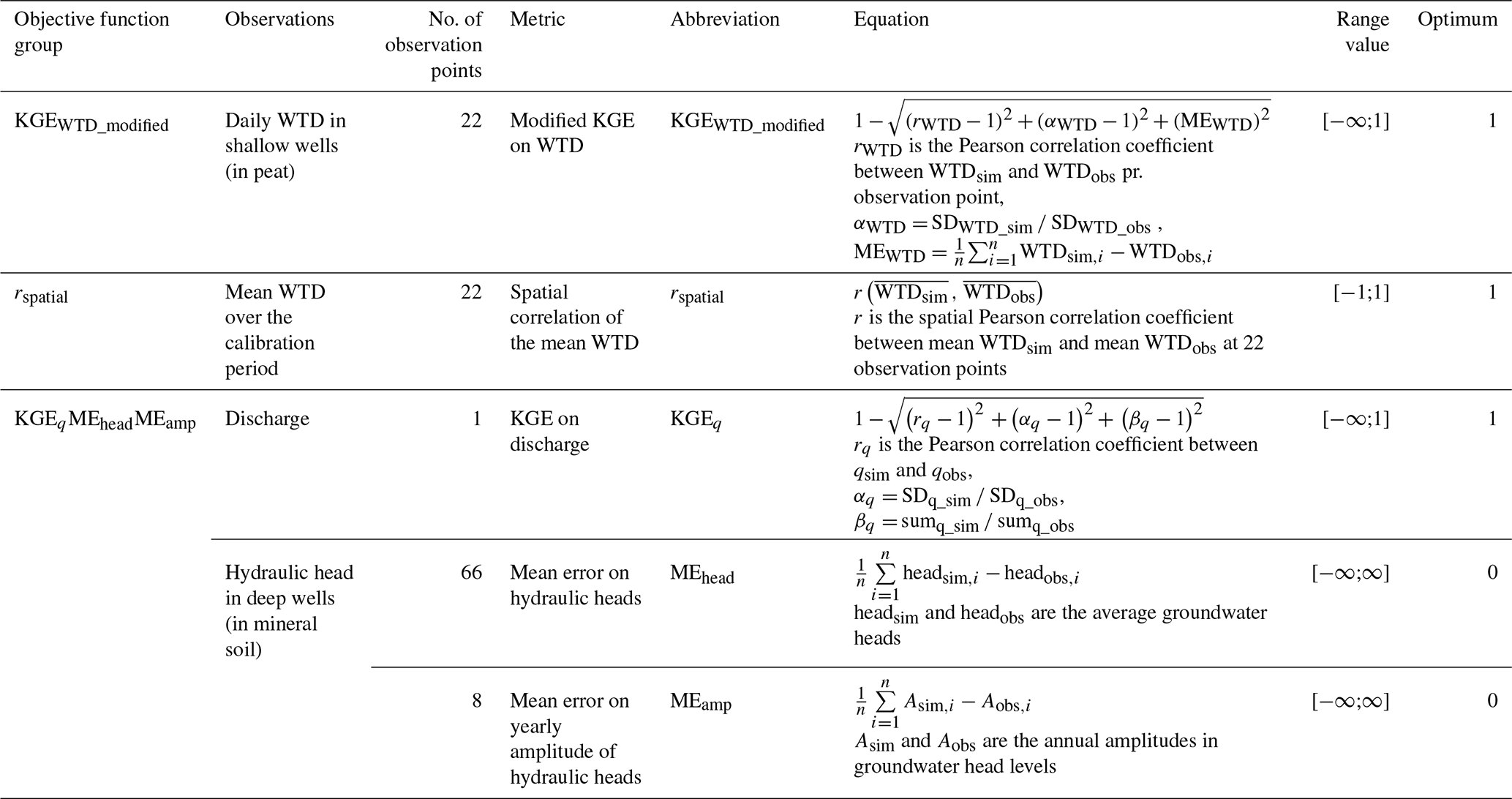
WTD: water table depth (m), q: discharge [m s⁻¹], head: hydraulic head (m), A: amplitude (m).

A local sensitivity analysis based on initial parameter values from Table S4 was performed and values of composite scaled sensitivity (CSS) were obtained. Selection of free calibration parameters were based on the criterion that parameters were included if their CSS was larger than 0.05 × CSS of the parameter with the highest CSS. The resulting 11 free parameters are indicated with grey in Table S4. Other parameters were kept at the values listed in Table S4 or tied to the calibration parameters.

2.4 Hydrological simulations of historical and future climate

The calibrated hydrological model was run for the historical simulation period of 1990–2023 using observed climate forcing data (Scharling, 1999a, b; Stisen et al., 2011). Future hydrological projections are derived from simulations using the hydrological model forced by climate model projections, including precipitation, air temperature (T_air), and potential evapotranspiration. The resulting impacts on groundwater levels, as simulated by the hydrological model, are evaluated. We used 17 climate models (Table S5) with the Representative Concentration Pathway 8.5 (RCP8.5), which represents the RCP scenario (2.6–8.5) leading to the highest emissions and strongest impact of climate change. The climate model outputs are generated and bias corrected by Pasten-Zapata et al. (2019), and the Global and Regional Circulation (GCM, RCM) models originate from the Euro-CORDEX project (Jacob et al., 2014).

The climate simulations cover three 30-year periods: the reference period (1991–2020), the mid-century (2041–2070) and the end-century (2071–2100). All 51 climate simulations (17 climate models × 3 periods) were first run using the initial potential head from the national model climate simulations (Henriksen et al., 2020). Subsequently, they were rerun using the mean potential head for the respective 30-year period as the initial potential head.

2.5 Empirical CO₂ emission models

2.5.1 Implementation of annual CO₂ emission model

Recent studies established a functional relationship between the annual NECB for CO₂ and the mean annual WTD (Koch et al., 2023; Tiemeyer et al., 2020) by fitting a nonlinear Gompertz function. Like in Koch et al. (2023) and Tiemeyer et al. (2020), this study considers NECB as only CO₂ fluxes, excluding methane (CH₄) and other carbon exports such as dissolved or particulate organic carbon. We apply the WTD functional relationship for CO₂ from Koch et al. (2023), which is fitted to Danish flux data, and refer to it as the Annual WTD model. The Annual WTD model demonstrates a systematic relationship in which CO₂ flux from NECB increases with annual WTD in the interval between 7 and 50 cm, above which an asymptotic level of 10 Mg CO₂-C ha⁻¹ yr⁻¹ is reached (Koch et al., 2023). The Annual WTD model is therefore not sensitive to changes in WTD deeper than approximately 50 cm. At WTD levels less than 7 cm, the Annual WTD model suggests CO₂ uptake; however, this element is not included in our analysis which only models CO₂ emission.

2.5.2 Derivation and implementation of daily CO₂ emission model

For our empirical model to predict daily soil CO₂ fluxes (fCO₂) we assume that the WTD dependent NECB (Tiemeyer et al., 2020; Koch et al., 2023) is driven mainly by the response of soil respiration to WTD and T_air, as gross primary photosynthesis (GPP) and aboveground autotrophic respiration is mostly dependent on light availability and plant phenology (Rodriguez et al., 2024). This allows scaling to match the NECB magnitude but maintains integrity in the regulation of WTD on soil CO₂ fluxes.

Using a unique and comprehensive coupled dataset (Nielsen et al., 2026) of daily mean net soil CO₂ fluxes, T_air and WTD for six spatial replicate measurement points, we develop a coupled temperature and WTD dependent empirical soil CO₂ flux model, hereafter referred to as the Daily WTD-T_air model. The model essentially scales the WTD-fCO₂ relation to T_air. The dataset Nielsen et al. (2026) is from a drained fen, called Vejrumbro (Fig. 1), with similar characteristics (soil type, climate, land use history) as the peat area in the Tuse Stream catchment (see methodological details in Nielsen et al., 2026). The soil net CO₂ fluxes, WTD and T_air were measured automatically for one year (2022–2023) (Nielsen et al., 2026) and we used a subset of fluxes measured for six spatial replicates 5–6 times per day, resulting in a dataset of 10 950–13 140 individual fluxes covering 365 d (Nielsen et al., 2026).

2.5.3 Implementation of CO₂ flux models

Spatially distributed net soil CO₂ fluxes are calculated at a 100 m scale across the 13 km² contiguous peatland area (Fig. 1) with the Annual WTD model and the Daily WTD-T_air model, respectively, using WTD at a 100 m scale (hectare scale) and a uniform T_air. Afterwards the spatially distributed soil CO₂ fluxes are aggregated to represent the spatial mean of the 13 km² peatland area.

First, we applied the Annual WTD model and the Daily WTD-T_air model for the historical simulation period of 1990–2023, using spatiotemporal distributed WTD from the calibrated hydrological model. Afterwards, the empirical CO₂ models are utilized on each of the 17 climate projections for T_air and WTD. Daily T_air for the Tuse Stream catchment peatland area is taken directly from the 17 bias corrected climate projections, while daily spatial WTD is a model output from the 17 hydrological simulations, when running the hydrological model with the forcing data (precipitation, temperature and evapotranspiration) from the 17 climate projections. Thereby, we are able to quantify the variability in soil CO₂ flux among the 17 climate projections for each of the simulation periods and among the 30 years within each of the simulation periods.

2.6 Design and application of rewetting scenarios

For impact evaluations of peatland management scenarios on the annual CO₂ emissions, we define three rewetting scenarios: A, B and C. These scenarios are implemented through controlled modifications of the simulated WTD in peatland grid cells. This method of representing rewetting scenarios does not involve structural modifications to the hydrological model and assumes changes in WTD without accounting for process-based feedback mechanisms within the coupled surface–subsurface hydrological system. Therefore, the rewetting scenarios cannot be interpreted as real-life management practices. All rewetting scenarios were applied for 1990 to 2023, representing the climatology for this period and generating 34-year time series of rewetted WTD.

The scenarios are meant to illustrate different rewetting impacts on WTD, representing wetter winters (A), uniform shift in WTD (B) and wetter summers (C), but all with the same long-term mean WTD. In Scenario A, the daily groundwater table is elevated when it is above the long-term (34-year) mean water table resulting in unchanged water table levels during summer but an increase in winter. Scenario B uniformly raises the water table by a constant scalar, while Scenario C applies the same scalar increase to water table while simultaneously reducing the annual amplitude by half. The modifications of the simulated WTD are implemented using the following equations:

$$\begin{array}{}\text{(1)}& {\displaystyle }{\mathrm{WTD}}_{i,\mathrm{rewet}\mathrm{A}}=\left\{\begin{array}{ll}{\mathrm{WTD}}_i,& \text{if}{\mathrm{WTD}}_i\ge \stackrel{\mathrm{‾}}{\mathrm{WTD}}\\ {\mathrm{WTD}}_i+\mathrm{2.5}\cdot (\stackrel{\mathrm{‾}}{\mathrm{WTD}}-{\mathrm{WTD}}_i),& \text{if}{\mathrm{WTD}}_i<\stackrel{\mathrm{‾}}{\mathrm{WTD}}\end{array}\right.\text{(2)}& {\displaystyle }{\mathrm{WTD}}_{i,\mathrm{rewet}\mathrm{B}}={\mathrm{WTD}}_i-\left(\stackrel{\mathrm{‾}}{\mathrm{WTD}}-\stackrel{\mathrm{‾}}{{\mathrm{WTD}}_{\mathrm{rewet}\mathrm{A}}}\right)\text{(3)}& {\displaystyle }{\mathrm{WTD}}_{i,\mathrm{rewet}\mathrm{C}}=\stackrel{\mathrm{‾}}{{\mathrm{WTD}}_{\mathrm{rewet}\mathrm{B}}}+\mathrm{0.5}\cdot \left({\mathrm{WTD}}_{i,\mathrm{rewet}\mathrm{B}}-\stackrel{\mathrm{‾}}{{\mathrm{WTD}}_{\mathrm{rewet}\mathrm{B}}}\right)\end{array}$$

where WTD_i,rewet A, WTD_i,rewet B and WTD_i,rewet C is the daily WTD in a grid cell for rewetting scenario A, B and C, respectively. WTD_i is the daily WTD in a grid cell from the calibrated hydrological model. $\stackrel{\mathrm{‾}}{\mathrm{WTD}}$ is the long-term (34-year) mean WTD in a grid cell from the historical period of the calibrated hydrological model. $\stackrel{\mathrm{‾}}{{\mathrm{WTD}}_{\mathrm{rewet}\mathrm{A}}}$ and $\stackrel{\mathrm{‾}}{{\mathrm{WTD}}_{\mathrm{rewet}\mathrm{B}}}$ are long-term (34-year) mean WTD in a grid cell from the rewetting scenario A and B, respectively.

2.7 Uncertainty of future CO₂ emission estimates

We applied a bootstrap resampling approach to estimate the uncertainty in the mean values of soil CO₂ flux. Specifically, we resampled the means over the 17 climate models, each containing 30 annual values, with replacement. This process was repeated 10 000 times to construct bias-corrected and percentile-based 95 % confidence intervals around the bootstrapped means.

3 Results

3.1 Hydrological model

3.1.1 Calibration of the hydrological model

The model calibration, running 1000 model evaluations based on three objective function groups, using Ostrich ParaPADDS optimizer with 40 parallel model executions, took ∼ 24 h on a Xeon Et-4850 @2,20 GHz Server. The calibration resulted in 203 non-dominated solutions forming a three-dimensional pareto front. Figure 2 presents scatterplots of the three objective functions, illustrating the trade-offs between them. Especially, there is a clear trade-off between the two objective functions addressing temporal dynamics (KGE_{WTD_modified}) and spatial dynamics (r_spatial), as illustrated in Fig. 2a.

The number of non-dominated solutions and the trade-offs illustrate that several parameter sets can be considered and that an ensemble of parameter sets could be selected. For the purpose of further analysis and climate change impact assessments, however, we select one balanced solution from the non-dominated solutions, through a stepwise procedure. First, a pre-screening was performed with performance criteria for WTD of KGE_{WTD_modified} larger than 0.6, for discharge of KGE_q larger than 0.6 and for hydraulic head in deeper wells of ± 1 m, for ME_head and ME_amp, respectively. Afterwards, the balanced parameter set was selected as the solution with the highest spatial correlation (r_spatial).

The selection procedure was designed to prioritize accurate simulation of the temporal dynamics of peatland WTD, while maintaining strong performance across additional objective functions and maximizing spatial correlation accuracy. Initial calibration efforts indicated that achieving a KGE_{WTD_modified} value greater than 0.6 was necessary to ensure an adequate alignment between the simulated and observed WTD time series.

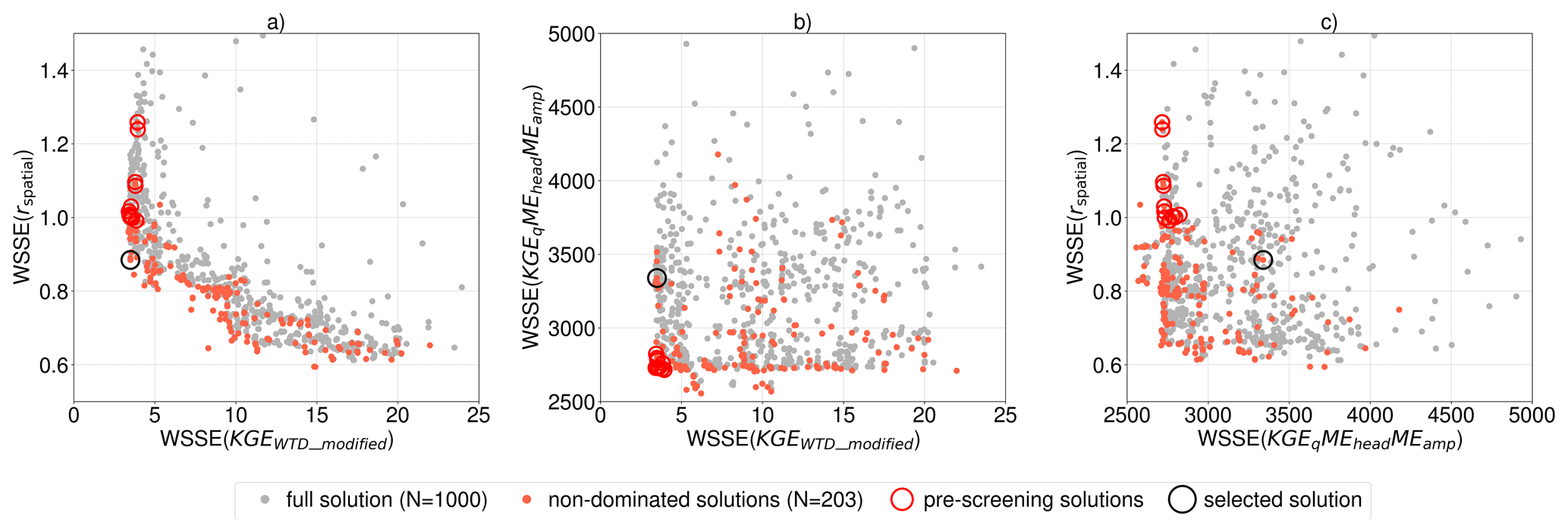
Figure 2 Scatterplots of WSSE (weighted sum of squared errors) for the three objective function groups in the calibration. Pareto front for 1000 model evaluations.

3.1.2 Hydrological model performance

Model performance metrics for the selected solution are summarized in Table 2. The KGE_qME_headME_amp objective function is separated into individual contributions from the metrics KGE_q, ME_head and ME_amp. Additionally, Table 2 shows the three metrics which make up the KGE_{WTD_modified}: r_WTD, α_WTD and ME_WTD. In general, the model performs well with a KGE_{WTD_modified} in peat of 0.64, a KGE_q of 0.63, a ME_head for the deep wells of 0.75 m and a ME_amp for the deep wells of 0.51 m for the selected solution. However, the correlation coefficient for the spatial variability (r_spatial) is poor with a value of 0.06. The model optimization achieves solid metrics on all the three components of KGE_{WTD_modified}. The mean bias of WTD across all shallow peatland observation wells (ME_WTD) is only 8 cm (Table 2).

Table 2 Hydrological model performance.

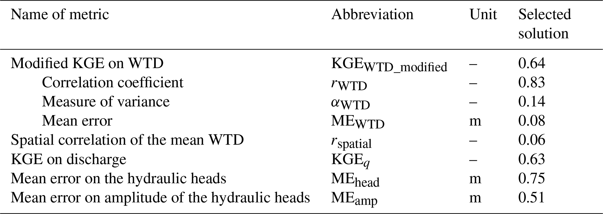
Though the model obtains a relatively small mean error, it largely underestimates the spatial variability in WTD. The observed mean WTD variability across the 22 monitoring wells (SD = 16.5 cm) is considerably higher than that observed in the simulations (SD = 6.8 cm). Even though the model performance on KGE_{WTD_modified} was generally good, it proved difficult to reproduce the spatial variation in mean WTD.

To investigate the underestimation of spatial variability in WTD, we analyzed several spatial variables considered relevant for explaining the observed variability in WTD: peat thickness, topography and proximity to water bodies. However, no clear correlation was found between these spatial variables and the mean observed WTD or model bias, as all had a correlation coefficient smaller than 0.34. See Table S6.

3.1.3 Historical simulations of water table depth

The simulated WTD, generated by the calibrated hydrological model driven by historical climate for the period 1990–2023, adequately represent both the observed seasonal patterns of WTD and their short-term responses to precipitation events. Figure 3 shows the time series of WTD from two individual monitoring wells as a typical example of the temporal match between observed and simulated WTD.

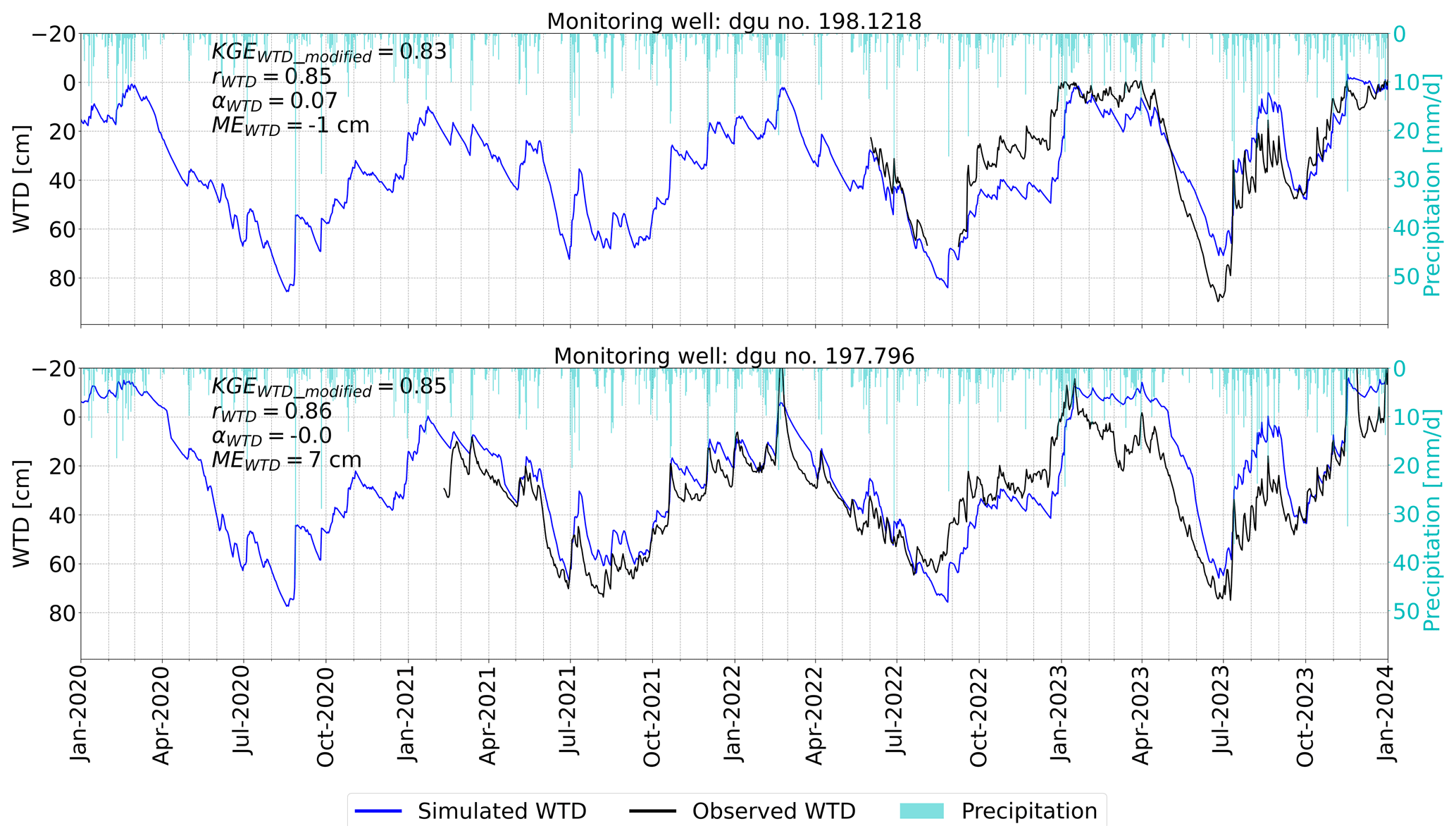
Figure 3 Example of observed and simulated timeseries for water table depth (WTD) for monitoring wells dgu no. 198.1218 and dgu no. 197.796. Including metrics for these wells.

3.1.4 Meteorological climate predictions

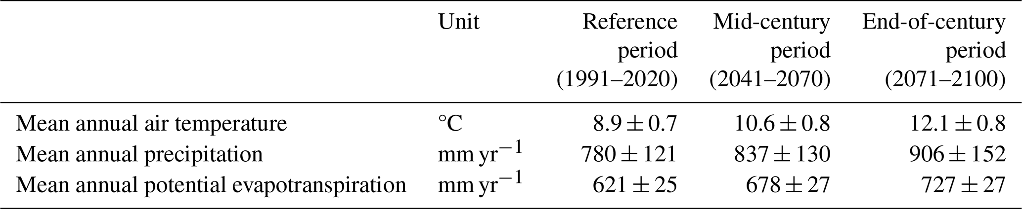
Changes in precipitation, temperature and evapotranspiration patterns in future climate projections for Denmark generally indicate an increase in both temperature and annual precipitation. Table 3 presents the mean air temperature, mean annual precipitation and mean potential evapotranspiration derived from the 17 climate projections across the three simulation periods.

Table 3 Mean ± SD (n=17) of annual air temperature, precipitation and potential evapotranspiration from the 17 climate models during the three simulation periods.

3.1.5 Hydrological climate predictions

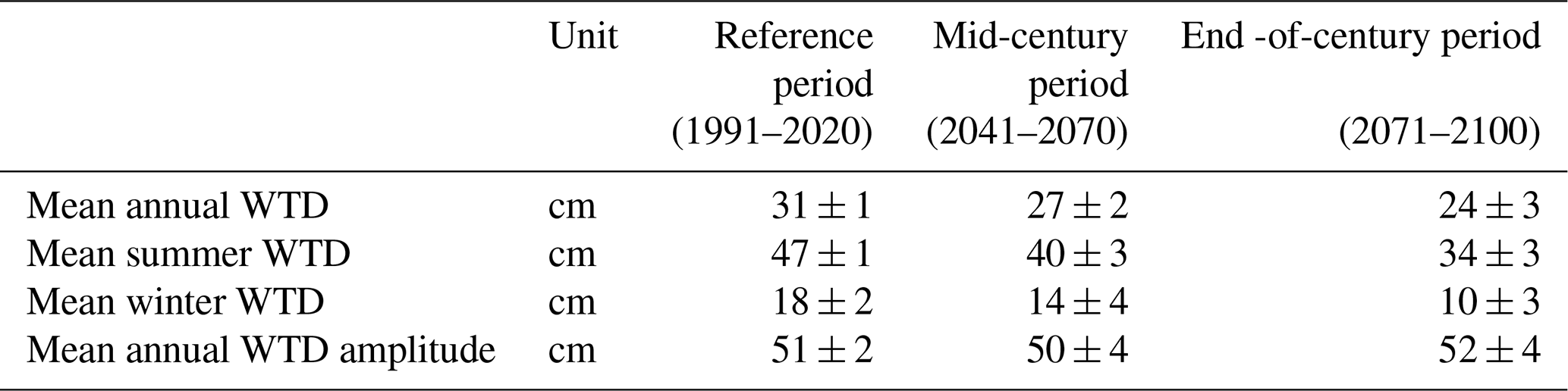
Climate simulations using the hydrological model indicate a decreasing trend in mean annual WTDs (Table 4), resulting in a shallower annual mean groundwater table in future climate conditions. Both summer and winter mean WTDs are projected to be closer to the surface, suggesting generally wetter conditions. The mean annual amplitude of WTD remains unchanged under future climate scenarios (Table 4), indicating that there is no greater seasonal drawdown of the water table during summer, although the duration of the drawdown period may be extended.

Table 4 Statistics of WTD when using the hydrological model for climate simulations. Mean ± SD (n=17) over the 17 climate models during the three simulation periods. Summer is June, July and August, Winter is December, January and February. The amplitude is based on the monthly means of WTD to avoid outliers.

3.2 Derivation of empirical daily soil CO₂ flux model

An analysis of the Vejrumbro dataset indicated a clear temperature dependency on the relation between soil CO₂ flux (fCO₂) and WTD. The Vejrumbro dataset was resampled to daily means of WTD, T_air and soil CO₂ flux across the six spatial replicate measurement points omitting data from days with less than 24 flux measurements. This resulted in a dataset with 231 daily observations for each of fCO₂, WTD and T_air distributed evenly over a year. Traditionally, empirical emission models for ecosystem respiration (R_eco) are fitted to soil temperature. However, due to the strong linear relationship between daily soil temperature and daily air temperature at the Vejrumbro site (r = 0.96, p-value < 0.001) (Fig. S4), T_air was used as a proxy for soil temperature when fitting the Daily WTD-T_air model. This use of air temperature also facilitates upscaling and omits the need for projecting soil temperatures under climate change scenarios.

To investigate how the WTD-fCO₂ relation scales with temperature, we binned daily soil CO₂ flux into five temperature intervals: < 4 °C (n=39), 4–8 °C (n=32), 8–12 °C (n=52), 12–16 °C (n=70) and > 16 °C (n=38) and applied a linear regression model (y=ax) with the intercept constrained at zero within each temperature bin. The regressions were constrained to pass through the origin, reflecting the assumption that soil CO₂ flux is zero when the WTD is zero. Thereby, the relationship between fCO₂ and WTD within each temperature bin was modeled using a linear regression of the form:

$$\begin{array}{}\text{(4)}& f{\mathrm{CO}}_{\mathrm{2}}=a\cdot \mathrm{WTD}\end{array}$$

where fCO₂ represents soil CO₂ flux [Mg CO₂-C ha⁻¹ d⁻¹], a denotes the fitted slope and WTD is water table depth [cm], with positive values indicating depths below the surface.

This analysis revealed an increasing slope, i.e. sensitivity of soil CO₂ flux to changes in WTD, with rising temperature (Figs. S5 and Fig. 4a), indicating that the WTD-fCO₂ slope (a) can be modelled as a linear function of temperature (T_air) (Fig. 4b):

$$\begin{array}{}\text{(5)}& a=b\cdot T_{\mathrm{air}}+c\end{array}$$

Combining these relationships yields a simple model of the soil CO₂ flux:

$$\begin{array}{}\text{(6)}& f{\mathrm{CO}}_{\mathrm{2}}=b\cdot T_{\mathrm{air}}\cdot \mathrm{WTD}+c\cdot \mathrm{WTD}\end{array}$$

where T_air [°C] is the temperature, b [Mg CO₂-C ha⁻¹ d⁻¹ cm⁻¹ °C⁻¹] and c [Mg CO₂-C ha⁻¹ d⁻¹ cm⁻¹] are empirical constants.

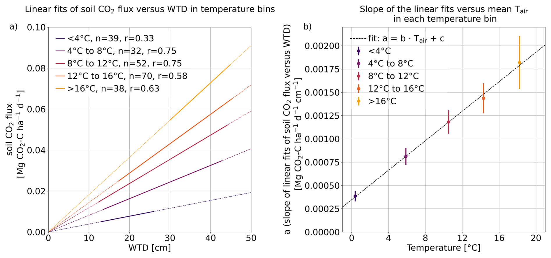
Figure 4 (a) linear models of soil CO₂ flux vs. water table depth (WTD) in air temperature bins. The thicker segment of the line represents the range of data used to derive the fitted model. n is the number of daily observations of soil CO₂ flux in each temperature bin. r is Person correlation coefficient. Raw data behind the linear regressions can be seen at Fig. S5. (b) Slope (incl. uncertainty) (of the linear fit of soil CO₂ flux versus WTD) versus observed mean temperature in each temperature bin.

Having established a suitable form of the empirical soil CO₂ flux equation, we used nonlinear least squares fit to estimate the b and c parameters based on the daily soil CO₂ flux, T_air and WTD (without temperature bins). This method minimizes the residual sum of squares between the observed soil CO₂ flux and the Daily WTD-T_air model. The resulting fitted model demonstrated a significant correlation to the observed data (r = 0.78, p-value < 0.001, RMSE = 0.021 Mg CO₂-C ha⁻¹ d⁻¹) (Fig. S6) with daily soil CO₂ flux increasing in response to rising WTD and T_air (Fig. S7). The fitted empirical constants are as follows: b = 8.32 × 10⁻⁵ Mg CO₂-C ha⁻¹ d⁻¹ cm⁻¹ °C⁻¹, c = 3.33 × 10⁻⁴ Mg CO₂-C ha⁻¹ d⁻¹ cm⁻¹.

The Daily WTD-T_air model predicts the highest soil CO₂ flux under conditions of simultaneously high T_air and WTD, where a high WTD refers to a water table located furthest below the surface (dry conditions). The multiplicative Daily WTD-T_air model demonstrated a moderate fit to the soil CO₂ flux data, with a R² of 0.61. To assess the individual contributions of the predictor variables, we also computed the R² between CO₂ flux and T_air and WTD separately. This was done using a constructed dataset that included all combinations of WTD and T_air within the model range. This resulted in R² values of 0.34 for T_air and 0.54 for WTD (Table S7). These values reflect the explanatory power of each variable in isolation.

Despite the significant variability in the observed NECB used for the Annual WTD model (Fig. 5) it is considered to represent a robust mean as it is based on multiple sites and years for Danish and German conditions. Compared to the Annual WTD model both the measured soil CO₂ flux (12.9 Mg CO₂-C ha⁻¹ yr⁻¹ (green circle)) and the Daily WTD-T_air simulated soil CO₂ flux (13.6 Mg CO₂-C ha⁻¹ yr⁻¹ (not shown)) at Vejrumbro are above the corresponding fitted value of NECB (8.7 Mg CO₂-C ha⁻¹ yr⁻¹ (orange circle)) based on an annual WTD of 29 cm, but still within the range of observed NEBCs used for fitting the Annual WTD model (Fig. 5). This may be explained by the methodology of flux measurements at Vejrumbro that did not consider GPP (CO₂ uptake) and therefore are expected to result in higher net CO₂ fluxes. In order to align the Daily WTD-T_air model to the level of the Annual WTD model where GPP is included, a scaling factor based on the above differences (f_scaling=0.64) was applied to Eq. (6) to account for lack of GPP in the soil CO₂ fluxes used for empirical model development. Applying this scaling factor, we seek to avoid the risk of overestimating emissions when applying the Daily WTD-T_air model at other locations.

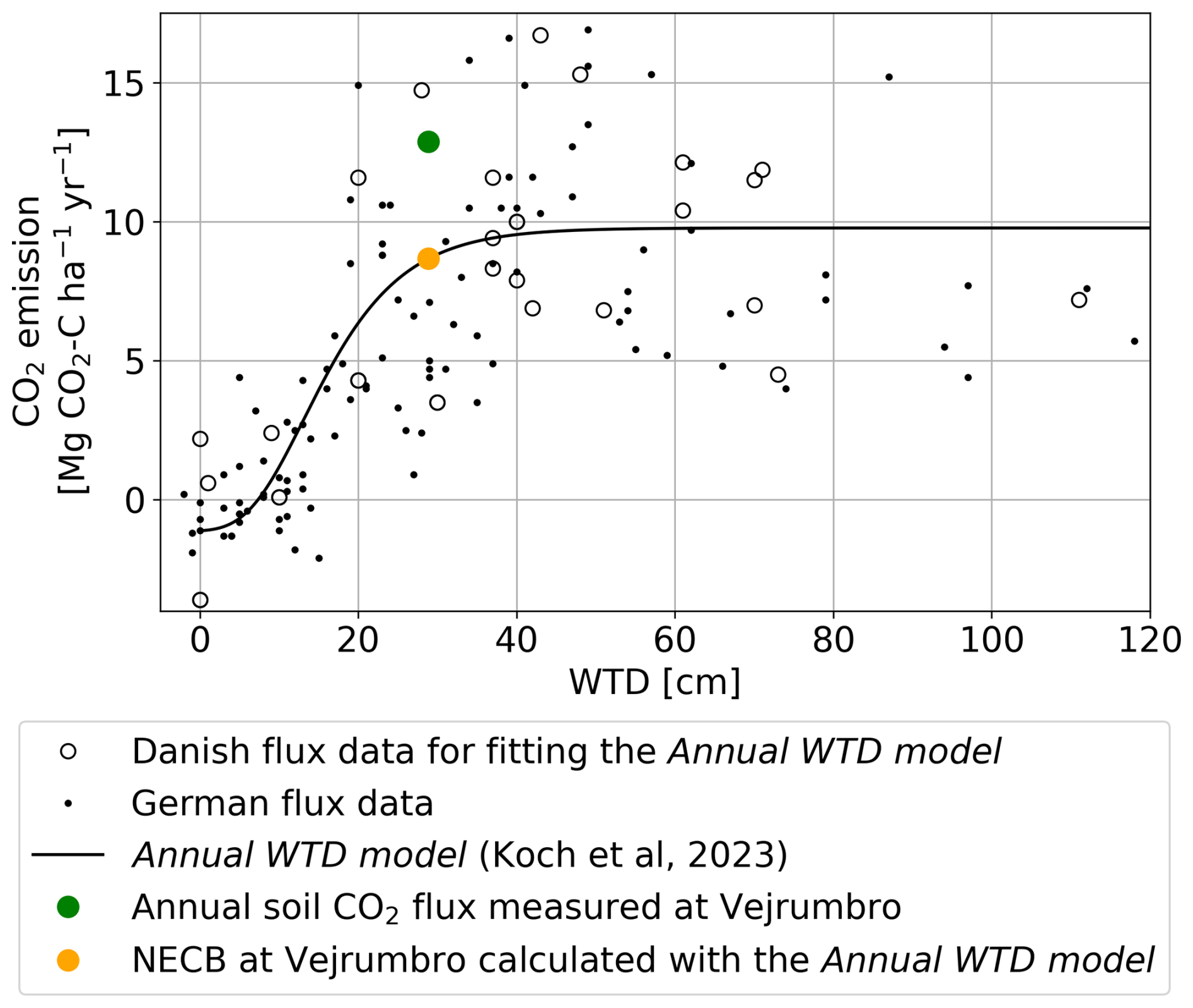
Figure 5 The Annual WTD model together with the Danish flux data of annual NECB and WTD data underlaying the model (Koch et al., 2023). German flux data are included for comparison (Tiemeyer et al., 2020). Colored circles are measured and calculated soil CO₂ flux and NECB for the Vejrumbro dataset, so the colored circles represent the year 2022–2023.

The Vejrumbro dataset used for fitting the Daily WTD-T_air model was limited to a maximum WTD of 47 cm and maximum T_air of 21 °C (Fig. S7). Outside this range, the predictions of the Daily WTD-T_air model exhibits increased uncertainty. At the same time, it is generally understood that the upper portion of the peat layer drives the net CO₂ emissions observed at the surface. Therefore, the extrapolation of WTD in the Daily WTD-T_air model must be constrained. The Daily WTD-T_air model should be sensitive within a WTD range comparable to the expected daily variation in the Annual WTD model, which also reaches an fCO₂ asymptotic at deeper water tables. In the Annual WTD model, the Annual NECB reaches 90 % of its maximum asymptotic level at a mean annual WTD of 30 cm (Fig. 5). The mean annual WTD results from intra-annual (within year) WTD variation described by the annual amplitude. The mean annual amplitude (based on monthly means) is 65 cm, across the 22 observed WTD time series in the Tuse Stream catchment used for calibrating the hydrological model. We assume that a mean annual WTD of 30 cm originates from an annual WTD variation with a similar amplitude. Therefore, we assume that the WTD range of the Daily WTD-T_air model is 30 + $\mathrm{65}/\mathrm{2}$ cm = 62.5 cm. For the T_air range, it is assumed that the sensitivity continues until 25 °C, which is a daily average value very rarely occurring, even in future climate projections. Thus, when applying the Daily WTD-T_air model, daily WTD values and T_air values were truncated, setting WTD and T_air to 62.5 cm and 25 °C, respectively, when exceeding those thresholds.

In both the Daily WTD-T_air model and the Annual WTD model, CO₂ fluxes are constrained so that the model does not simulate negative fluxes or carbon uptake (Gyldenkærne et al., 2025).

3.3 CO₂ emissions from peatlands

3.3.1 CO₂ emissions throughout the historical simulation period

The long-term mean of the emission factor for the Tuse Stream catchment peat area is 8.0 ± 0.8 Mg CO₂-C ha⁻¹ yr⁻¹ (mean ± SD, n=34) when using the Annual WTD model and 8.8 ± 1.6 Mg CO₂-C ha⁻¹ yr⁻¹ (mean ± SD, n=34) when using the Daily WTD-T_air model (Table 5).

Table 5 Long-term mean water table depth (WTD), long-term mean annual WTD amplitude (based on monthly means of WTD to avoid outliers) and long-term soil CO₂ flux, throughout the historical period and the three modified 34-year WTD time series of rewetting scenarios. Mean ± SD is based on the 34 years of the historical period (1990–2023).

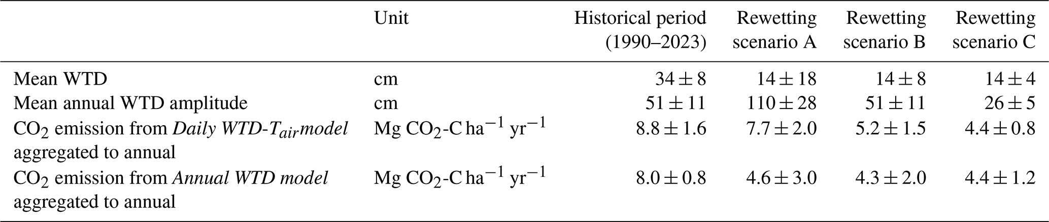
Figure 6 shows T_air, as wells as the spatial mean of WTD and CO₂ emissions across the peatland, as simulated by the Daily WTD-T_air model and the Annual WTD model during the historical period. The CO₂ emissions calculated with the Daily WTD-T_air model (red line in Fig. 6c, d) depend on both the observed daily temperature variability (orange line in Fig. 6a) and simulated intra-annual (seasonal) WTD variability (blue line in Fig. 6b), while the CO₂ emission calculated with the Annual WTD model (black points in Fig. 6d) only depends on the inter-annual (annual means) WTD (blue points in Fig. 6b) and not the temperature.

Inter-annual (between years) variation in CO₂ emission is substantially larger when using the Daily WTD-T_air model (SD = 1.6 Mg C-CO₂ ha⁻¹ yr⁻¹) compared to the Annual WTD model (SD = 0.8 Mg C-CO₂ ha⁻¹ yr⁻¹) (Fig. 6d), as the former captures extreme events, such as periods of high temperature or deep groundwater tables, as well as compound events involving the simultaneous occurrence of both. In contrast, the Annual WTD model is insensitive to temperature and the intra-annual (within year) timing of deep WTD. Moreover, the Annual WTD model imposes an upper limit of 10 Mg CO₂-C ha⁻¹ yr⁻¹ for annual emissions (Koch et al., 2023) (Fig. 5). During the summer of 2018, a compound extreme event occurred, characterized by both high temperatures and deep groundwater table. The annual CO₂ flux for this year shows a 34 % increase when estimated using the Daily WTD-T_air model compared to the Annual WTD model. This discrepancy arises from the Daily WTD-T_air model's ability to account for the prolonged duration of concurrent high temperatures and deep groundwater table conditions throughout the summer (Fig. 6d). Conversely, in 2010, the Daily WTD-T_air model estimates significantly lower annual CO₂ emissions compared to the Annual WTD model (Fig. 6d). This difference is due to the emission model's ability to account for the effects of prolonged periods of low temperatures during the autumn and spring of 2010, leading to a mean annual temperature below the long-term mean, despite summer temperatures being consistent with other years (Fig. 6a). Examples of years with extreme events primarily driven by either WTD or T_air include 1996, which experienced a significant summer decline in groundwater table (Fig. 6b), and 1997, which was characterized by elevated summer temperatures (Fig. 6a). However, neither of these events led to CO₂ emissions as high as those simulated during the compound event of both high temperatures and deep water table in 2018 (Fig. 6).

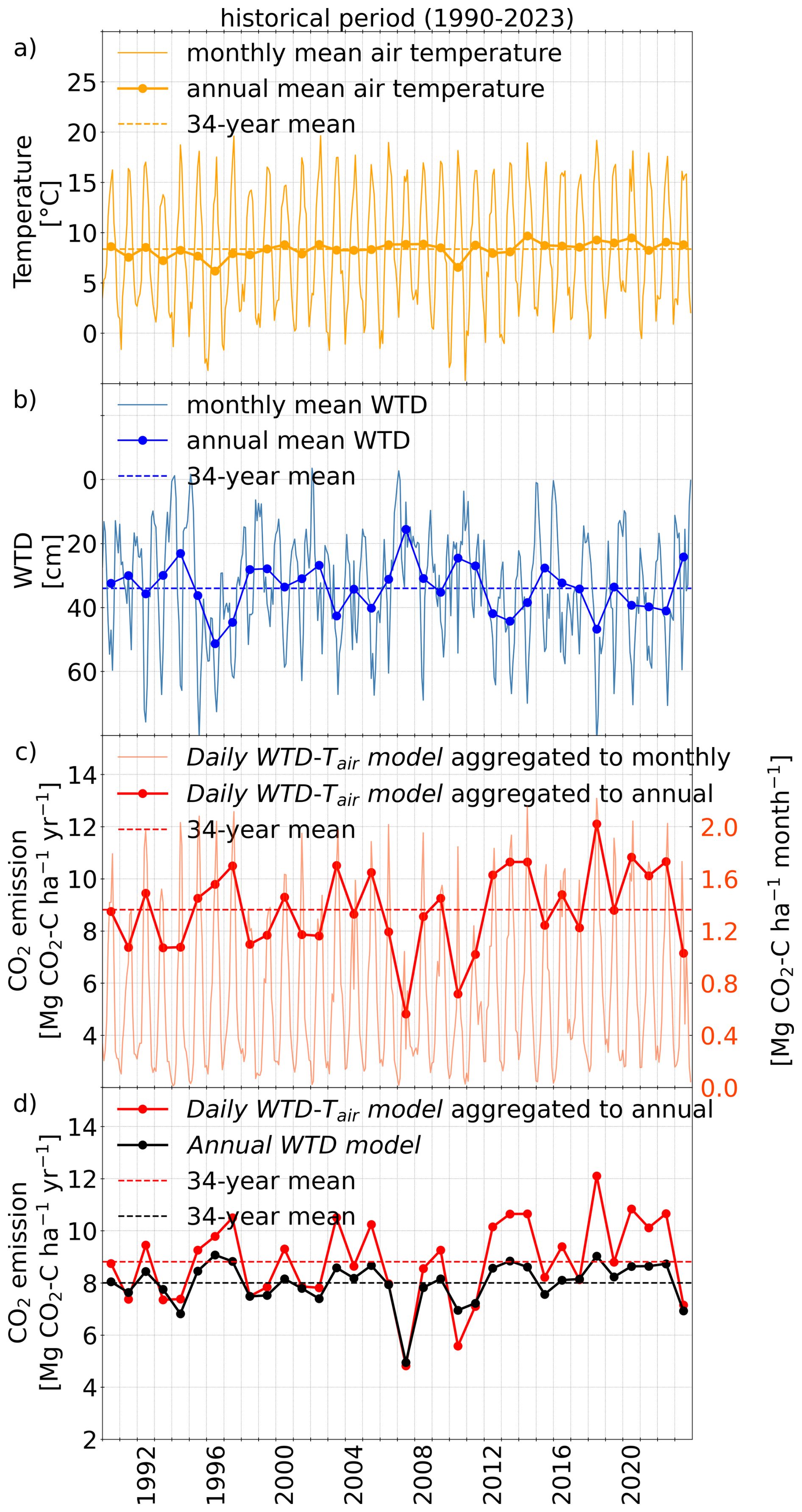
Figure 6 Air temperature (T_air), water table depth (WTD) and soil CO₂ emission for the historical simulation period 1990–2023.

3.3.2 CO₂ emissions under different rewetting scenarios

The rewetting scenarios represent an adjustment to the WTD simulated by the hydrological model over the 34-year historical period, thereby reflecting the climatological conditions prevailing during that time. Across all three rewetting scenarios, the long-term (34-year) mean WTD was raised by 20 cm, from 34 cm to 14 cm below the surface, ensuring a consistent long-term annual mean WTD among the rewetting scenarios (Table 5). Accordingly, the application of the Annual WTD model for estimating CO₂ fluxes result in CO₂ emissions between 4.3 ± 1.2 Mg C-CO₂ ha⁻¹ yr⁻¹ (mean ± SD, n=34) and 4.6 ± 3.0 Mg C-CO₂ ha⁻¹ yr⁻¹ (mean ± SD, n=34) across all rewetting scenarios (Table 5). The mean annual soil CO₂ flux from the three rewetting scenarios, as calculated using the Annual WTD model, are similar but not identical. This is because the Annual WTD model is applied to each of the 34 individual annual mean WTD values rather than to a single long-term mean WTD. The SD of CO₂ emissions calculated using the Annual WTD model in scenario C is markedly lower than in rewetting scenario A and B, reflecting the lower inter-annual (between years) variability in mean annual WTD observed for this scenario (Table 5).

In contrast to the Annual WTD model, the Daily WTD-T_air model captures the simultaneous occurrence of low groundwater table and high T_air during the summer months. Application of this emission model indicates that raising the groundwater table during summer months (rewetting scenario C) yields the greatest reduction potential in soil CO₂ emissions (Table 5), leading to a 50 % decrease in the mean value, from 8.8 ± 1.6 to 4.4 ± 0.8 Mg C-CO₂ ha⁻¹ yr⁻¹ (mean ± SD, n=34) (Table 5). In contrast, management scenarios that primarily target increase in winter water table (rewetting scenario A) exhibit only marginal emission reduction potential (Table 5).

A visual representation of daily soil CO₂ emissions in relation to mean daily temperature during the 34-year historical period under different WTD conditions (Fig. 7) reveals that high summer temperatures are a key driver of CO₂ emissions. WTD observations from the Tuse catchment peatland indicate that, during shorter periods in the warm summer months, the WTD can exceed 80 cm (Fig. 3). These periods with very low summer water table contribute substantially to total CO₂ emissions (Fig. 7).

A rewetting scenario that mainly generates wetter winter conditions (rewetting scenario A) has very limited CO₂ emission reduction. All three scenarios assume that even under rewetting, the peatland WTD will follow a climate driven seasonality and that obtaining zero WTD in summer periods will be difficult by classical nature-based solutions. Rewetting scenario C, which features the greatest increase in summer WTD, achieves the largest reduction in CO₂ emissions (Fig. 7). Permanent wet conditions with WTD at zero would be required to obtain zero CO₂ emission with the developed Daily WTD-T_air model, but under such conditions, methane emissions would also come into play and plant growth would be severely limited.

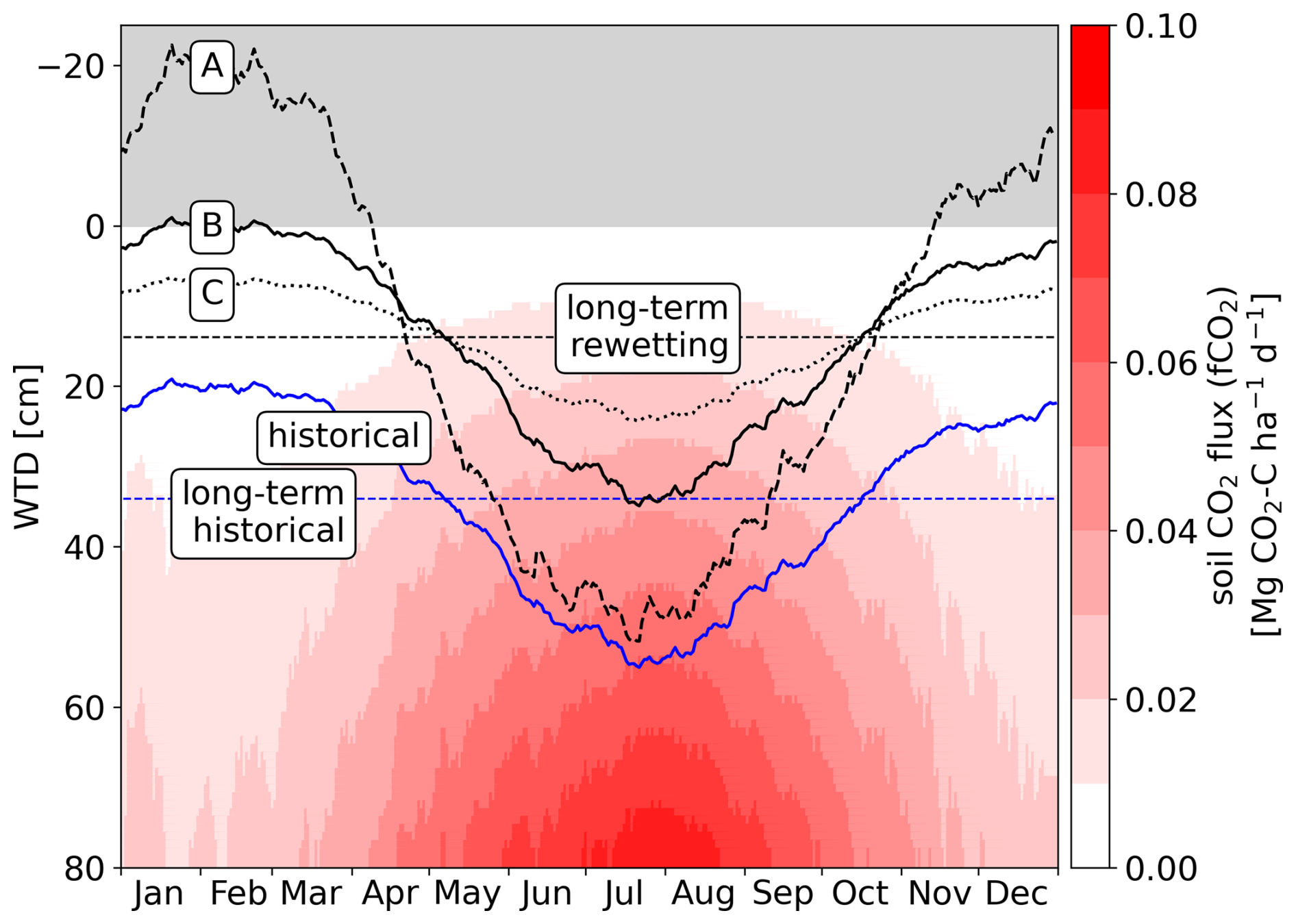
Figure 7 Colormap: Visual representation of the annual distribution of daily surface soil CO₂ flux (fCO₂, CO₂ exchange with atmosphere) under mean daily temperature during the historical period (1990–2023) and for different water table depths (WTD). Curves: solid blue line: simulated daily mean WTD during the historical period and corresponding long-term (34-year) mean WTD, black lines: daily mean WTD for each of the modified 34-year WTD time series of rewetting scenarios (A, B and C) and the corresponding long-term (34-year) mean WTD.

3.3.3 CO₂ emissions across future climate simulation periods

Figure 8 shows the same variables as Fig. 6 but based on a representative climate model simulation instead of the observed climate record, offering a typical example of the development of temperature, WTD and soil CO₂ flux through the reference, mid-century and end-of-century periods based on the RCP8.5 pathway.

The future climate simulations show an increase in both the annual mean temperature and groundwater levels combined with higher maximum summer temperature (Fig. 8a, b, Tables 3, 4). The bootstrap mean of soil CO₂ flux calculated with the Annual WTD model over all climate models predicts a decreasing trend in soil CO₂ flux under future climate conditions (Fig. 9a, horizontal dotted black line in Fig. 8d), driven by an inter-annual (between years) mean WTD closer to surface (Table 4, Fig. 8b). However, this decreasing trend is countered by the inclusion of T_air effects when applying the Daily WTD-T_air model (Fig. 9b, horizontal dotted red line in Fig. 8c and d).

The wider confidence intervals in the mean annual CO₂ emissions for the future periods with both CO₂ emission model (Fig. 9) indicate that the inter-annual (between years) soil CO₂ fluxes become more variable in future climate. Furthermore, the confidence intervals for the individual periods are wider for the Daily WTD-T_air model (Fig. 9b) compared to the Annual WTD model (Fig. 9a), which is expected as variations in T_air and not only WTD is included as with the Daily WTD-T_air model. This demonstrates that the Daily WTD-T_air model captures extreme events, including periods of high temperature or deep groundwater table, whether these events occur simultaneously (compound event) or independently.

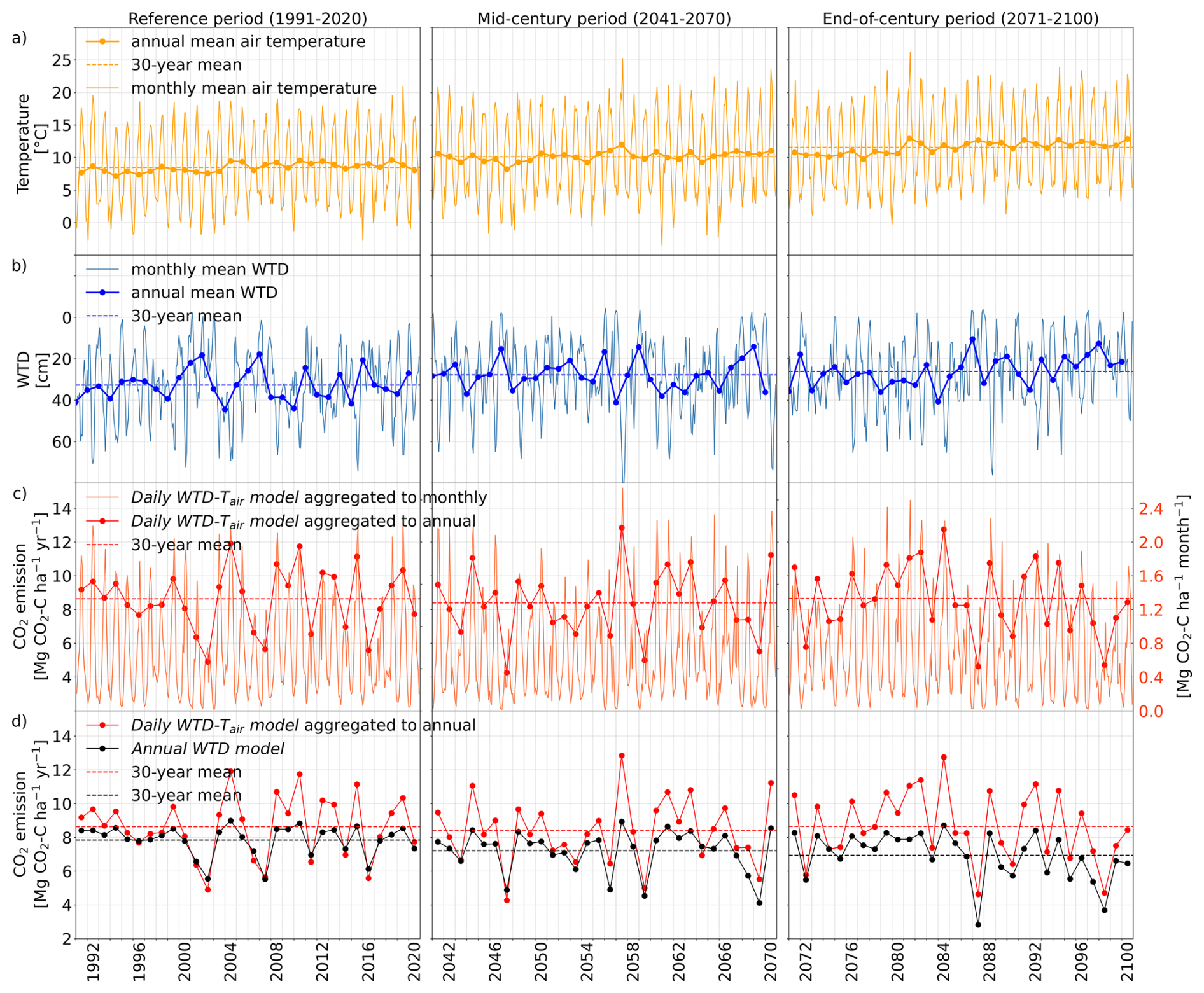
Figure 8 Example of air temperature (T_air), water table depth (WTD) and soil CO₂ flux for future climate simulation with climate model projection no. 5 (Table S6).

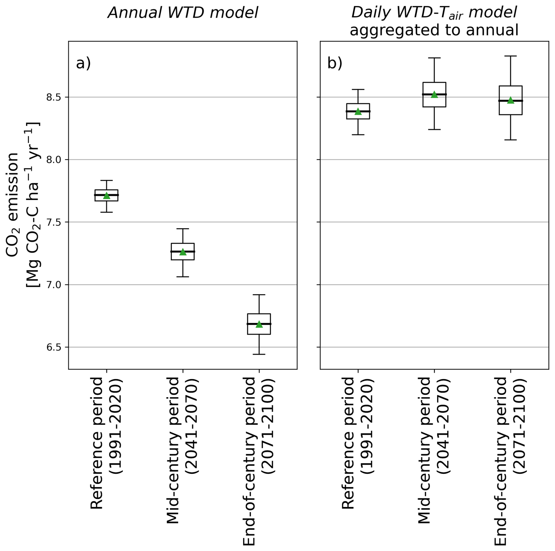
Figure 9 Boxplot showing the distribution of bootstrap means of soil CO₂ emissions according to the Daily WTD-T_air model and Annual WTD model during future climate. Green triangles and horizontal lines indicate the mean and the median of the bootstrap mean, respectively. Boxes show the 25th and 75th percentiles. Whiskers indicate the 95 % confidence intervals. Outliers are not shown.

The results presented in Fig. 9 suggest that the impact on CO₂ emissions caused by future increases in T_air and increases in water tables cancel each other out when using the Daily WTD-T_air model. To investigate this further, we analyze how the combination of T_air and WTD shift between the reference and the end-of-century periods, despite relatively stable total CO₂ emission.

We wish to identify the specific combination of T_air and WTD that are associated with the majority of the CO₂ emission. Due to the non-linear response of soil CO₂ flux to environmental drivers in the Daily WTD-T_air model, a large fraction of total emissions is generated on relatively few days. To quantify this, we calculated p50, defined as the proportion of days required to account for 50 % of the total annual soil CO₂ flux (fCO₂). This was achieved by ranking the daily values of fCO₂, WTD, and T_air in ascending order according to fCO₂. Subsequently, the ranked fCO₂ values were cumulatively summed to obtain their percentile distribution (Fig. S8). The procedure was first applied to fCO₂, WTD, and T_air data from the historical simulation period, with the resulting percentile curves shown in Fig. S8. Over the historical simulation period, 50 % of the total fCO₂ (fCO_2, p50) was generated within 22 % of the days (p50 = 22 %), while the value of fCO_2, p50 and corresponding WTD_p50 and T_air, p50 are estimated to be 4.15 × 10⁻² g CO₂-C ha⁻¹ d⁻¹, 47 cm and 13.8 °C (Table 6 and Fig. S8).

Similar estimates are derived from the three timeslots from the climate models (reference, mid-century and end-of-century climate simulation periods) using the 17 different climate models. For the future, 50 % of the total fCO₂ is expected to occur within approximately 21 ± 1 % (mean ± SD, n=17) of the days (Table 6). The daily soil CO₂ flux associated to p50 (fCO_2, p50) and p50 are nearly identical across both the historical and future climate simulations periods (Table 6). As also shown in Fig. 9b, the magnitude and temporal distribution of fCO₂ are predicted to remain unchanged in the future. While the value of fCO_2, p50 remains relatively constant around 4 × 10⁻² Mg CO₂-C ha⁻¹ d⁻¹ for future climate periods, the corresponding WTD_p50 and T_air, p50 values change as a result of changing climate moving towards higher temperatures (17 °C) and shallower groundwater table (40 cm) (Table 6).

Figure 10 provides a graphical representation of fCO₂ obtained from the Daily WTD-T_air model, with the colormap illustrating the daily fCO₂ corresponding to different combinations of T_air and WTD. The daily fCO_2, p50 (4.15 × 10⁻² g CO₂-C ha⁻¹ d⁻¹ for the historical period (Table 6)) can be achieved through various combinations of T_air and WTD (dark red dotted line in Fig. 10). The values of T_air, p50 and WTD_p50 corresponding to fCO_2, p50 for the Tuse Stream catchment peatland are plotted as a dark red point. As expected, the fCO_2, p50 values for the reference periods of the 17 climate models (green crosses at Fig. 10) are closely aligned with that of the historical period. It is evident that the fCO_2, p50 values for the end-of-century climate conditions (blue crosses at Fig. 10) shift along the direction indicated by the dark purple arrow (along the red dotted line), reflecting a trend toward higher temperatures and lower WTD (i.e. water levels closer to the surface surface). This indicates that the mean daily fCO₂ (Table 6) and the long-term fCO₂ remains constant in the future (Fig. 9b), as a result of a counterbalance between impacts of rising temperatures and rising groundwater levels.

The dark purple arrow at Fig. 10 illustrates the characteristic impact of climate change in Denmark, reflecting the concurrent increase in air temperature and shallow groundwater levels (Schneider et al., 2022). In contrast, other regions in Europe are experiencing declining groundwater level trends to climate change (Wunsch et al., 2022). Consequently, CO₂ emissions from peatlands in these regions are expected to shift in the direction indicated by the yellow arrow in Fig. 10, towards considerably larger emission rates.

Table 6 p50 is the fraction of days required to reach 50 % of the total soil CO₂ flux (fCO₂). fCO_2, p50 is the daily soil CO₂ flux associated with p50. WTD_p50 and T_air, p50 are the water table depth (WTD) and air temperature (T_air) corresponding to fCO_2, p50, respectively. Mean ± SD is based on 17 climate model simulations.

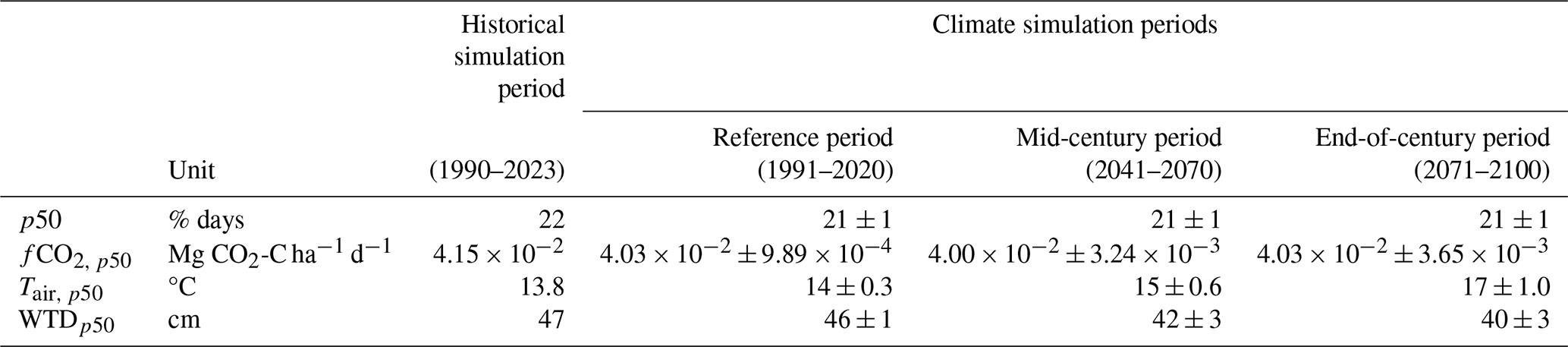
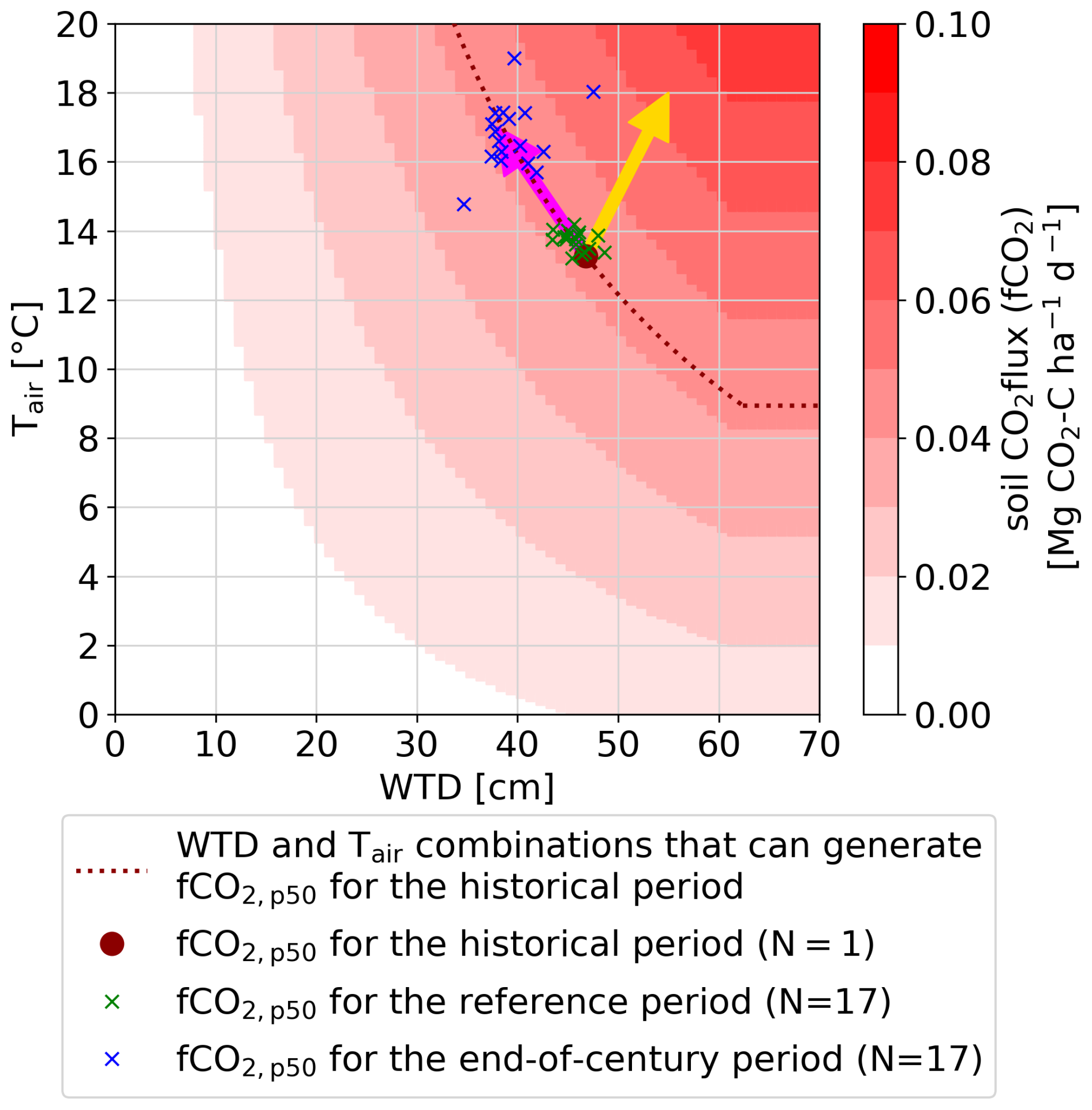
Figure 10 Colormap: Visual representation of the Daily WTD-T_air model output, illustrating soil CO₂ flux (fCO₂) as function of daily water table depth (WTD) and air temperature (T_air). The dark red dotted line represents combinations of T_air and WTD that corresponds fCO₂ at p50 (fCO_2, p50), where p50 is the fraction of days required to reach 50 % of the total accumulated fCO₂ during the historical period. Green crosses are fCO_2, p50 for the reference period of the 17 climate simulations. Purple crosses are fCO_2, p50 for the end-of-century climate simulation period of the 17 climate simulations. The pink and yellow arrows indicate different future trends in T_air and WTD and the associated trend in CO₂ emissions under climate change. Specific to Denmark, the pink arrow indicates increases in T_air and decrease in WTD, other regions might experience increase in both T_air and WTD and an associated large increase in CO₂ emissions (yellow arrow).

4 Discussion

4.1 Peatland management under changing climate

In 2023, CO₂ emissions from drained organic soils in croplands and grasslands was estimated to have accounted for 6.7 % of Denmark's total emissions, including those from the Land Use, Land-Use Change and Forestry (LULUCF) sector (Nielsen et al., 2025). Returning peatland organic soils to their natural hydrological state is a cost-effective GHG reduction strategy (IPCC, 2014; Kirpotin et al., 2021; Tanneberger et al., 2021; Wilson et al., 2016). Therefore, national policies (Regeringen, 2024) and the European Union's Nature Restoration Law seek to improve the management of peatlands and achieve climate neutrality targets under the urgent Green Transition agenda. To mitigate agricultural GHG emissions Danish ministerial agreements were initiated in 2024, targeting the restoration of 140 000 ha of peatland. Moreover, a CO₂ eq tax on emissions from organic peatlands is scheduled for implementation in Denmark from 2028 (Regeringen, 2024). However, there is a need to strengthen the scientific evidence for mitigation measures to facilitate cost-effective policies.

Integration of the process-based hydrological model of the Tuse Stream catchment with the empirically derived Daily WTD-T_air model of soil CO₂ flux developed in this study revealed that emission simulations at daily timesteps produce greater variability in soil CO₂ fluxes compared to emission estimates derived from annual WTD means. This increased variability is attributed to the daily model's ability to account for short-term compound events, especially the simultaneous occurrence of elevated air temperatures and low groundwater levels.

More importantly, incorporating temperature dependence and higher temporal resolution into the CO₂ emissions model significantly alters the projected trends of CO₂ emission under both rewetting and changing climate conditions.

Nature-based approaches represent the most common real-world rewetting strategies, aiming to restore peatlands towards their natural hydrological regime. At a minimum, such rewetting requires terminating tillage activities and eliminating artificial drainage for instance by blocking of drainpipes and ditches. The rewetting scenarios implemented in this study, represented as simple modifications to WTD, are not reflective of practical management interventions – except perhaps in a few rare and costly restoration projects that involve installing artificial impermeable membranes along peatlands edges (Naturstyrelsen, 2022). However, the outcome of this study can inform discussions on requirements and best practices for rewetting and peatland restoration. The study also highlights the need to monitor or model pre- and post-restoration WTD dynamics in order to develop realistic expectations regarding CO₂ emission reductions from rewetted peatlands.

The rewetting analyzed in this study showed how different rewetting scenarios with varying seasonal amplitudes in WTD suggest significantly different emission reduction potential even with identical annual mean WTD. The results illustrate that increasing the groundwater table during warm periods is key to obtaining CO₂ emission reductions, whereas rewetting strategies that mainly raise winter water table without significantly affecting the summer levels offer limited mitigation benefits. This highlights the importance of not only targeting annual reductions in WTD but particularly designing rewetting strategies to increase the summer water table and avoid critically low water levels during droughts and warm periods. Achieving such rewetted conditions may include larger forced control of WTD than what is currently being practiced for most existing rewetting schemes, where the WTD remain subject to climate seasonality impact. Such nature-based solutions are not likely to reduce CO₂ emissions to the degree that current emission reduction policies target. Also, projections of CO₂ emissions under different climate change scenarios were altered greatly by introducing temperature sensitivity and enhanced temporal resolution into the CO₂ emissions modeling framework. Here our results show that, while the projected rise in groundwater tables in isolation would lead to lower CO₂ emissions in future (when using the Annual WTD model), the Daily WTD-T_air model revealed that anticipated increases in T_air are likely to cancel out these reductions, resulting in CO₂ emissions on a level comparable to current levels. This is an important finding, since it suggests that increasing temperatures alone will likely increase CO₂ emissions, and that water level rise driven by climate change or rewetting initiatives might just counteract this trend. Rewetting measures would need to be substantially intensified to ensure climate resilience and achieve meaningful reductions in CO₂ emissions. Additionally, outside the specific case of Danish peatlands located in a region that is susceptible to a future wetter climate, other regions might project both increasing temperatures and lower groundwater tables, and in such cases climate change will significantly increase emissions without any rewetting. We acknowledge that the chosen RCP8.5 represents the scenario leading to the strongest impact of climate change and that additional, milder climate scenarios could have been included.

4.2 Hydrological simulation of groundwater levels in peat soil with process-based models

Existing large scale CO₂ emission estimates, such as national inventories from organic soils (Gyldenkærne et al., 2025; Nielsen et al., 2025), typically combine empirical emission models and data-driven ML approaches for estimating annual WTD (Bechtold et al., 2014; Koch et al., 2023; Tiemeyer et al., 2020). These approaches appear robust and suited for upscaling but are limited in their ability to represent the impact of sub-annual variability in temperature and WTD, which are issues that become increasingly important when analyzing effects of rewetting and climate change. In contrast to most data-driven approaches, hydrological models enable a climate-driven representation of WTD temporal dynamics and the underlying hydrological processes. Moreover, the use of physically based hydrological models has the distinct advantage of enabling scenario-based analyses, such as the evaluation of alternative land use strategies and the projection of future hydrological conditions under climate change scenarios. Utilizing hydrological models that generate high-resolution time series of WTD, it is possible to quantify impacts of WTD dynamics, including water levels, temporal variability and seasonal amplitudes, on changes in CO₂ emissions.

That said we acknowledge that the rewetting scenarios in the present study are applied using simplified adjustments to the simulated WTD, rather than being modeled through a detailed, process-based hydrological framework. Ideally, future assessments should apply catchment-scale models to evaluate peatland management interventions, such as rewetting, thereby enabling analysis of their broader hydrological impacts, including effects on streamflow and groundwater levels in neighboring areas. A unique feature of the present study is that the hydrological model of Tuse Stream catchment is developed in the same modelling framework as the National Hydrological Model of Denmark (Henriksen et al., 2020; Stisen et al., 2019). The National Hydrological Model is continuously updated with new data and operates in near real-time. This integration enables a link between the lessons learned from the Tuse Stream catchment-scale model and the National Hydrological Model of Denmark, thereby improving the representation of peatland hydrology and contributing to the refinement of future national GHG inventories.

As a continuation of this study, we will further investigate the spatial variability of WTD and extent hydrological model to include additional peatland-dominated catchments. Additionally, we will utilize the National Hydrological model to simulate WTD across all Danish peatlands.

4.3 Selection, fit and transferability of daily CO₂ emission model

Detailed process-based terrestrial ecosystem models that simulate biogeochemical cycles and vegetation are available (Bona et al., 2020; Oikawa et al., 2017; Wu and Blodau, 2013). Such modelling schemes rely largely on multiple parameters related to plant and soil biogeochemistry which are not generally attainable, thereby limiting the possibility to generalize and upscale.

As an alternative a range of empirical models with varying levels of complexity has been developed to describe ecosystem respiration; however, the most commonly applied formulation is the Lloyd–Taylor model (Lloyd and Taylor, 1994), in which temperature acts as the sole independent variable. Structural complexity in empirical equations is increased through the integration of various other environmental variables, for example, hydrological variables such as WTD (Rigney et al., 2018). Recent alternative empirical approaches for estimating CO₂ emissions for organics soils include response functions linking average annual WTD to annual emissions (Arents et al., 2018; Evans et al., 2021; Tiemeyer et al., 2020), such as the Annual WTD model (Koch et al., 2023) used in this study.

To evaluate alternative empirical emission models alongside our Daily WTD-T_air model, we fitted three different empirical formulations from Rigney et al. (2018) to the Vejrumbro soil CO₂ flux data (Table S7). Each of the three empirical formulations incorporated both temperature and WTD as independent variable. The model fitting resulted in R² values comparable to those obtained from fitting the Daily WTD-T_air model developed in this study (Table S7).

Studying the explanatory power of each independent variable of WTD and T_air in isolation in the other empirical emission models, revealed that models in which WTD and T_air are incorporated as additive terms, rather than as interdependent (e.g., multiplicative) terms (as in Eqs. 6 and 8 in Rigney et al., 2018), often exhibit coefficients of determination (R²) that are excessively dominated by either WTD or T_air (Table S7). This indicates that such model formulations may inadequately capture the joint or synergistic effects of these variables on the dependent variable. The challenge likely stems from the fact that both WTD and T_air exhibit similar seasonal patterns, which may lead the regression to primarily fit one of the additive terms containing either WTD or T_air. Empirical models that incorporate WTD and T_air as multiplicative terms (such as Eq. 7 in Rigney et al., 2018, and the Daily WTD-T_air model developed in this study) demonstrate a more balanced distribution of explanatory power between each independent variable (Table S7). Nevertheless, Eq. (7) in Rigney et al. (2018) remains predominantly influenced by the T_air component (Table S7). A more balanced distribution of explanatory power between temperature and WTD is desirable, given that both variables are recognized as key drivers of soil CO₂ flux dynamics, which is achieved better with the Daily WTD-T_air model than with any of the empirical models in Table S7.

We acknowledge that the Daily WTD-T_air model does not reproduce many of the highest observed fCO₂ values (Figs. S6 and S7). In addition to identifying a relationship between fCO₂ and WTD, which was used to derive the Daily WTD-T_air model (Fig. S5), we studied the temperature sensitivity within WTD bins to better understand the model's inability to reproduce the highest observed fCO₂ values. Specifically, we binned the daily fCO₂ into four WTD intervals: < 20 cm (n=73), 20 to 40 cm (n=37), 30 to 40 cm (n=77) and > 40 cm (n=44) (Fig. S9). We identified a potential relationship between fCO₂ and temperature within WTD bins (Fig. S9). This result is expected given the strong interdependence among fCO₂, temperature and WTD, all of which exhibit comparable seasonal dynamics. The high observed fCO₂ values cannot be captured by a simple empirical model based solely on T_air and WTD, particularly because both high and low fCO₂ occur under similar T_air and WTD conditions (Figs. S5, S7 and S9). Consequently, the Daily WTD-T_air model represents a compromise that captures part of the variability while preserving a realistic mean response.

In this study, we demonstrate the need for the development of emission models operating on a sub-annual timescale. It highlights the necessity of creating scalable generalized models based on temperature, WTD and possibly other predictors. The development of such models requires data from a large number of sites with continuous and temporally dense measurement, in order to integrate information in a manner similar to models based on annual WTD. We recognize that currently, models based on annual WTD are likely the most robust for upscaling to national level and current conditions.

The simulated soil CO₂ flux at Vejrumbro, estimated using the Daily WTD-T_air model (13.6 Mg CO₂-C ha⁻¹ yr⁻¹), aligns well with flux measurements from Danish and German sites (Fig. 5). This agreement suggests a comparable magnitude of emissions across geographically distinct locations of similar characteristics, such as soil type and land use history.

We acknowledge that the Daily WTD-T_air model is derived from a single dataset, and that other emission models also provide valid fits of WTD and T_air. Furthermore, we recognize that empirical emission models are highly dependent on the specific data to which they are fitted. Acknowledging the limited data behind the Daily WTD-T_air model utilized in this study, the goal has not been to accurately estimate the peatland emission budget, which will be uncertain due to the reliance on a single site. However, the objective has been to illustrate the impact and insights gained from applying emission models at a daily timescale and how this has significant impact on the conclusions that can be made regarding effects of rewetting and climate change. The decision to utilize the Daily WTD-T_air model for rewetting and climate modeling scenarios is motivated by the simplicity of the relationship and its direct derivation from the Vejrumbro data, which clearly demonstrates a temperature-dependent relationship between soil CO₂ flux and WTD. The limited availability of multiple high-temporal-resolution GHG emission datasets broadly restricts the ability to generalize and upscale empirical GHG emission models at a daily timescale. Therefore, we consider the Daily WTD-T_air model to be the most reliable option currently available. Future research should validate the performance of emission models on intra-annual (within years) data with continuous measured CO₂ data.

A promising methodology for future applications, as well as for integrating a Tier 3 framework, involves coupling a process-based hydrological model with process-based emission models or an empirically derived daily emission model, such as the one developed in this study, to enable detailed simulations of GHG emissions that capture short-term dynamics and compound environmental effects.

5 Conclusions

This study demonstrates the feasibility of simulating the temporal dynamics of the peatland water balance and shallow groundwater table depth (WTD) using a catchment-scale distributed hydrological model. Accurately modelling shallow WTD is critical for reliable projections of CO₂ emissions from peatlands. We combined simulations of shallow WTD from the calibrated hydrological model with two empirical CO₂ emission models (1) an annual WTD-CO₂ relationship and (2) a daily WTD-CO₂ model accounting for the temperature effect on soil CO₂ production. This approach was used to estimate net soil CO₂ emissions for the historical period (1991–2020), the mid-century period (2041–2070) and the end-of-century period (2071–2100). This demonstrated that projections of soil CO₂ emissions are highly sensitive to the complexity and temporal resolution of the emission model applied. Specifically, models that incorporate both temperature and WTD dynamics at a daily timescale results in vastly different conclusion regarding impacts of climate change and rewetting. Regarding climate change impacts, we show that a daily temperature and WTD based emission model predict increased emissions due to temperature changes, which can be counter balanced (in the Danish case) or amplified depending on the future trend in WTD. Our results also demonstrate that rewetting strategies aimed at raising the groundwater table during the warm summer period offer a CO₂ emission reduction potential of up to 50 %, whereas approaches focused primarily on increasing winter water table levels result in only marginal reductions. The combination of process-based hydrological model simulations and a daily-resolution empirical CO₂ emission model used in this study captures the influence of short-term compound climate events – such as simultaneous high temperatures and low WTD – which substantially alters projected emission trends compared to simpler approaches. Such refined approaches are essential for developing adaptive, climate-resilient peatland restoration policies and improving national greenhouse gas inventories. The findings underscore the importance of moving beyond static, annual WTD thresholds in peatland management by incorporating dynamic hydrological simulations. Instead, rewetting strategies should prioritize maintaining elevated summer groundwater table levels to buffer against drought-induced emission peaks.