Substantial inter-model variation in OAE efficiency between the CESM2/MARBL and ECCO-Darwin ocean biogeochemistry models

Induction of a CO₂ partial pressure (pCO₂) deficit in the surface-ocean through ocean alkalinity enhancement (OAE) or direct ocean removal (DOR) methods has been recognized as a promising approach to meet the projected need for negative CO₂ emissions. The difficulty of directly measuring the counterfactual CO₂ flux due to rapid spreading of the DIC-deficient plume has put ocean circulation models in the center of the Measurement, Reporting and Verification (MRV) challenge. Confidence in the results of such models is essential for the emerging industry to access carbon credit markets and grow at the required pace, to reach substantial negative emissions by 2050, as envisioned by the Intergovernmental Panel on Climate Change (IPCC).

The kinetics and equilibration time of such a DIC deficit have been shown to vary substantially depending on the location and season of the initial induction point. A major component of this variance is the vertical transport and mixing of the DIC-deficient plume; however, air-sea CO₂ gas exchange and carbonate chemistry are also important.

Currently, it is poorly understood how much the results of OAE pulse simulations depend on the models chosen. To help close this knowledge gap, we investigate two global circulation models, the CESM2/MARBL model (1°) and the data-assimilative ECCO-Darwin model ($\mathrm{1}/\mathrm{3}$°). We perform pulse injection simulations at twelve locations with both models, matched precisely in terms of injection patch geometry, release year and season. We analyze the differences in CO₂ uptake curves, vertical mixing, gas exchange and carbonate chemistry.

We show that in some locations, such as subtropical regions, substantial differences exist between these two models – well beyond the expected intrinsic variation of each model. Furthermore, we demonstrate that the majority of the differences are attributable to the representation of vertical transport, especially mixed layer depth, followed by the effect of wind parameterizations; a small amount of difference is attributable to carbonate chemistry parameterization. In some locations, there exists good agreement between the models. In most injection locations, the largest differences between models are found in the first 7 years post alkalinity injection; in many this is followed by slow convergence towards the expected theoretical maximums.

1 Introduction

Marine Carbon Dioxide Removal (mCDR) methods (Press, 2022; Oschlies et al., 2023; Renforth and Henderson, 2017) have recently gained significant attention as a scalable set of approaches to achieve the magnitude of negative emissions called for by IPCC models to keep global-mean temperature change below 2 °C by 2100 (Rogelj et al., 2018; Metz and Intergovernmental Panel on Climate Change, 2005; IPCC, 2021; Rickels et al., 2018). These methods work by inducing a pCO₂ deficit in the surface ocean, which causes excess CO₂ uptake by the ocean. The word excess here is used to indicate the excess relative to a counterfactual scenario without the intervention. The pCO₂ deficit can be created in a variety of ways. The removal of CO₂ from surface waters (Direct Ocean Removal, DOR) and subsequent storage of CO₂ in geological reservoirs or the cultivation of macroalgae followed by removal or sinking of plant matter both remove dissolved inorganic carbon (DIC) from surface waters. Alternatively, the dissolution of alkaline materials in surface water or the removal of acidity through electrochemical means also lead to a DIC deficit by altering the carbonate equilibrium (Oschlies et al., 2023; Renforth and Henderson, 2017).

In both situations, however, the induction of the pCO₂ deficit does not immediately remove CO₂ from the atmosphere (Broecker and Peng, 1982). Instead, this process occurs on the order of years or decades, depending on the speed of gas exchange and the residence time of surface waters (Jones et al., 2014; Wang et al., 2023; Suselj et al., 2025). Previous work has shown a complex dependency on the release location as the DIC deficient plume spreads across entire ocean basins over the timescale of equilibration, with subduction processes removing the deficit from contact with atmosphere while also potentially transporting it later into surface waters elsewhere (He and Tyka, 2023; Suselj et al., 2025; Zhou et al., 2025).

The geographical region over which ocean dynamics contribute to the equilibration process is so large that direct experimental measurement of the counterfactual CO₂ uptake would be extremely difficult in practice (Mace et al., 2021; Subhas et al., 2025) considering that the dilution of the plume leads to sub-µatm changes in surface pCO₂ (He and Tyka, 2023), which are very difficult to measure (Wanninkhof et al., 2013). Furthermore, the counterfactual values of surface pCO₂ are inaccessible to direct measurement and changes in pCO₂ are difficult to attribute if multiple OAE deployments exhibit spatial overlap in their alkalinity plumes (He and Tyka, 2023). Therefore, the Measurement, Reporting and Verification (MRV) of mCDR efforts will likely lean heavily on ocean modelling efforts (Bach et al., 2023; Fennel et al., 2023; Fennel, 2025).

Recently, an extensive map of Ocean Alkalinity Enhancement (OAE) equilibration curves, covering multiple seasons, was calculated using the CESM2/MARBL general circulation model (GCM) (Zhou et al., 2025) and strong seasonal and regional variation was identified. Yankovsky et al. (2025) extended the work to investigate interannual variability, which is inherent to any given model, and found some regions exhibit substantial variation of uptake rates from year to year, owing to differences in circulation patterns. However, to date, the inherent model uncertainty or confidence relative to other models is largely unknown. Previous efforts have compared different circulation or Earth System Models (ESMs) and the variance in their predictions (Keller et al., 2018), but specifically how their differences influence the OAE equilibration curves has not been explored. Xie et al. (2025) recently investigated the effect of different horizontal grid resolutions and found comparatively small differences across different resolutions of the same model, noting that the resolutions spanned 0.1° to 1° and at best only resolved mesoscale dynamics, yet identified large differences when comparing entirely different models. We therefore focus our attention to comparing two models side-by-side (the aforementioned CESM2/MARBL GCM and the ECCO-Darwin model) using pulse injections of surface-ocean alkalinity. Our goal is to examine not only the extent of the variability but to pinpoint the components of the model set-ups or parameterizations which make the largest difference to the equilibration curves.

2 Methods

2.1 Ocean models

Using the polygonal subdivision of the ocean introduced in Zhou et al. (2025), we selected 12 locations, spanning the range of the four different OAE uptake regimes identified by Zhou et al. (2025). The locations chosen are shown in Fig. 1 and listed in Table S1.

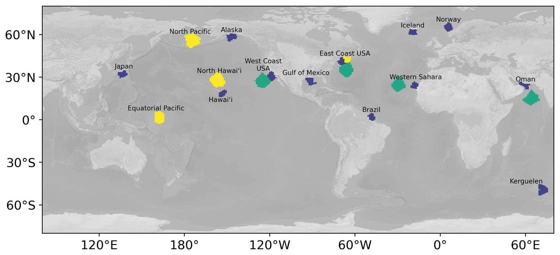
Figure 1 Locations selected for inter-model comparison. The twelve main locations investigated here are shown in blue. In four cases (green) a nearby area further offshore was also examined. In yellow are shown four locations from Yankovsky et al. (2025), which were compared to equivalent injection years in ECCO-Darwin. See also Tables S1 and S2.

Since the ECCO-Darwin model uses a different grid (so-called Lat-Lon-Cap, (LLC270)) grid at $\mathrm{1}/\mathrm{3}$° (Zhang et al., 2018)) compared to the CESM2/MARBL model (1° spherical-polar grid), we re-projected the polygonal subdivisions (Zhou et al., 2025) onto the finer, $\mathrm{1}/\mathrm{3}$° LLC270 grid. While the difference in gridding means that the release locations cannot be exactly replicated, the difference in the release area boundaries is very small and not expected to significantly alter the uptake curves. This assumption is supported by the observation that the CO₂ uptake curves obtained previously vary across the ocean only gradually (Zhou et al., 2025). In each location, alkalinity was released over the period of one month (in January) at a rate of 10 mol m⁻² yr⁻¹ uniformly across the selected polygon.

We conducted each of the pulsed alkalinity simulations using the standard LLC270 ECCO-Darwin $\mathrm{1}/\mathrm{3}$° model set-up for 15 years (Zhang et al., 2018; Carroll et al., 2020, 2022, 2024). For each location, we investigated two pulses, one in 1992 and one in 1999 in two separate simulations. The latter matches the exact release year used in Zhou et al. (2025) while the former provides an indication of the interannual variability. The year 1992 was not chosen for any particular climatological reasons, but rather, being the earliest year in ECCO-Darwin's data assimilative period, allows for potentially the longest continuous simulation. The atmospheric concentration of CO₂ was set to historical values from the NOAA Greenhouse Gas Marine Boundary Layer Reference (Andrews et al., 2014). Small differences in pCO${}_{\mathrm{2}}^{\mathrm{atm}}$ are not expected to change the OAE uptake curves, so long as the value is not responsive to induced CO₂ uptake (Tyka, 2025). The total volume-integrated amount of ocean DIC was then computed over the simulation period and the difference from a reference counterfactual simulation was obtained. This was then normalized by the total amount of alkalinity added initially to yield $\mathit{\eta }\left(t\right)=\mathrm{\Delta }\mathrm{\Sigma }\mathrm{DIC}\left(t\right)/\mathrm{\Delta }\mathrm{\Sigma }\mathrm{Alk}$ as the metric of OAE efficiency (Zhou et al., 2025), where the sums are over the entire ocean volume.

In the same way as described above, we also tested four additional locations (North Pacific, North Hawai'i, Equatorial Pacific and Gulf Stream) replicating exactly the experiments of Yankovsky et al. (2025). Here, 5 runs were conducted for 5 years each, with alkalinity addition pulses in January of 2000, 2003, 2006, 2009 and 2012, with the goal of quantifying interannual variability.

2.2 CESM2/MARBL

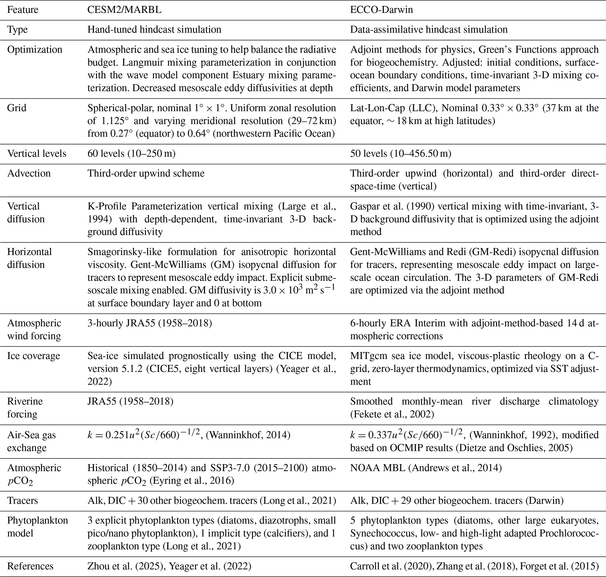
The CESM2/MARBL model configuration used in this study is described in detail in Zhou et al. (2025) and references therein. Briefly, the CESM2/MARBL simulation is a global forced ocean-ice (FOSI) configuration (Yeager et al., 2022) of the Community Earth System Model v.2 (CESM2) (Danabasoglu et al., 2020). The ocean component is the Parallel Ocean Program v.2 (POP2) with nominal horizontal resolution of 1° × 1° and biogeochemistry simulated by MARBL (Long et al., 2021). The model was forced with the Japanese 55-year atmospheric reanalysis dataset (JRA55) (Kobayashi et al., 2015; Tsujino et al., 2018), spun up from 1850 to 2019. The simulation is not data constrained, and all simulations in this study were forced with historical atmospheric CO₂. Further properties and features of the model are summarized in Table 1.

2.3 ECCO-Darwin

A detailed description of the ECCO-Darwin model set-up, observational constraints, optimization methodology, and model-data evaluation is presented in Carroll et al. (2020, 2022, 2024). The latest ECCO-Darwin solution (v05) used here is based on ocean circulation and physical tracers (i.e., temperature, salinity, and sea ice) from the Estimating the Circulation and Climate of the Ocean (ECCO) LLC270 global-ocean and sea-ice data synthesis (Zhang et al., 2018). ECCO-Darwin is based on a global-ocean and sea-ice configuration of the Massachusetts Institute of Technology general circulation model (MITgcm) (Marshall et al., 1997), which has been constrained by the ECCO project using nearly all available ocean observations for the 1992–near-present period and has horizontal grid spacing of $\mathrm{1}/\mathrm{3}$° at the equator and ∼ 18 km at high latitudes, with 50 vertical levels. It should be noted that this configuration uses the ECCO LLC270 grid, which is a higher-resolution variant distinct from the more commonly used LLC90 production version (Forget et al., 2015). The ECCO circulation estimate is coupled online with the MIT Darwin ocean ecosystem model, which in turn drives and interacts with marine chemistry and ocean carbon variables (Dutkiewicz et al., 2015), providing a data-constrained, property-conserving estimate of the three-dimensional, time-evolving ocean, sea ice, biogeochemical, and ecological state. An extensive global-ocean evaluation of v05 ECCO-Darwin against in-situ data is provided in Carroll et al. (2024). The ECCO-Darwin ecology includes five phytoplankton function types (diatoms, other large eukaryotes, Synechococcus, and low- and high-light adapted Prochlorococcus) and two zooplankton types with different preferential grazing behavior (Brix et al., 2015). The biological rates are driven by light, temperature, and macro/micronutrients (nitrogen, phosphorus, iron, and silica) but do not explicitly depend on DIC and Alk. Conversely the circulation does not depend on the tracers.

The optimization method of ECCO-Darwin uses the adjoint method for the physics, which adjusts initial conditions, surface-ocean boundary conditions, and 3-D time-invariant mixing coefficients; model biogeochemistry is optimized using a low-dimensional Green's Functions approach to adjust initial conditions and Darwin parameters. This results in a physically-consistent counterfactual solution with fully-closed property budgets (i.e., no nudging is used in the assimilation process). We note that ECCO-Darwin does not have a long spin-up period from pre-industrial conditions, as done in many forward-only ocean and Earth System Models, but uses the ECCO data assimilation methodology to both reduce spin-up and drift in a data-constrained simulation that starts in 1992. Table 1 summarizes the main features and parameterizations for both models.

(Large et al., 1994)Gaspar et al. (1990)(Yeager et al., 2022)(Fekete et al., 2002)(Wanninkhof, 2014)(Wanninkhof, 1992)(Dietze and Oschlies, 2005)(Eyring et al., 2016)(Andrews et al., 2014)(Long et al., 2021)Zhou et al. (2025)Yeager et al. (2022)Carroll et al. (2020)Zhang et al. (2018)Forget et al. (2015)

Table 1 Side by side comparison of the two biogeochemical models used in this study.

2.4 Overall inter-model differences

In addition to quantifying the empirical differences in OAE-induced CO₂ uptake between different ocean models, the goal of this paper is to estimate the relative importance of different model aspects to the overall variance. A better understanding of these sources of discrepancy will inform future model development and potentially inspire new sources of model-constraining data collection.

The main aspects of the ocean models which conceivably contribute to the CO₂ equilibration dynamics are: horizontal and vertical transport (advection and mixing) of the excess alkalinity plume, the gas transfer velocities (which are a function of wind speed and sea-ice cover), the carbonate chemistry parameterization and any biological processes which can affect DIC or alkalinity concentrations. These aspects are strongly intertwined; for example, changes in horizontal transport will affect plume dispersal and therefore which gas transfer velocities will be encountered by the space-time evolving trajectory of the plume. Similarly temperature and salinity can affect the carbonate chemistry state and hence pCO₂.

We first compare these aspects in a generic way, comparing the wind forcing and carbonate parameters as function of latitude, longitude and time. These comparisons help identify overall differences in parameterization and are not specific to any given injection location. We then conduct a deeper analysis which compares the influence of each parameter to any given release location and alkalinity plume.

2.4.1 Carbonate parameters

As a further reference point we also compared both models' carbonate parameters to a data-based product. Experimental data for global surface-ocean alkalinity (Alk), DIC and pCO₂ were obtained from OceanSODA (Gregor and Gruber, 2021). The simulations with CESM2/MARBL and ECCO-Darwin also generated monthly-mean [Alk] and [DIC] fields throughout the simulation (where the square brackets mean “concentration of”). For analysis and comparison purposes, the ECCO-Darwin and CESM2/MARBL fields were regridded onto the OceanSODA grid, using nearest neighbor interpolation.

For the latitudinal comparison of carbonate parameters (Fig. 10) the Mediterranean Sea was excluded. Based on values of surface-ocean [Alk] and [DIC], as well as salinity, temperature and concentrations of borate, phosphate and silica, the full surface-ocean carbonate system was solved offline using PyCO2SYS (Humphreys et al., 2020) at monthly intervals, yielding values for [CO₂], $\left[{\mathrm{HCO}}_{\mathrm{3}}^{-}\right]$ and $\left[{\mathrm{CO}}_{\mathrm{3}}^{\mathrm{2}-}\right]$ (Note that throughout this paper, the [CO₂] includes both dissolved CO₂ and undissociated carbonic acid H₂CO₃ following the convention used by Zeebe and Wolf-Gladrow, 2001). The quantity ${\mathit{\eta }}_{\max }=\partial \left[\mathrm{DIC}\right]/\partial \left[\mathrm{Alk}\right]$ was calculated using the exact equation (for derivation see Supplement and Humphreys et al., 2018)

$$\begin{array}{}\text{(1)}& {\displaystyle \frac{\partial \left[\mathrm{DIC}\right]}{\partial \left[\mathrm{Alk}\right]}}={\displaystyle \frac{\left[{\mathrm{HCO}}_{\mathrm{3}}^{-}\right]+\mathrm{2}\left[{\mathrm{CO}}_{\mathrm{3}}^{\mathrm{2}-}\right]}{\begin{array}{c}\left[{\mathrm{HCO}}_{\mathrm{3}}^{-}\right]+\mathrm{4}\left[{\mathrm{CO}}_{\mathrm{3}}^{\mathrm{2}-}\right]+\left[{\mathrm{OH}}^{-}\right]+\left[{\mathrm{H}}^{+}\right]\\ +\left[B\right(\mathrm{OH}{)}_{\mathrm{4}}^{-}\left]\right[B\left(\mathrm{OH}{)}_{\mathrm{3}}\right]/B_{\mathrm{T}}\end{array}}}\end{array}$$

where B_T is the total borate concentration. The unitless carbonate sensitivity $\partial \left[\mathrm{DIC}\right]/\partial \left[{\mathrm{CO}}_{\mathrm{2}}\right]$ was, likewise, calculated using an exact equation (for derivation see Supplement):

$$\begin{array}{}\text{(2)}& {\displaystyle \frac{\partial \left[\mathrm{DIC}\right]}{\partial \left[{\mathrm{CO}}_{\mathrm{2}}\right]}}={\displaystyle \frac{\left[\mathrm{DIC}\right]}{\left[{\mathrm{CO}}_{\mathrm{2}}\right]}}-{\displaystyle \frac{\left(\right[{\mathrm{HCO}}_{\mathrm{3}}^{-}]+\mathrm{2}[{\mathrm{CO}}_{\mathrm{3}}^{\mathrm{2}-}\left]\right)}{\left[{\mathrm{CO}}_{\mathrm{2}}\right]}}{\displaystyle \frac{\partial \left[\mathrm{DIC}\right]}{\partial \left[\mathrm{Alk}\right]}}.\end{array}$$

2.5 Ablation of biological model

Another way to compare models is to conduct what is known in the machine learning community as “ablation”. Here, parts of a model are deliberately turned off or changed, and the simulations are repeated to examine their effects on the outcomes. We take this approach here with the biogeochemical model of ECCO-Darwin, which comprises 31 biogeochemical tracers, which, in addition to Alk and DIC, include Oxygen, Nitrate, Nitrite, Ammonia, Phosphate, Iron, Silica, Dissolved Organic Carbon and multiple phytoplankton functional type (PFT) tracers among others. These tracers are used to simulate biological activity, nutrient dynamics and carbonate precipitation and dissolution, in addition to inorganic processes such as gas exchange.

While biological processes modeled in ECCO-Darwin consume or produce CO₂ and/or Alkalinity (through carbonate shell creation or dissolution), the growth rates are not explicitly coupled to DIC or Alk. We therefore reasoned that the majority of the biogeochemical model should have very little, if any, influence on the CO₂ uptake curves, provided the background state of the DIC gradients (which biology helps establish) are present at the start of the simulation. If true, a significant fraction of computational cost could be saved in future simulations.

To test this hypothesis we created an ablated version of the ECCO-Darwin in which the marine ecosystem component was turned off in the code, i.e. an ocean without the soft tissue pump or calcifying activity. The only processes that remained active were the surface gas exchange, the advection of the tracers Alk and DIC, and the calculation of the carbonate system and pH. Alkalinity injections in eight different locations (plus an unperturbed reference run) were examined in this way, each with one run conducted with biological processes enabled and one run conducted without these features. Note that we did not spin up the system anew, or let the system reequilibrate into a new steady state which lacks the soft tissue pump and its associated DIC gradients before running the simulations. This was done intentionally to avoid changing the background carbonate state of the surface ocean, which would undoubtedly change the uptake kinetics. Instead, this experiment asks more narrowly: does the simulation of biological processes directly influence the CO₂ uptake curves over a short timescale (15 years)? The sudden loss of the biological pump at the beginning of the simulations causes a steady departure of DIC from the regular ECCO-Darwin trajectory; however, those changes are still relatively small over the 15-year model period, such that the background ocean state still corresponds well to the full ECCO-Darwin carbonate state (See Fig. S3).

2.6 Plume-specific intermodel differences

Thus far, our analysis has compared the parameter sets of the two models as a whole, however, for each release location the relative importance of various contributing factors to the CO₂ uptake will vary, depending on the trajectory of the spreading alkalinity plume. In this section we develop a framework which attempts to disambiguate, to an extent possible, different contributions in a plume-specific way.

Figure 2 Three different plume outlines overlaid on the k parameter in greyscale from OceanSODA(Gregor and Gruber, 2021). State is shown (a) 12 (b) 36 and (c) 72 months after alkalinity release near Alaska.

This is illustrated in Fig. 2 for an alkalinity release near Alaska. The extent of the alkalinity plume from three different runs is overlaid on the local gas-exchange parameter k. One can see how the intersection of the plume with k (as well as the other gas-exchange parameters) will determine the overall equilibration rate. Different models will not only have different gas-exchange parameters, they will also predict different plume trajectories – both contributing to the overall observed variance between models. The goal of the following section is to develop a framework to be able to attribute the differences to the various contributing aspects. The central idea is to reconstruct the equilibration rate of a given run (i.e. the gradient of the observed η(t) uptake curve) from the spatial extent of the plume at any given time t and the gas-exchange parameters that this plume is intersecting at that time. Then, an individual term in this expression may be swapped out to examine the sensitivity of the overall rate to that term. We develop this framework in the following section.

2.6.1 Rate expression for equilibration

In both ECCO-Darwin and CESM2/MARBL, the flux of CO₂ across the air-sea interface is modelled as proportional to the partial pressure difference for each surface grid cell

$$\begin{array}{}\text{(3)}& F_{{\mathrm{CO}}_{\mathrm{2}}}=k\mathit{\alpha }(p{\mathrm{CO}}_{\mathrm{2}}^{\mathrm{atm}}-p{\mathrm{CO}}_{\mathrm{2}}^{\mathrm{ocn}}),\end{array}$$

where α is the solubility of CO₂ in seawater (mol m⁻³ atm⁻¹) and k is the effective gas transfer velocity (m s⁻¹). Typically, k is parameterized as a function of wind speed squared k_w∝U² (Ho et al., 2006; Wanninkhof, 2014) and weighted by the sea-ice cover fraction α_ice, where it is assumed that complete sea-ice cover fully suppresses air-sea gas exchange.

$$\begin{array}{}\text{(4)}& k=(\mathrm{1}-{\mathit{\alpha }}_{\mathrm{ice}})k_{\mathrm{w}}\end{array}$$

The DIC concentration in the surface-ocean layer of the simulation (of thickness z₀ and volume V₀) then changes due to gas-exchange according to (Zhou et al., 2025; Zeebe and Wolf-Gladrow, 2001)

$$\begin{array}{}\text{(5)}& {\displaystyle \frac{\mathrm{d}}{\mathrm{d}t}}[\mathrm{DIC}{]}_{z=\mathrm{0}}=F_{{\mathrm{CO}}_{\mathrm{2}}}{\displaystyle \frac{A}{V_{\mathrm{0}}}}={\displaystyle \frac{k\mathit{\alpha }}{z_{\mathrm{0}}}}(p{\mathrm{CO}}_{\mathrm{2}}^{\mathrm{atm}}-p{\mathrm{CO}}_{\mathrm{2}}^{\mathrm{ocn}}),\end{array}$$

where A is the surface area over which the gas transfer occurs. Zhou et al. (2025) showed that this differential equation also applies to the difference between two simulations, the perturbed and reference simulation respectively, as performed in this work. Especially for small perturbations over which the carbonate system is linear, i.e. where $\mathit{\beta }=\partial \left[\mathrm{DIC}\right]/\partial \left[{\mathrm{CO}}_{\mathrm{2}}\right]$ is approximately constant, the induced change in DIC can be described using the following ordinary differential equation.

$$\begin{array}{}\text{(6)}& {\displaystyle \frac{\mathrm{d}}{\mathrm{d}t}}\mathrm{\Delta }[\mathrm{DIC}{]}_{z=\mathrm{0}}=-{\displaystyle \frac{k}{\mathit{\beta }{z}_{\mathrm{0}}}}\mathrm{\Delta }[\mathrm{DIC}{]}_{z=\mathrm{0}},\end{array}$$

where Δ[DIC] is the difference in DIC concentration between the reference and perturbed simulation. The factor β accounts for the fact that the effective capacity of the ocean for CO₂ is vastly increased due to the fast equilibrium of dissolved CO₂ with bicarbonate and carbonate ions and its value depends on the local carbonate system state and varies over the global ocean; a typical value is around 10–20 (Zeebe and Wolf-Gladrow, 2001). This coupling (which is absent for other gases) also increases the equilibration time of CO₂ (Zeebe and Wolf-Gladrow, 2001). Note that the above formulation expresses the equilibration rate in terms of gridded variables in the simulation, in particular the height of the top model grid cell, rather than in terms of a variable mixed layer depth, which is what the original expression used (Zeebe and Wolf-Gladrow, 2001). We do this because we are trying to match exactly the behavior that is implemented in the simulation, where gas exchange is calculated as function of the pCO₂ in the top grid cell only, and any flux of CO₂ is deposited into that top cell, from where it can diffuse into the mixed layer, which spans multiple vertical grid cells. In either case, a difference in surface-ocean DIC between the two simulations will cause a counterfactual flux of CO₂, which acts to reduce this difference over time until the two simulations return to the same state (note that the atmospheric pCO₂ is kept prescribed here).

Since the counterfactual gas-transfer is only driven by the DIC difference resident in the top grid cell of the simulation, Zhou et al. (2025) also introduced the surface dilution fraction μ, which is defined as the fraction of the total ΔDIC present in the surface-ocean layer at any given time, $\mathit{\mu }=\mathrm{\Delta }{\mathrm{DIC}}_{z=\mathrm{0}}/\mathrm{\Delta }\mathrm{DIC}$, allowing them to state the time evolution of the total DIC difference as

$$\begin{array}{}\text{(7)}& {\displaystyle \frac{\mathrm{d}}{\mathrm{d}t}}\mathrm{\Delta }\left[\mathrm{DIC}\right]=-{\displaystyle \frac{k}{\mathit{\beta }}}{\displaystyle \frac{\mathit{\mu }}{z_{\mathrm{0}}}}\mathrm{\Delta }\left[\mathrm{DIC}\right]\end{array}$$

In the case of a gridded simulation, the surface dilution μ is simply the total ΔDIC (in mols) residing in the top layer (z=0) of the simulation, normalized by the total ΔDIC in the entire ocean.

$$\begin{array}{}\text{(8)}& \mathit{\mu }={\displaystyle \frac{{\sum }_{xy}\mathrm{\Delta }\mathrm{DIC}(x,y,\mathrm{0})}{{\sum }_{xyz}\mathrm{\Delta }\mathrm{DIC}(x,y,z)}}\end{array}$$

(Note ΔDIC here is an amount in mols, i.e., the concentration difference Δ[DIC] in each cell is multiplied by its volume)

In our simulations we do not directly induce a difference in DIC, but rather add alkalinity. Small additions of alkalinity, over which the carbonate system responds linearly, however, behave exactly the same as small removals of DIC, with respect to changes in pCO₂ (Zhou et al., 2025, 2026). In this situation, the change in pCO₂ induced by an addition of alkalinity Δ[Alk] is the same as that of the removal of a small quantity Δ[DIC]_eq

$$\begin{array}{}\text{(9)}& \mathrm{\Delta }[\mathrm{DIC}{]}_{\mathrm{eq}}=\mathrm{\Delta }[\mathrm{Alk}]{\left.{\displaystyle \frac{\partial \left[\mathrm{DIC}\right]}{\partial \left[\mathrm{Alk}\right]}}\right|}_{p{\mathrm{CO}}_{\mathrm{2}}},\end{array}$$

where the partial derivative ${\mathit{\eta }}_{\max }=\partial \left[\mathrm{DIC}\right]/\partial \left[\mathrm{Alk}\right]$ is taken at constant pCO₂. The quantity [DIC]_eq also corresponds to the amount of CO₂ that would eventually be taken up once the perturbed simulation re-equilibrates with the atmosphere.

After alkalinity is introduced to the surface ocean, but before full equilibration is complete, there is therefore effectively a deficit in [DIC] relative to its final equilibrated state, which we term [D](t) and which varies with time t.

$$\begin{array}{}\text{(10)}& \left[D\right]\left(t\right)=\mathrm{\Delta }[\mathrm{DIC}{]}_{\mathrm{eq}}-\mathrm{\Delta }[\mathrm{DIC}\left]\right(t)\end{array}$$

As time evolves, the ocean absorbs additional CO₂ from the atmosphere, which reduces the remaining DIC deficit [D](t) and the surface-ocean pCO₂ difference between the perturbed and reference simulation. As Eq. (10) is linear, Eq. (7) can be stated also in terms of the induced deficit [D](t) over time:

$$\begin{array}{}\text{(11)}& {\displaystyle \frac{\mathrm{d}}{\mathrm{d}t}}\left[D\right]=-{\displaystyle \frac{k}{\mathit{\beta }}}{\displaystyle \frac{\mathit{\mu }}{z_{\mathrm{0}}}}\left[D\right],\end{array}$$

As before, μ is the surface-ocean dilution factor and z₀ is the thickness of the surface-ocean grid cell (10 m in our case). Note that μ[D] is simply the deficit currently resident in the surface-ocean layer, which is what drives the counterfactual gas-exchange. Taken together, the overall effective rate constant for this first order equilibration is $r=\frac{k}{\mathit{\beta }}\frac{\mathit{\mu }}{z_{\mathrm{0}}}$.

Thus far, the whole ocean has been treated with a box-model like approach, however, in an actual simulation the equilibration situation is different for every surface-ocean grid cell. We therefore expand this conceptual framework into a form that sums over all surface grid cells, yielding a more numerically-precise framework. This is especially important because we want to describe the localized impact of parameter differences on the overall equilibration of a localized and spreading plume of an induced deficit. As the plume spreads, the parameters determining the rate of equilibration will change, and they potentially change differently in different models.

The first step is to make the reasonable assumption that the total deficit equilibration rate $\frac{\mathrm{d}}{\mathrm{d}t}\left[D\right]$ can be expressed as a sum over all the contributing surface-ocean grid cells:

$$\begin{array}{}\text{(12)}& {\displaystyle \frac{\mathrm{d}}{\mathrm{d}t}}\left[D\right]=\sum _{ij}-{\displaystyle \frac{k_{ij}{\mathit{\mu }}_{ij}}{{\mathit{\beta }}_{ij}{z}_{\mathrm{0}}}}{w}_{ij}\left[D\right],\end{array}$$

where the variables i and j sum over the surface-ocean grid cell and w_ij weights the contribution of any particular grid cell to the overall equilibration process, such that the total sum of weights equals one: (${\sum }_{ij}{w}_{ij}=\mathrm{1}$). Note, that μ_ijw_ij[D] equals the deficit in the surface-ocean grid cell i,j. The surface-ocean parameters k_ij and β_ij depend on latitude, longitude and time but are independent of the injection plume or its location. In contrast, μ_ij and w_ij are dependent on latitude, longitude and time as well as the spatial distribution of the particular spreading deficit plume.

Because the deficit D is not a true tracer quantity, as $\partial \left[\mathrm{DIC}\right]/\partial \left[\mathrm{Alk}\right]$ can change for a parcel of water as it moves from region to region, and because this framework assumes linearity of the carbonate system over the perturbations applied, we wanted to confirm that this decomposition is reasonable and yields a rate of equilibration very close to the actual one observed in the simulation.

The total rate of induced CO₂ flow across the ocean surface (in mol s⁻¹) is $\mathit{\varphi }=z_{\mathrm{0}}A\frac{\mathrm{d}}{\mathrm{d}t}\left[D\right]$, where A is the total ocean surface. We reconstructed this expected total rate of CO₂ uptake for every time point by numerically computing Eq. (12), calculating the surface deficit numerically from Δ[DIC]_ij and Δ[Alk]_ij at every surface grid point (see Supplement for details). For purposes of this comparison all parameters fields were regridded onto the simpler, spherical polar CESM2/MARBL grid and the sums were computed over that grid using the monthly averages.

We then compared this with the actual CO₂ uptake rate obtained from the total DIC change observed ($\mathrm{d}\sum \mathrm{DIC}/\mathrm{d}t$) during the simulation. In both cases the gas exchange rates were normalized by the total amount of alkalinity added (in mols), such that the final values have units of yr⁻¹. Figure S4 shows that there is a close agreement when we calculate the rates for ECCO-Darwin, confirming that our framework can model the CO₂ uptake kinetics reasonably in principle. For CESM2/MARBL (Fig. S5), we also find good agreement in general; however in some locations there appears to be a mismatch during times of high equilibration, particularly in near-polar regions. The mismatch may be caused by our coarse monthly treatment of the equilibration process which does not account for sudden rapid changes in gas exchange, for example during brief storms or by other non-linearities in that model which are not accounted for in our reconstruction.

The framework assumes linearity and composability. Most importantly we assume the carbonate system is perfectly linear over the extent of the alkalinity perturbation. Further, we used an approximation to calculate $\partial \left[\mathrm{DIC}\right]/\partial \left[\mathrm{Alk}\right]$ for computational efficiency; however, the agreement is extremely close and not likely to be a significant source of error (see Fig. S8). Overall, and especially for ECCO-Darwin, the agreement is close enough that we use this framework and the reconstructed rate to interrogate relative changes to the equilibration rate.

2.6.2 Comparing the effect of different gas exchange parameters

The most straightforward way to compare the gas exchange parameters of two models in a plume-specific way is to use the same surface-ocean distribution (w_ij) to calculate a weighted ratio between the parameter field from one model vs. another. For example:

$$\begin{array}{}\text{(13)}& Q=\sum _{ij}{\displaystyle \frac{k_{ij}^{\mathrm{CESM}}}{k_{ij}^{\mathrm{ECCO}}}}{w}_{ij}^{\mathrm{ECCO}},\end{array}$$

quantifies the factor by which the effective equilibration rate constant would change if the wind parameters from ECCO-Darwin were changed to those from CESM2/MARBL in the context of the plume trajectory calculated by ECCO-Darwin. Note that here we utilize the alkalinity rather than the deficit to calculate the normalized horizontal distribution, $w_{ij}=\mathrm{\Delta }[\mathrm{Alk}{]}_{ij}/\mathrm{\Delta }[\mathrm{Alk}{]}_{\mathrm{surf}}$, rather than using the surface deficit ($w_{ij}=[D{]}_{ij}/[D{]}_{\mathrm{surf}}$). The reason this is necessary is that the denominator [D]_surf approaches zero towards the end of the simulation which makes the w_ij calculated using the deficit numerically unstable. However, we verified that using the alkalinity to represent the horizontal extent of the plume does not change the reconstructed equilibration rate (Fig. S4).

The comparison from Eq. (13) focuses on the relative impact of two parameter sets but does not take into account the total amount of deficit resident in the surface-ocean layer at any given time. For example, a 50 % increase in the gas-exchange parameters may be very significant in the early period after alkalinity addition when most of the equilibration is occurring but can be negligible towards the end, when most of the equilibration has already occurred. Thus, to take into account the actual absolute impact on the equilibration an alternative way to compare the impact of surface parameters is to consider the impact of swapping out a parameter in the context of the full equilibration rate. For example, consider swapping out the wind parameterization in Eq. (12):

$$\begin{array}{}\text{(14)}& {\displaystyle \frac{\mathrm{d}}{\mathrm{d}t}}[D{]}^{*}=\sum _{ij}-{\displaystyle \frac{k_{ij}^{\mathrm{CESM}}{\mathit{\mu }}_{ij}}{{\mathit{\beta }}_{ij}{z}_{\mathrm{0}}}}{w}_{ij}[D],\end{array}$$

where $k_{ij}^{\mathrm{CESM}}$ is the wind exchange value k_ij from the CESM2/MARBL model, while all the other parameters are taken from ECCO-Darwin. This would predict what the overall uptake rate would be, if everything remained equal except the wind parameters. We can then compare this directly to the reconstructed uptake rate, where all parameters are taken from ECCO-Darwin (Eq. 12).

Instead of manipulating the parameters while keeping the plume fixed, one can also do the opposite: exchange the plume trajectory for one from another model, while keeping the parameter fields unchanged. Here, the w_ij term is taken from CESM, while the rest of the terms remain unchanged, probing the effect of a different horizontal plume trajectory.

Finally, one could potentially swap out μ_ij, however here we run into a conceptual and practical difficulty. As mentioned earlier, the surface-ocean distribution of the deficit, w_ij, is very similar to that of the distribution of the alkalinity, which represents the bulk transport of the plume, independent of the equilibration of the plume. The same cannot be said of the vertical distribution of deficit, which rapidly deviates from the vertical distribution of alkalinity, as shown in Fig. 6. Thus the deficit μ_ij values are both a consequence of bulk transport and the gas-exchange history of the trajectory. Replacing μ_ij in the rate-reconstruction does therefore not cleanly factor the effect of bulk movement from differences in model parameterization, making the results difficult to interpret. For these reasons we focus our analysis on the replacement of parameters and w_ij only.

3 Results

3.1 Comparison of η(t) curves

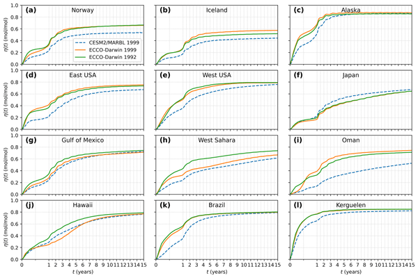
Figure 3 shows a comparison of the OAE equilibration curves (η(t)) for 12 different locations, obtained from one-month pulse additions of alkalinity in January. For the ECCO-Darwin model, two runs were conducted at each location in 1992 and 1999 to obtain a measure of interannual variability. In many locations, substantial differences between the models are observed, typically larger in magnitude than the interannual difference between the two ECCO-Darwin model runs. In general, the ECCO-Darwin model appears to predict faster equilibration than CESM2/MARBL, the only exception being the alkalinity release in the Kuroshio Current (labelled “Japan”). The largest differences are observed on the west coast of the Sahara, off the coast of Oman and for releases in the North Atlantic Ocean. The most extreme difference is observed at the Oman location in the Indian Ocean, where the two models disagree up to 50 % over the majority of the simulation period, with the discrepancy reducing to 25 % by 15 years. Locations near deep-water formation regions, such as offshore of Iceland and Norway, also yield substantially different results, with CESM2/MARBL having 25 % lower uptake compared to ECCO-Darwin.

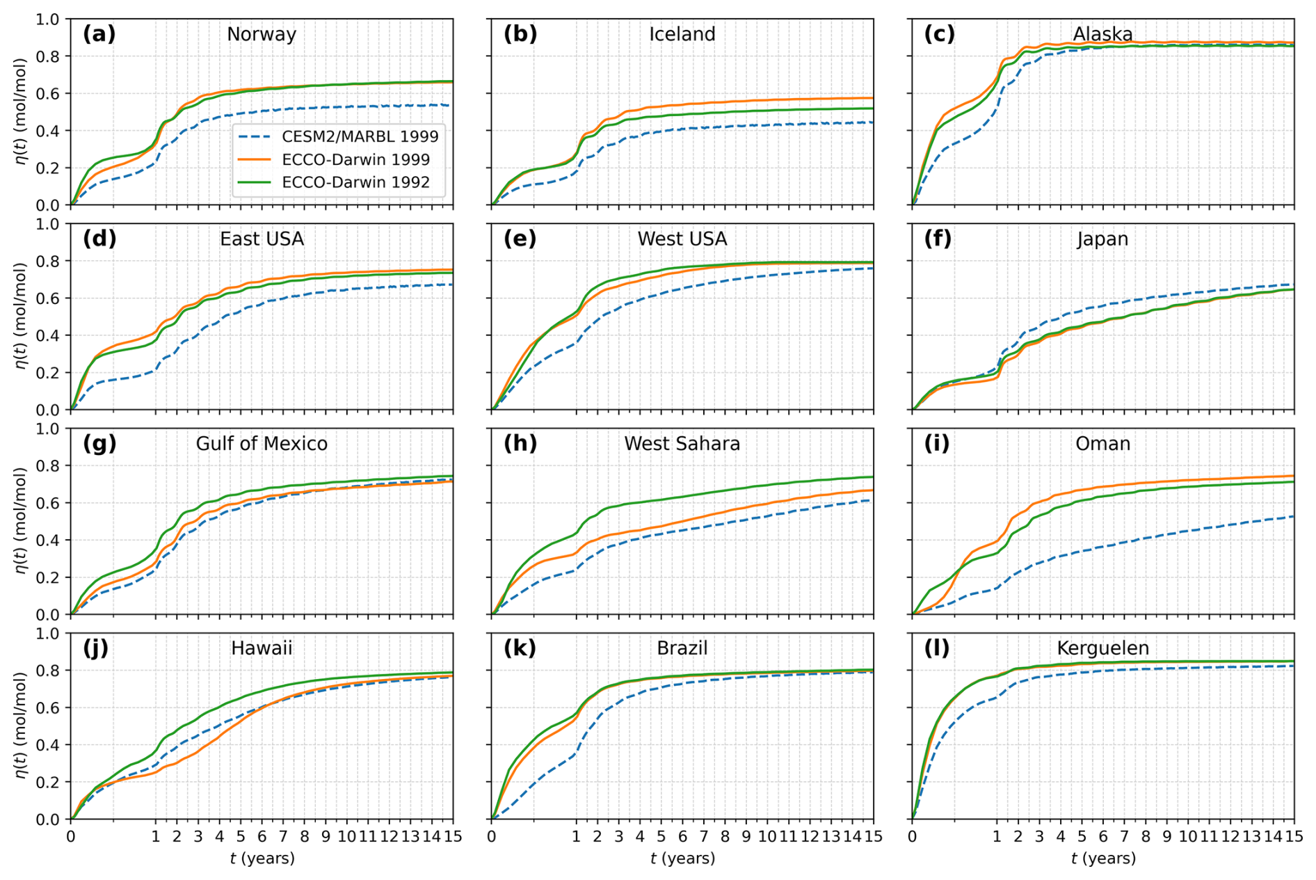
Figure 3 Comparison of OAE uptake efficiency for CESM2/MARBL and ECCO-Darwin at 12 selected locations.

In all locations, uptake differences are most pronounced during the first 7 years after release, where η(t) can vary up to 50 % in extreme cases (such as Oman) but generally differs by ≈10 %–20 %. Subsequently, in some locations, the equilibration curves then begin to converge again, as the equilibration proceeds towards the theoretically maximal value of ≈0.85 – the value of which is determined solely by the carbonate chemistry equilibria (Renforth, 2012). This suggests that the models have relatively good agreement in terms of carbonate chemistry, which is expected. However, this convergence is not observed in the North Atlantic Ocean, where the equilibration differences developed by year 7 do not begin to dissipate. Likewise, the residual differences for the Kerguelen location appear stable even after 15 years. Near deep-water formation areas any differences in the initial rate of equilibration have an outsized effect on the progress of the overall equilibration state because equilibration ceases to make progress once the excess alkalinity has been subducted to depth and is isolated from the mixed layer and atmosphere. In other ocean regions, however, un-equilibrated alkalinity is not subducted deep enough and can be transported back into the mixed layer on a 5–20 year timescale (Zhou et al., 2025), accounting for the continued equilibration and convergence of the equilibration curves, despite the initial divergence. In the cases of Oman and West Sahara, a substantial difference remains in year 15, even though the lagging CESM2/MARBL equilibration is still slowly rising. We note that our simulations were not long enough to determine if there would, eventually, be convergence or not.

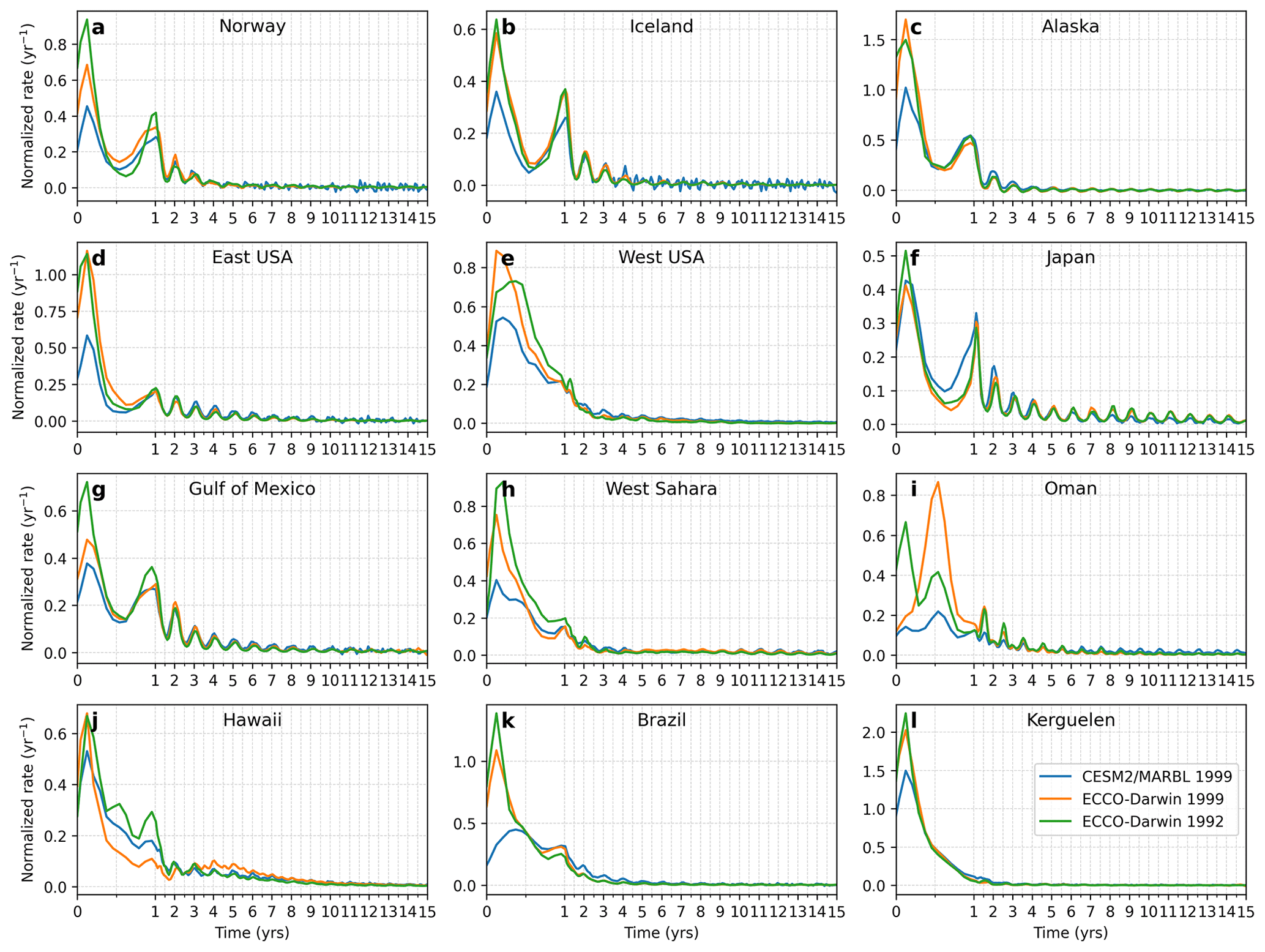
Figure 4 Comparison of the CO₂ uptake rate for CESM2/MARBL and ECCO-Darwin at 12 selected locations (normalized by the total amount of alkalinity added during the pulse).

The divergence between different models results immediately after alkalinity injection. It is therefore instructive to compare the gradient of the η(t) curves, shown in Fig. 4, which compares the normalized rates of equilibration (i.e. $\mathrm{d}\mathit{\eta }\left(t\right)/\mathrm{d}t$) with units yr⁻¹ between the same twelve runs. By far the largest differences between models is observed in the first 6–24 months, after which the rates tend to converge to more similar values. In the most extreme case (Kerguelen), the rates converge by month 4. This means that the majority of the divergence is accumulated in these first months and thus reflects model differences relatively close to the addition site. The strong seasonality of the equilibration rate is also very evident, with peaks occurring in boreal winter for locations located in the northern hemisphere, likely due to winter storms driving vigorous air-sea exchange and deepening of the mixed layer.

We only examined a single location in the southern hemisphere where these peaks would be expected in the boreal summer. However, the location in question, Kerguelen, does not appear to display any seasonal variation in equilibration rate, possibly because equilibration is so fast that it is nearly complete by the second year post injection. The Oman location also displays a strong peaking in equilibration rate in the boreal summer, however this is considerably more pronounced in ECCO-Darwin and appears to be the primary reason for the much faster equilibration in this model. This increased summer equilibration is evident until year 4 or 5 and is much more pronounced in 1999 compared to 1992, accounting for the interannual differences observed.

3.2 Comparison of the interannual variability

As found by a previous study (Yankovsky et al., 2025), interannual variability within an ocean model is generally non-negligible, making comparison between single runs of different models statistically less meaningful. In order to gain insight into the significance of the inter-model differences, we repeated the ECCO-Darwin runs for two different years (1992 and 1999), see Fig. 3.

We found that some locations, such as the Amazon and Kerguelen, exhibited virtually no variability, while subtropical locations such as Hawai'i and the west-Saharan coast have substantial differences. Consistent with prior work (Yankovsky et al., 2025), interannual variability itself varies between locations. In general, the interannual differences were significantly smaller than the inter-model differences. A notable exception was the alkalinity release south of Hawai'i, where the two runs diverged considerably; here the CESM2/MARBL run predicts a CO₂ uptake curve intermediate between the two ECCO-Darwin runs.

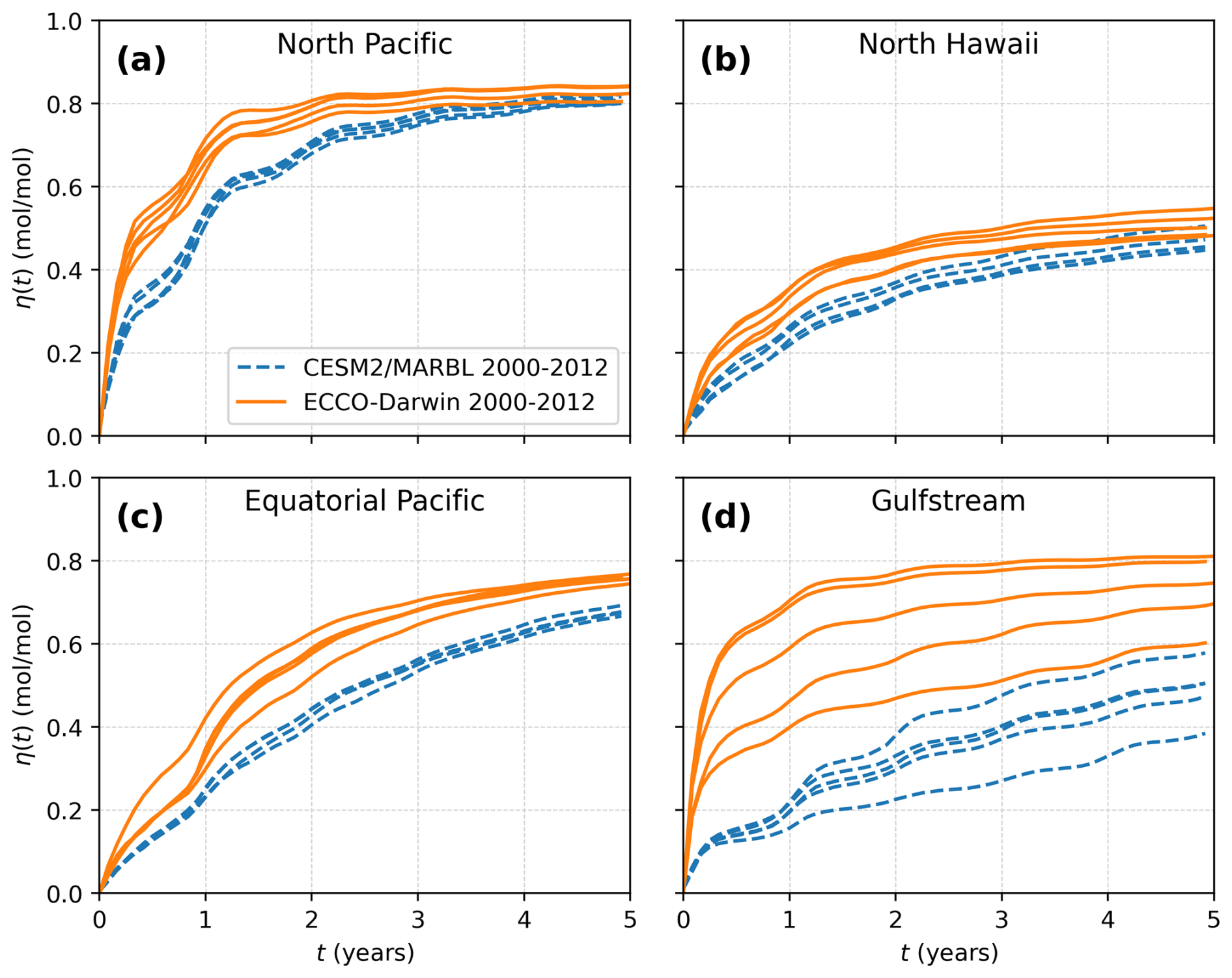
Figure 5 Five-year runs with pulse injections in January of 2000, 2003, 2006, 2009 and 2012, compared with results from Yankovsky et al. (2025) at the same locations and years.

Alkalinity additions in different years are subject to different circulation patterns and gas-exchange conditions, both of which can in principle affect the equilibration curve. Changes in how much alkalinity remains at the ocean surface in the short term, as well as changes in wind speeds, can have a significant effect on the e-folding time of equilibration. Differences in the amount of deep subduction can also affect the apparent η_max if more or less alkalinity is transported to deep waters where it could remain out of contact with the atmosphere for centuries.

To further investigate the interannual variability and compare to the previous study of Yankovsky et al. (2025), we repeated the same runs in four of the same locations and in the same years (2000, 2003, 2006, 2009 and 2012) as in their study, with all injections occurring in January. The alkalinity injections occurred in the same geographical regions (as far as the different grids allowed). The results are shown in Fig. 5.

First, we note that the amount of interannual variability in ECCO-Darwin and in CESM2/MARBL are correlated, with the largest amount observed in the Gulf Stream location, although it is larger in magnitude in ECCO-Darwin compared to CESM2/MARBL for all four cases. Second, it is evident that the model differences are considerably larger than the interannual variability in all four cases, validating the results from Fig. 3. For all four locations, we found that ECCO-Darwin resulted in substantially faster equilibration during the first 5 years compared to CESM2/MARBL, consistent with our results in the other 12 locations presented earlier.

For the injection locations North Pacific, Equatorial Pacific and the Gulf Stream, the interannual variability appears to decrease from year 1–2 to year 5 in both models. For the North Hawai'i location, the interannual variability appears to stay constant in both models. Since our simulations are limited to 5 years here, it is unclear if the interannual variability will eventually converge entirely or not. This likely depends on whether in some years there is deeper subduction than in others, in which case the interannual variability could be persistent over many decades or more.

If, however, the initial variability is due to other factors, one would expect eventual convergence, as has been observed before (Zhou et al., 2025; Yankovsky et al., 2025). An interesting case is the injection north of Hawai'i, which exhibited relatively small interannual variability in ECCO-Darwin as well as CESM2/MARBL. This is in stark contrast to the injection south of Hawai'i (Fig. 3d). It is unclear whether the latter is an outlier or whether the interannual variability is much greater south of Hawai'i.

3.3 Subduction

The equilibration process is dependent on a balance between the rate of CO₂ exchange at the surface ocean and that of subduction processes transporting DIC-deficient water parcels from the surface to depth and hence out of contact with the mixed layer and atmosphere.

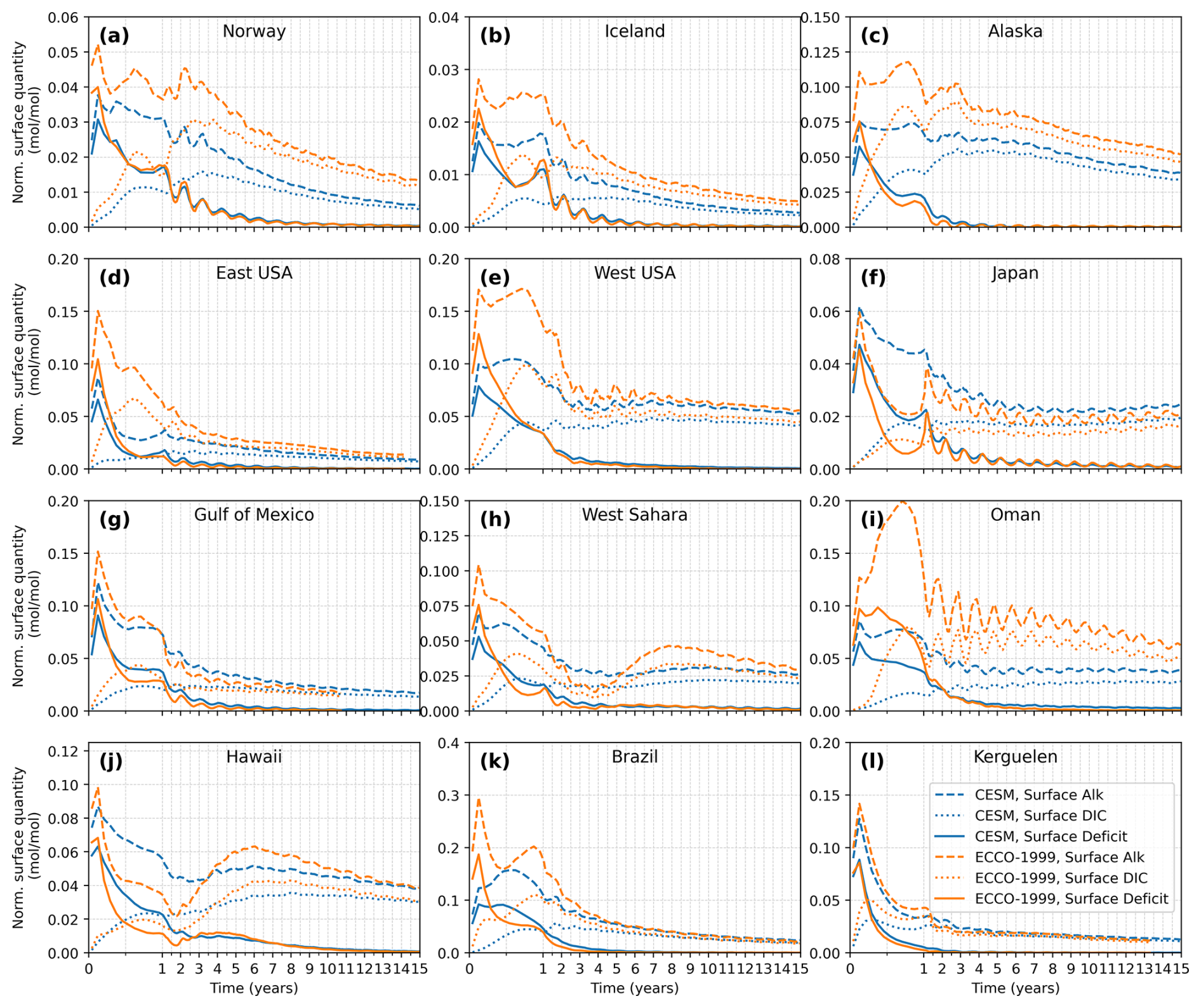
Figure 6 Comparison of the surface excess alkalinity (dashed), excess DIC (dotted) and deficit (solid) for CESM2/MARBL (blue) and ECCO-Darwin 1999 (orange) for the 12 tested locations. All curves are normalized to the total amount of alkalinity added during the injection such that the y-axis is unitless.

Because the excess alkalinity can only contribute to enhanced CO₂ uptake in the surface-ocean layer of the model and because alkalinity is an almost conservative tracer, the fraction of the excess alkalinity retained in the surface ocean is an excellent proxy for monitoring the subduction process of the plume (Zhou et al., 2025). The surface-ocean grid cell in both models is 10 m thick, allowing for direct comparison. Figure 6 shows the surface-ocean fraction of excess alkalinity over time for all 12 locations tested (dashed lines). We find that, in general, a more persistent surface residence of alkalinity also coincides with faster equilibration and vice versa (cf Figs. 3 and 6). Thus differences in the models' predictions of surface alkalinity fraction appear to have a direct effect on the observed equilibration speed. Locations where CESM2/MARBL predicts a smaller surface alkalinity fraction such as Oman, West coast of USA and West Sahara also have slower OAE uptake behavior. For most locations there is a clear qualitative correspondence between a smaller surfaceocean alkalinity fraction and slower equilibration. Likewise, patterns (such as seasonal variations) apparent in one, are visible also in the other.

The most pronounced of these differences in our dataset is found at the Oman location. Here, CESM2/MARBL predicts rapid subduction with equilibration slowing significantly after the first two years but then continuing at a slow pace, due to gradual remixing of the subducted excess alkalinity. In ECCO-Darwin however, a very different kinetics is observed. Here, subduction occurs much more gradually and the equilibration curve does not exhibit a double exponential shape with two characteristic temporal peaks, as was found by Zhou et al. (2025). In the west Sahara location, both models exhibit the steep subduction followed by rebound, but in ECCO-Darwin the rebound is considerably more dramatic and occurs over a different timescale. A more detailed plot of this rebound is shown in Fig. S1 in the Supplement. Overall, equilibration can proceed further at an earlier stage and surface-ocean alkalinity remains higher in ECCO-Darwin compared to CESM2/MARBL.

We note that the surface-ocean alkalinity fraction differs substantially starting from the first data point in the time series, i.e., within one month of alkalinity addition, even though the alkalinity is added only into the surface layer grid cell. Figure 7a shows that surface-ocean fraction of alkalinity during month 1 of the simulations is systematically higher in ECCO-Darwin compared to CESM2, accounting for a significant fraction of the immediate discrepancies in equilibration rate. Since we expect surface-added alkalinity to mix and dilute into the mixed layer around the injection site rapidly, the degree of initial surface-ocean dilution should be directly correlated to the mixed layer depths.

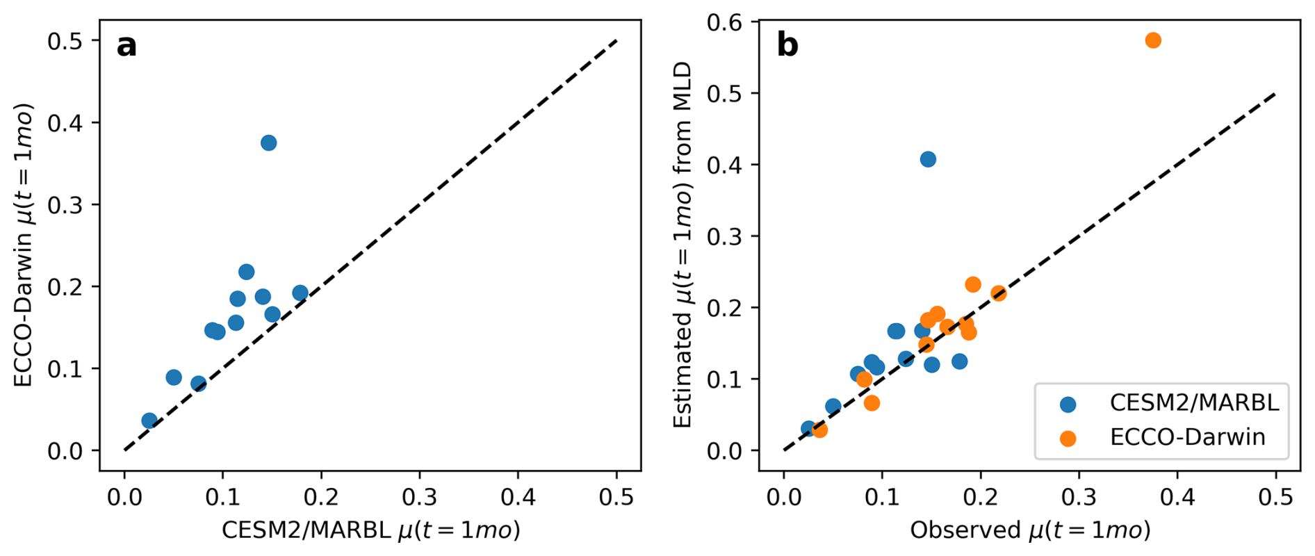
Figure 7 (a) Comparison of surface-ocean alkalinity fraction in month 1 of the simulation (μ) between ECCO-Darwin and CESM2/MARBL. In all locations, ECCO-Darwin retains more alkalinity at the surface ocean compared to CESM2/MARBL. (b) Relationship between the surface-ocean alkalinity fraction in month 1 of the simulation (μ) and the expected surface-ocean alkalinity fraction estimated from the mixed layer depth (de Boyer Montégut et al., 2004) in the injection region. A clear correlation is observed. The three outlier points are all from the location near Brazil, where the mixed layer is extremely thin.

Figure 7b shows that for both models the surface-ocean alkalinity fraction correlates quite well with what would be expected from the estimate of the mixed layer depth (MLD) estimated by the method of de Boyer Montégut et al. (2004) (estimated from the density profile as the shallowest depth where the potential density exceeds its surface value by 0.03 kg m⁻³). For this comparison, we assumed the excess alkalinity would spread evenly throughout the local mixed layer. The excellent agreement demonstrates that mixed layer depth predicted by the models play a central role in determining CO₂ equilibration speeds. In general, it appears that CESM2/MARBL has a considerably deeper mixed layer depth compared to ECCO-Darwin and thus this difference explains a large proportion of the differences in the predicted CO₂ equilibration rate. A direct comparison of the seasonal MLD for both models, for each location, is shown in Fig. S2, together with MLD data from ARGO floats (Holte et al., 2017). In general we observe that the MLDs in ECCO-Darwin agree more closely with the ARGO data than the CESM2/MARBL model.

However, vertical mixing clearly does not explain all the observed differences in equilibration speed. For example, the vertical dilution in the Norway location (Fig. 6a) is quite similar between the models, but the overall equilibration is markedly slower in CESM2. Thus, other factors must contribute more significantly in this location, which will be analyzed further below.

In addition to surface-ocean alkalinity, Fig. 6 also shows the surface DIC (dotted lines) and the surface-ocean deficit (solid lines) as calculated from ΔDIC and ΔAlk (see methods). By definition, in every location where there is initially a higher concentration of surface-ocean excess alkalinity, there is also a greater concentration of deficit and the rate of DIC increase in the surface-ocean layer is proportionally greater. This greater DIC influx, however, begins to quickly reduce the surface-ocean deficit. In many locations, this leads to a convergence of the surface-ocean deficit in the two simulations within the first 6–18 months, even though the difference in excess surface-ocean alkalinity persists. Since it is the deficit that drives CO₂ uptake, this explains the earlier noted convergence of the CO₂ uptake rates. In some cases (Hawaii, Brazil, West Sahara, Alaska), the simulation with the initially higher surface-ocean deficit (ECCO-Darwin) depletes its surface deficit so rapidly that it actually drops below that of the CESM2/MARBL simulation, allowing the latter to catch up in terms of equilibration.

The evolution of the deficit over time is complex, because it is a function both of surface-ocean equilibration (which is determined not only by available surface deficit but also the surface gas-exchange parameters) and subduction below, and remixing of deeper excess alkalinity back into the mixed layer. Such complex dynamics are evident in the Kuroshio current, where, especially in the ECCO-Darwin simulation, the surface-ocean alkalinity and deficit exhibit sharp spikes around March (Fig. 6f). However, in other locations where fresh (unequilibrated) excess alkalinity is brought to the surface over a slower timescale, such as Hawaii (Fig. 6j in years 3–9 and West Sahara (Fig. 6h) in years 6–12 after injection, the deficit does not rise to the same extent, presumably because this signal can equilibrate faster than the influx of fresh, unequilibrated alkalinity.

3.4 Coastal locations

To investigate the effect of near-coast ocean dynamics, which could differ substantially between the two models due to their different horizontal grid resolutions and representation of lateral fluxes, we chose four of the earlier locations and repeated the comparisons in a nearby polygon further out in the ocean. The results are shown in Fig. 8. We found that in all four cases, the agreement between the two models is considerably greater for offshore locations than for near-shore locations. Furthermore, the interannual variation between the ECCO-Darwin runs conducted in year 1999 and 1992 is also reduced in offshore locations compared to their respective near-shore locations. For all four locations, the final values of η(t) at 15 years agreed within ±0.025, but varied as much as ±0.1 for the equivalent near-shore location. These results are consistent with the idea that the coastal 3-D ocean dynamics are complex and difficult to capture correctly in coarse-resolution ocean models, and may differ more between models compared to simulations of open-ocean waters. In particular, one may expect that lower-resolution models might perform more poorly in the near-coast regimes, and that only higher-resolution models can hope to resolve the complex coastal dynamics. Since near-coast dynamics could lead to substantial upwelling or downwelling currents and intense mixing, such differences would be particularly important for OAE equilibration, since only surface-ocean alkalinity can contribute to CO₂ uptake.

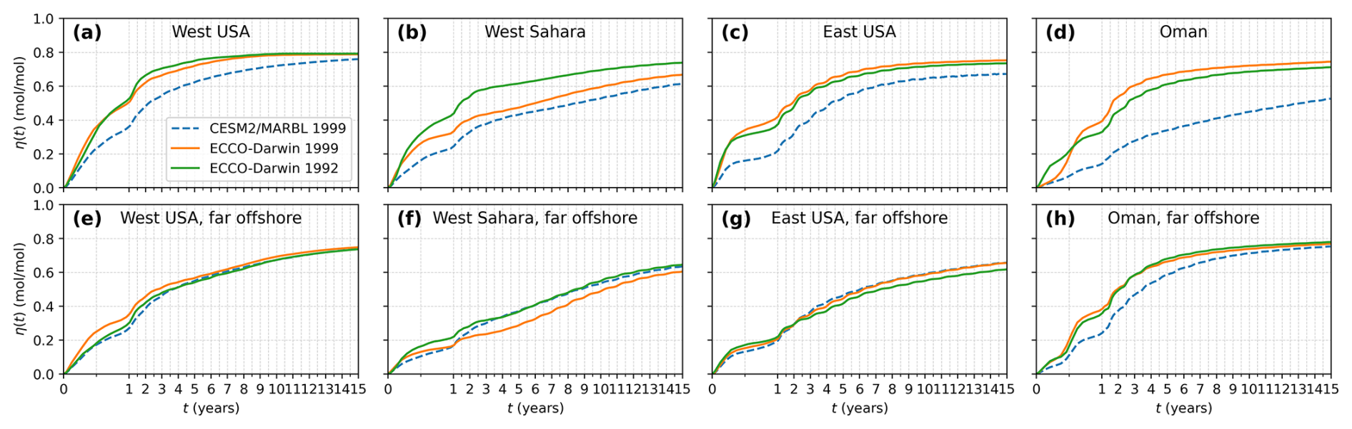
Figure 8 Comparison of OAE equilibration curves from near-coast vs. offshore alkalinity additions.

Figure 9 Comparison of surface-ocean excess alkalinity fraction for the same locations as in Fig. 8.

We strengthen this hypothesis by comparing the surface-ocean alkalinity fraction for the same four location pairs (Fig. 9). In all four cases, the difference in total excess surface-ocean alkalinity proceeds much more similarly in both models compared to each respective near-coast location. This confirms that near-coast subduction and mixed-layer modelling is of primary importance in order to predict the equilibration of near-coast releases. Given that near-coast release of alkalinity is likely to be more economically favorable, this points to a need for greater model certainty in such complex flow regimes. However, the two models we have compared differ in both resolution and parameterization such that we cannot disambiguate which aspect is responsible for the observed differences. Xie et al. (2025) recently reported comparisons between different resolution versions of the same model and found relatively small differences between simulations at 1 and 0.1° resolution; however, locations closer and further from the coast were not explicitly compared.

3.5 Carbonate chemistry

The carbonate chemistry model, in particular at the surface ocean, plays an integral role in the modelling of OAE equilibration. We therefore compare several key quantities between different models, as well as from the data-based OceanSODA product (Gregor and Gruber, 2021) in Fig. 10.

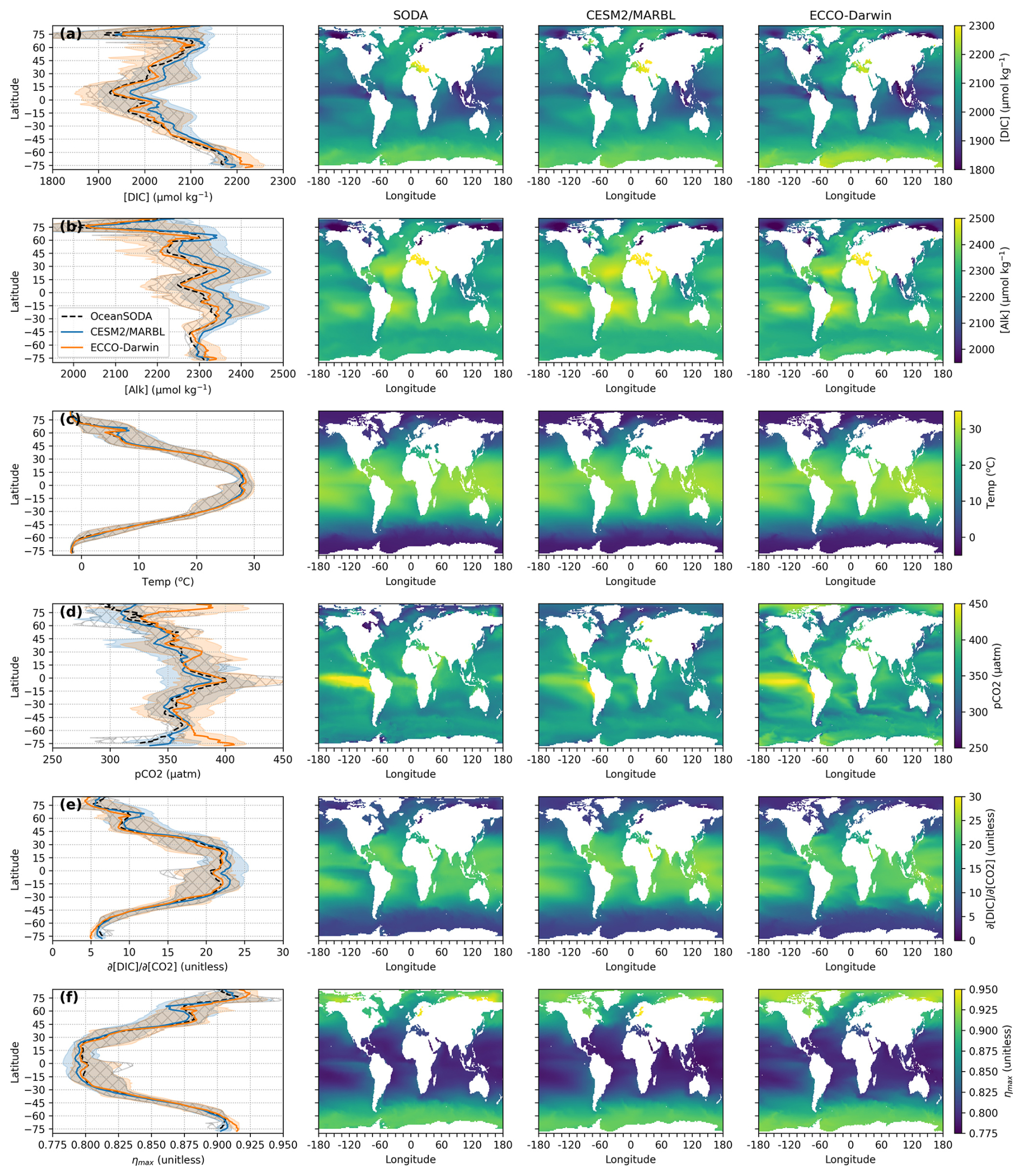
Figure 10 Comparison of surface-ocean carbonate chemistry from CESM2/MARBL model(blue) and ECCO-Darwin (orange), as well as gridded data calculated from OceanSODA (Gregor and Gruber, 2021) (black/hashed) using PyCO2SYS. The pale colored or hashed area denote the 5th and 95th percentiles for each of the three datasets. For the computed meridional averages, the marginal seas were excluded (in particular the Mediterranean, Black, Red, and Baltic Seas, Hudson Bay and the Persian Gulf). Values are time-averaged and plotted against latitude, the spatial axis with the greatest variance. Panels (a) and (b) show [DIC] and total [Alk]. Panel (c) shows temperature. Panels (d)–(f) show derived quantities calculated using PyCO2SYS: (d) pCO₂, (e) the carbonate sensitivity $\mathit{\beta }=\partial \left[\mathrm{DIC}\right]/\partial \left[{\mathrm{CO}}_{\mathrm{2}}\right]$ and (f) ${\mathit{\eta }}_{\max }=\partial \left[\mathrm{DIC}\right]/\partial \left[\mathrm{Alk}\right]$.

Starting with the basic carbonate system tracers [DIC] and [Alk], we find significant differences between the models across latitudes. Compared to OceanSODA, CESM2/MARBL has consistently higher values for both parameters across nearly all latitudes (Fig. 10a, b). ECCO-Darwin exhibits more closely aligned values, although slightly lower than OceanSODA in tropical latitudes. In the Arctic Ocean however, ECCO-Darwin begins to deviate from the observational data, while CESM2/MARBL agrees much more closely. However, because [DIC] and [Alk] have compensatory effects on pH and pCO₂, the differences in pCO₂ are somewhat smaller, with the models showing better agreement with each other and with OceanSODA, and mean discrepancies on the order of 10–20 ppm (Fig. 10d). For comparison, the sea-surface temperature (Fig. 10c) exhibits considerably closer agreement between the two models.

Two important sensitivities are of particular importance for OAE. In the short term, the fact that CO₂ is in comparatively fast equilibrium with bicarbonate ions, vastly increases the capacity of seawater to absorb CO₂, but also increases the e-folding time for air-sea CO₂ equilibration. The term $\partial \left[\mathrm{DIC}\right]/\partial \left[{\mathrm{CO}}_{\mathrm{2}}\right]$ is a key sensitivity which quantifies this effect (Middelburg et al., 2020; Zeebe and Wolf-Gladrow, 2001). It is therefore an important parameter to compare between model implementations. Figure 10e shows its mean values across the latitudes, with larger values leading to slower equilibration. Generally there is quite good agreement, with both models slightly overestimating this sensitivity compared to OceanSODA and therefore overestimating the equilibration e-folding times. The deviation is up to 8 %–10 % for CESM2/MARBL and 2 %–4 % for ECCO-Darwin, with commensurate deviations expected for the equilibration rate constant.

In the long term, after extensive mixing, the equilibration curves will approach a value given by the sensitivity of the carbonate system [DIC] to increases in alkalinity, typically written as $\partial \left[\mathrm{DIC}\right]/\partial \left[\mathrm{Alk}\right]$, since it determines the amount of DIC deficit created per unit alkalinity added. The long-term effect on radiative cooling effected by OAE, given the typical lifetime of CO₂ in the atmosphere, occurs on timescales of hundreds of years, by which point alkalinity releases from most locations (other than those near deep-water formation areas) will be thoroughly equilibrated. Thus, the end point of the equilibration, i.e., the value of $\partial \left[\mathrm{DIC}\right]/\partial \left[\mathrm{Alk}\right]$ is of long-term importance (Zhou et al., 2025; Renforth, 2012) and it is interesting to compare this factor between models. Figure 10f shows that both models agree quite closely, with deviations on the order of a few percent. This suggests that the long-term CO₂ predictions from both models are likely in very good agreement, even if the short-term equilibration e-folding times may differ in each model. This is consistent with a general understanding that the ocean carbonate chemistry is well understood and therefore not a major contributor to the inter-model-variance of OAE efficiency. It is also consistent with our observation that the η(t) curves appear to converge in many locations towards the end of the 15-year period simulated here.

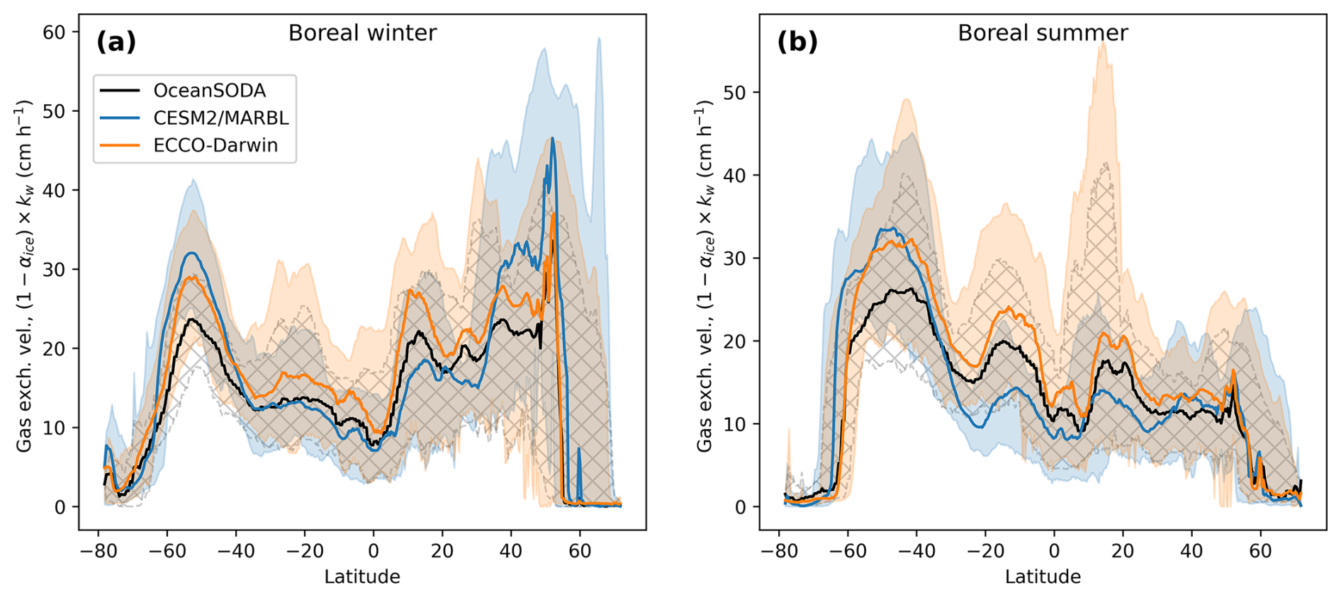
Figure 11 Comparison of the gas exchange velocity k during boreal winter (a) and summer (b) for the year 1999 in CESM2/MARBL, ECCO-Darwin and OceanSODA.

3.6 Wind speed

Wind speed plays a central role in determining the rate of gas exchange (Meyer et al., 2018) across the ocean-atmosphere boundary, as the gas transfer velocity k is typically parameterized as a function of the square of the wind speed (Wanninkhof, 2014). Greater wind stress can also increase vertical mixing in the upper ocean, contributing to changes in the surface-ocean fraction of alkalinity.

Figure 11 compares the k parameters calculated for the two models being compared here and for OceanSODA. The contribution of sea ice has been included in this comparison. The values for k agree in general, but the details differ substantially. In the boreal summer for example, in the subtropical zones around ±18°, ECCO-Darwin has k parameters that are nearly 40 % higher than those observed in CESM2/MARBL.

This can be partially explained by the different gas exchange parameterizations in the two models, as noted by Xie et al. (2025). ECCO-Darwin uses the older, but widely- adopted parameterization from Wanninkhof (1992) with a higher coefficient of 0.337, while CESM2/MARBL uses a more recent estimate from Wanninkhof (2014) with a coefficient of 0.251, which is roughly 25 % lower. However, the observed differences in k differ in a more complex way than a simple scaling; the k values in ECCO-Darwin are higher than those from CESM2/MARBL in equatorial regions but lower in polar regions, therefore affecting alkalinity releases at different latitudes in different ways (as will be shown later).

3.7 Biological processes

As described in the methods, we examined the importance of simulating the soft tissue pump and other biological processes on the equilibration curve by comparing the results of the regular ECCO-Darwin model with an ablated version in which computation of these systems was disabled. The results are shown in Fig. 12.

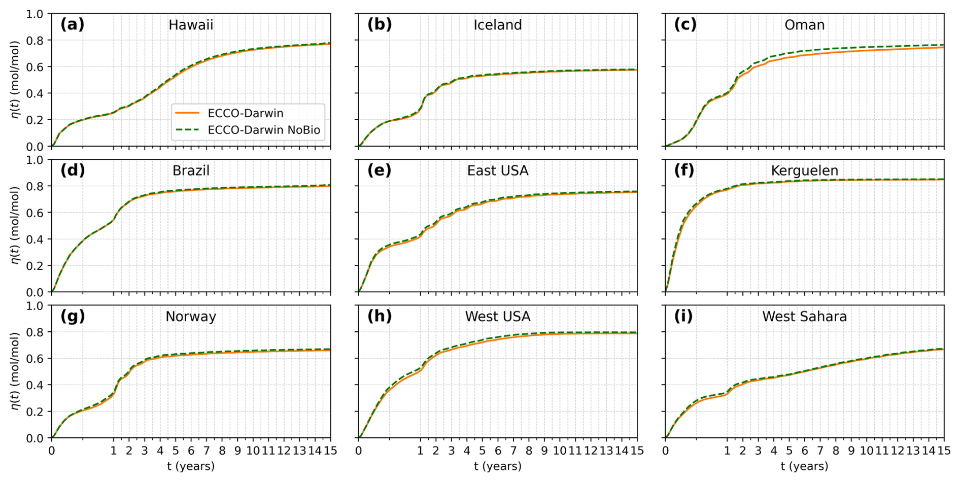
Figure 12 Ablation of biological modelling. The runs labelled “ECCO-Darwin NoBio” have been conducted without biological processes – only the gas-exchange component of the model was enabled. The η(t) were also calculated against a separate reference simulation, likewise without biological processes.

Despite the rather abrupt perturbation to the model (Fig. S3), the results show virtually no difference in the equilibration curves with or without biological processes enabled. Despite the sudden removal of biological activity, which causes a steady change in surface-ocean DIC and Alk, these changes are virtually equal in the perturbed and the reference simulations and thus for the purpose of calculating the ΔDIC induced by the alkalinity pulse, they appear to cancel. This suggests that OAE impulse response functions can be simulated relatively accurately without reliance on detailed biological models, provided the background carbonate state (vertical DIC and Alk gradients) is accurate to start with. A small difference was observed at the Oman location, however its root cause could not be determined at this time.

We note that the quantities of alkalinity added in these simulations are quite small and ocean variables such as pH and carbonate saturation are not dramatically changed. Thus, the rate of biological processes is not impacted significantly. For real-world deployments of OAE, this situation may be quite different and these results here do not apply to the question whether large-scale deployments of OAE could affect biological processes, or cause secondary positive or negative CO₂ uptake feedbacks.

It should be noted that 29 out of 31 tracers were turned off for this experiment, which reduces the computational load substantially. Given the small impact of biology relative to the large impact of circulation, and in particular vertical processes and subduction, it is likely beneficial to focus computational expenditure on higher-resolution models rather than sophistication of biological modelling for the purpose of calculating accurate OAE impulse response functions. We note that for each deployment time a no-biology reference simulation must also be branched off the main simulation. However, if many OAE perturbations are being tested at different locations (as in Zhou et al., 2025), the computational cost savings can be substantial overall.

3.8 Interaction of plume trajectory and surface exchange parameters

Thus far, the analysis has focused on the various aspects of the ocean models which conceivably contribute to CO₂ equilibration dynamics, one at a time: overall surface-ocean dilution and parameterization of gas transfer (i.e., wind speeds, carbonate chemistry parameters and biological processes). However, for any particular release location, the relative importance of these parameters is dependent on the particular model trajectory the DIC deficient plume takes, for example, which gas transfer velocities will be encountered by the space-time evolving plume. To disentangle these effects, at least to the extent feasible, we devised a more specific approach which examines changes to the equilibration rate based on changing one component of the plume at a time as described in detail in the methods section.

There are two different approaches this analysis takes. First, we investigate the effect of changing parameters sets or individual parameters, given a fixed plume trajectory. This probes the parameterization of the gas exchange, separate from the question of how each model predicts the trajectory of any given plume. As described in the methods, each parameter can be considered in isolation. Second, we investigate the effect of different horizontal plume trajectories intersecting a constant set of gas exchange parameters (gas-exchange velocity k and carbonate sensitivity β). This probes the importance of the predicted flow pattern of each model, separate from the parameterization itself.

Figure 2 illustrates an example of alkalinity release near Alaska where three different plume trajectories are overlaid over the gas exchange parameter k. One can clearly see how equilibration will speed up if the plume intersects high-wind regions in the North Pacific and avoids the sea-ice covered regions north of Bering Strait. Likewise, changes in the k parameter would only influence the equilibration if the changes occur along the actual DIC-deficient plume trajectory.

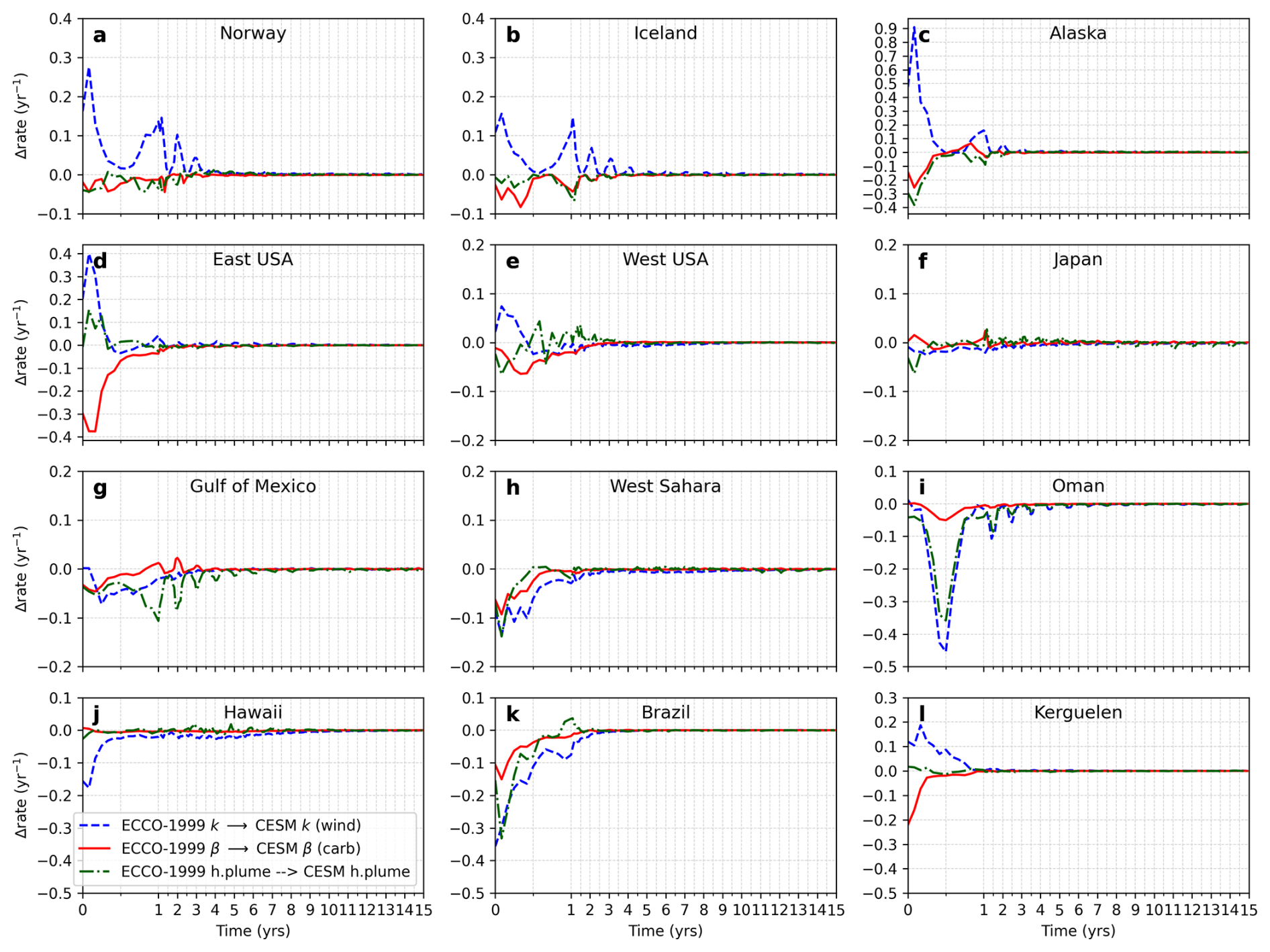
Figure 13 Change in the normalized equilibration rate in the 1999 ECCO-Darwin run when changing only one term at a time to the equivalent one from CESM2/MARBL 1999. Positive values indicate faster parameterization in CESM2/MARBL, negative values indicate faster equilibration in ECCO-Darwin. Change due to wind parameterization (k) is shown in the dashed blue line. Change due to carbonate system parameterization is shown in the solid red line. Change due to different horizontal plume realizations is shown in the dash-dot green line.

Figure 13 shows the changes in the equilibration rate with respect to the exchange of changing different components of the rate constant expression (Eq. 14). In most locations, the wind parameterizations appear to play a large role in determining equilibration rates. Interestingly, in polar locations the equilibration appears to be consistently slower in ECCO-Darwin (e.g. Norway, Iceland, Alaska and Kerguelen), while for tropical and subtropical locations it appears to be somewhat faster (e.g., Gulf of Mexico, Oman and Brazil). This is consistent with the general observation that k_w values from ECCO-Darwin exceed those from CESM2/MARBL in the tropics, but are generally lower compared to those from CESM2/MARBL towards the poles (see Fig. 11). This pattern is especially pronounced in the boreal winter. The most extreme difference is found in the Alaska release location, where considerably slower winds are encountered in the ECCO-Darwin 1999 run compared to CESM2/MARBL, especially during the first 6 months of the simulation.

The influence of the sea-ice parameterization was not separated in this plot, since its influence is very small compared to the other parameters (<0.01 yr⁻¹), however it is singled out in Fig. S6 for the interested reader. As expected, sea-ice cover only influence the three most northern injection locations, Norway, Iceland and Alaska (Fig. S6a, b and c). The influence only appears after 1 year, once part of the plume has had a chance to reach sea-ice covered areas. As expected, for more equatorial release locations, sea-ice coverage has no influence (Fig. S6e–l), except for the Gulf Stream location (East USA) (Fig. S6d), where some differences are evident after year three when the alkalinity reaches the North Atlantic Ocean and encounters the presence of sea ice.

Figure 13 also shows the influence of the carbonate system (β, in red), which is much more modest compared to wind effects. In general, the carbonate parameters in ECCO-Darwin favor a slightly faster equilibration compared to CESM2/MARBL. This is consistent with earlier observations that the carbonate system description is very similar in the different models. These results are consistent with the earlier comparison of β across latitudes (see Fig. 10 e), where β in ECCO-Darwin is consistently smaller than in CESM2/MARBL, resulting in faster equilibration. Once the plumes have spread widely, its contribution becomes practically negligible; however, early, when the plume is more localized, the difference can be significant in some locations (e.g., East USA, Brazil and Kerguelen). In particular, on the east coast of North America the carbonate parameterization of ECCO-Darwin predicts a considerably faster equilibration compared to CESM2/MARBL in the first 3 months after injection (Fig. 13d); however, the effect is somewhat counteracted by a slower wind parameterization during the same time period.

Finally, Fig. 13 also shows the relative change in the CO₂ equilibration rate, when the horizontal distribution of the surface-ocean deficit is changed from ECCO-Darwin to CESM2/MARBL, while keeping the parameters and the total amount of surface-ocean deficit constant. Since the horizontal transport and time evolution of the plume reflect physical bulk flow predicted by each model, these curves represent the extent in which these flow predictions can cause changes in the CO₂ equilibration. We note that these changes are relatively modest in most cases, similar in magnitude as model differences in carbonate system parameterization. However, in the locations Oman and Brazil, they appear to be on par with changes in wind parameterization. Especially in Oman, the horizontal plume trajectory appears to be a major contributor to the peak equilibration events that occur during boreal summer (i.e., in months 6, 18, 30 etc).

4 Limitations and Conclusions

Due to the complexity of the variables at play, the sheer number of different ocean models that have been developed and the lack of direct measurements of CO₂ equilibration at basin scale, this work cannot possibly give a comprehensive conclusion to the question of how accurate ocean models are at predicting OAE-based CO₂ uptake. This paper is therefore intended as a first preliminary exploration of the possible effects of different model parameterizations and hopes to serve as a starting point for further research; many aspects and interesting questions have not yet been explored due to limitations in available computing and analysis resources. Only two models have been compared, thus it is difficult to know if the magnitude of model differences observed here are representative of the variance across a larger group of models or if one of the two models examined here is an outlier. Moving forward, a more-comprehensive model inter-comparison is needed to answer this question. All alkalinity releases were conducted in January, so further work remains to quantify how these discovered differences translate to other release months at various global locations. This is important, since previous work has revealed considerable seasonal differences in uptake curves (Zhou et al., 2025; Suselj et al., 2025), plume trajectories and background air-sea equilibration timescales (Jones et al., 2014). Interannual variance was also only addressed minimally for most locations, with only a small amount of insight gained for a selected few locations. A major limitation to our conclusions is of course the fact that we were only able to compare two models; thus a large-scale OAE inter-model comparison is sorely needed to gain more insights into the model variance. Overall, however, much more observational data will be required to make progress on model accuracy.

While the two models used here have somewhat different resolution (1° vs $\mathrm{1}/\mathrm{3}$°), we are unable to disambiguate whether the differences in plume trajectories arise from differences in forcing parameterization or the resolution itself. However, resolution differences within the same model framework were recently studied by Xie et al. (2025) and relatively small differences were found, suggesting that the strong differences observed in the present study arise from differences in the forcing and parameterization, rather than the explicit grid resolution. However, there is the caveat that resolution hierarchies in other models may exhibit more profound differences owing to grid resolution, depending on scale-dependent parameterization choices employed as resolution changes. Further, Xie et al. (2025) only investigated resolution differences down to 0.1°, which may not be fine enough to reveal sufficient effect of complex coastal-ocean flows. Coastal areas are regions of intense submesoscale dynamics and interactions with bathymetry, known to create higher vertical velocities, thus more research will be necessary to establish the importance of submesoscale-resolving simulation on OAE efficiency calculations.

We have compared OAE-based CO₂ uptake curves for two different resolution models, the 1.0° CESM2/MARBL-based model used by Zhou et al. (2025) and the ECCO-Darwin $\mathrm{1}/\mathrm{3}$° model, based on 12 pulse-release experiments conducted in both models in the month of January at matched locations. The ECCO-Darwin-based experiment was also repeated in year 1992 and 1999. We find that significant and complex differences in the equilibration trajectories are evident in almost all locations. In general, ECCO-Darwin predicts faster equilibration timescales compared to CESM2/MARBL. The most significant deviations occur in the near-term (years 1–7), with a degree of convergence towards $\mathrm{\Delta }\mathrm{\Sigma }\mathrm{DIC}/\mathrm{\Delta }\mathrm{\Sigma }\mathrm{Alk}\approx \mathrm{0.85}$ observed in many but not all locations. Near-coast locations were also found to have greater disagreements than offshore locations.

We further examined the root causes of these differences, including primary differences in the gas-exchange parameterization itself (wind speeds, sea-ice cover and carbonate parameters) and secondary differences in the flow field predicted by the various models. Overall, the largest contributor was found to be the mixed layer depth, vertical transport and deeper mixing of surface alkalinity, consistent with results from Suselj et al. (2025). The second-largest contributor was the gas exchange (wind) parameterization. More minor changes arise from differences in the carbonate system parameters, which were found to be generally aligned between models. Horizontal plume trajectories also were found to play a role, however this varied considerably from location to location. While our analysis tries to separate the effect of gas-exchange parameters from that of the bulk flow, the two are of course not cleanly separable, since the gas exchange history affects the spatial distribution of the remaining deficit. The role of biological activity was also assessed, and its effect on the shape of the equilibration curves was found to be almost negligible, at least during the pulse trajectory. However, the biological model is critical to setting up the correct ocean biogeochemistry initial conditions, in particular the vertical Alk and DIC gradients.

Given the variations observed, even when only examining two models, much more experimental data will be needed to constrain simulations and narrow the variance observed in OAE uptake predictions. In particular, it appears that vertical transport is not sufficiently constrained, especially in near-coastal areas, where the dynamics and three-dimensional flows may be quite complex. Higher-resolution models or coarser models with unstructured fine-scale grids in the coastal zone (Ward et al., 2020) should in principle yield more-realistic flow patterns and estimates of vertical mixing towards the coast. Thus, it would be useful for future work to examine whether high-resolution models give closer mutual agreement compared to coarser-resolution models, especially across the coastal and nearshore zone (Anderson et al., 2025). It may be, however, that more high-resolution experimental data, especially for deeper parts of the ocean, will be needed to verify and constrain simulations. Besides differences in model resolution and parameterization, we note that the inter-model differences described in this paper may also arise from the use of physical and biogeochemical data assimilation in ECCO-Darwin, which could lead to more-accurate representation of the physical-biogeochemical ocean state. Notably, CESM2/MARBL is known to exhibit several biases in ocean physics, in particular mixed layer depth, which will impact OAE equilibration timescales (Griffies et al., 2009; Danabasoglu et al., 2014). The inherent limitations of using ocean-only models, vs. fully-coupled Earth System Models (ESMs) have also not been explored sufficiently yet, where reservoir feedbacks (Oschlies, 2009) or long-term changes to calcification rates at large deployment scales (Bach et al., 2019; Bach, 2024) could potentially play a role. However many of these effects occur on longer timescales and may not directly influence the equilibration speed of individual OAE deployments.

On the other hand, since the behavior of small water parcels close to the original injection site is inherently chaotic, there may exist inherent limits to the reliability any simulation can achieve even in the limit of realistically modelled physics, when the precise motion and forcings at the time of release can never be measured to a sufficiently fine degree. Here, only direct experimental tracking of the spreading plume can help fill the knowledge gap. Once sufficiently dispersed, effects of local chaos are reduced and a more-averaged, and more-aggregate behavior could be expected, amenable to ocean models. In that sense, the ultimate MRV approach will likely require a close interplay between experimental near-field measurements and far-field simulations.