Redox-network reconfiguration inferred from the ln[O₂]–E_h relationship under mixed-potential conditions in a shallow pond time series

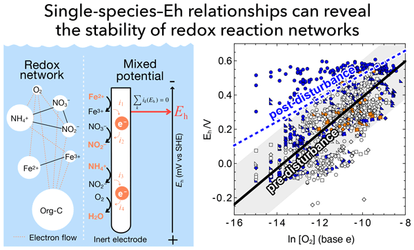
Oxidation–reduction potential (E_h) is widely used as an in situ indicator of redox conditions in aquatic environments, and field electrodes typically record a mixed potential generated by multiple concurrent interfacial redox reactions. Beyond a simple Nernstian interpretation based on a single redox couple, here we ask what mechanistic information can be extracted from an observed relationship between E_h and a single chemical species under mixed-potential conditions, focusing on dissolved oxygen. Using a linearized mixed-potential formulation, we show that the sensitivity $\partial E_{\mathrm{h}}/\partial \ln a_x$ can be decomposed into (i) Nernstian contributions and (ii) kinetic contributions from multiple reactions. Consequently, an approximately constant log-linear ln [O₂]–E_h sensitivity does not require dominance by a single couple (e.g., O₂ $/$ H₂O); it can also arise when the effective reaction set contributing to the mixed potential and their relative weights remain approximately invariant, suggesting that this relationship can serve as a compact indicator of redox-network stability.

To examine whether such slope stability and breakdown are observable in the field, we apply this interpretation to a 21-month, multi-site time series from a constructed shallow pond in Japan, where dissolved oxygen and electrode redox potential were co-measured at weekly fixed depths and along biweekly vertical profiles. Channel excavation produced a pond-wide electrical conductivity anomaly, and change-point detection was used to define pre- and post-disturbance regimes. During the pre-disturbance regime, the ln [O₂]–E_h slope was relatively stable across sites. After disturbance, the inflow-proximal site exhibited a weakened slope and systematically elevated E_h relative to the pre-disturbance baseline; notably, baseline-referenced E_h deviations peaked after the EC anomaly had largely relaxed, and a follow-up survey in February 2025 indicated partial recovery. Co-located E_h and oxygen measurements can thus provide a simple, screening-level indicator of departures from a site-specific redox baseline that are consistent with disturbance-driven changes in effective redox conditions and recovery, while recognizing that complementary speciation measurements remain necessary to identify the underlying redox processes and dominant redox couples.

1 Introduction

Redox processes regulate the transformations of carbon, nitrogen, sulfur, iron, and other redox-sensitive elements, thereby shaping nutrient cycling, organic-matter degradation, and the mobility and reactivity of heavy metals in aquatic environments (Borch et al., 2010; Violante et al., 2010; Schlesinger and Bernhardt, 2013; Tandon and Singh, 2016; Lau et al., 2018; Linnik et al., 2023). Oxidation–reduction potential (E_h) is therefore widely used as a convenient in situ indicator of “oxidizing” or “reducing” conditions in natural waters (Whitfield, 1969; Stumm and Morgan, 1996; Luther, 2016).

In natural waters, multiple redox couples coexist and exchange electrons at different rates under the combined influence of transport, chemical reactions, and microbial metabolism (Stefánsson et al., 2005; Grundl, 1994; Grenthe et al., 1992). These coupled processes constitute a redox reaction network that establishes concentration gradients of oxidants and reductants in the bulk solution and determines their local activities at the electrode surface (Fig. 1). As a result, field E_h measurements generally reflect a mixed potential, E_mix, at which the net interfacial current vanishes,

$$\begin{array}{}\text{(1)}& \sum _k{i}_k\left(E_{\mathrm{mix}}\right)=\mathrm{0}.\end{array}$$

Here i_k(E) denotes the partial current associated with reaction k at electrode potential E. Consequently, E_h cannot, in general, be interpreted as a quantitative proxy for any specific redox couple (e.g., Fe(III) $/$ Fe(II), Mn(IV) $/$ Mn(II), NO${}_{\mathrm{3}}^{-}$ $/$ NO${}_{\mathrm{2}}^{-}$, SO${}_{\mathrm{4}}^{\mathrm{2}-}$ $/$ HS⁻), nor for individual reaction fluxes. Consistent with this mixed-potential view, prior studies have shown that measured E_h does not necessarily track the Nernst (equilibrium) potentials of selected redox couples in natural waters (Whitfield, 1974; Lindberg and Runnells, 1984; Teasdale et al., 1998; Ramesh Kumar and Riyazuddin, 2012; Bowman et al., 2025).

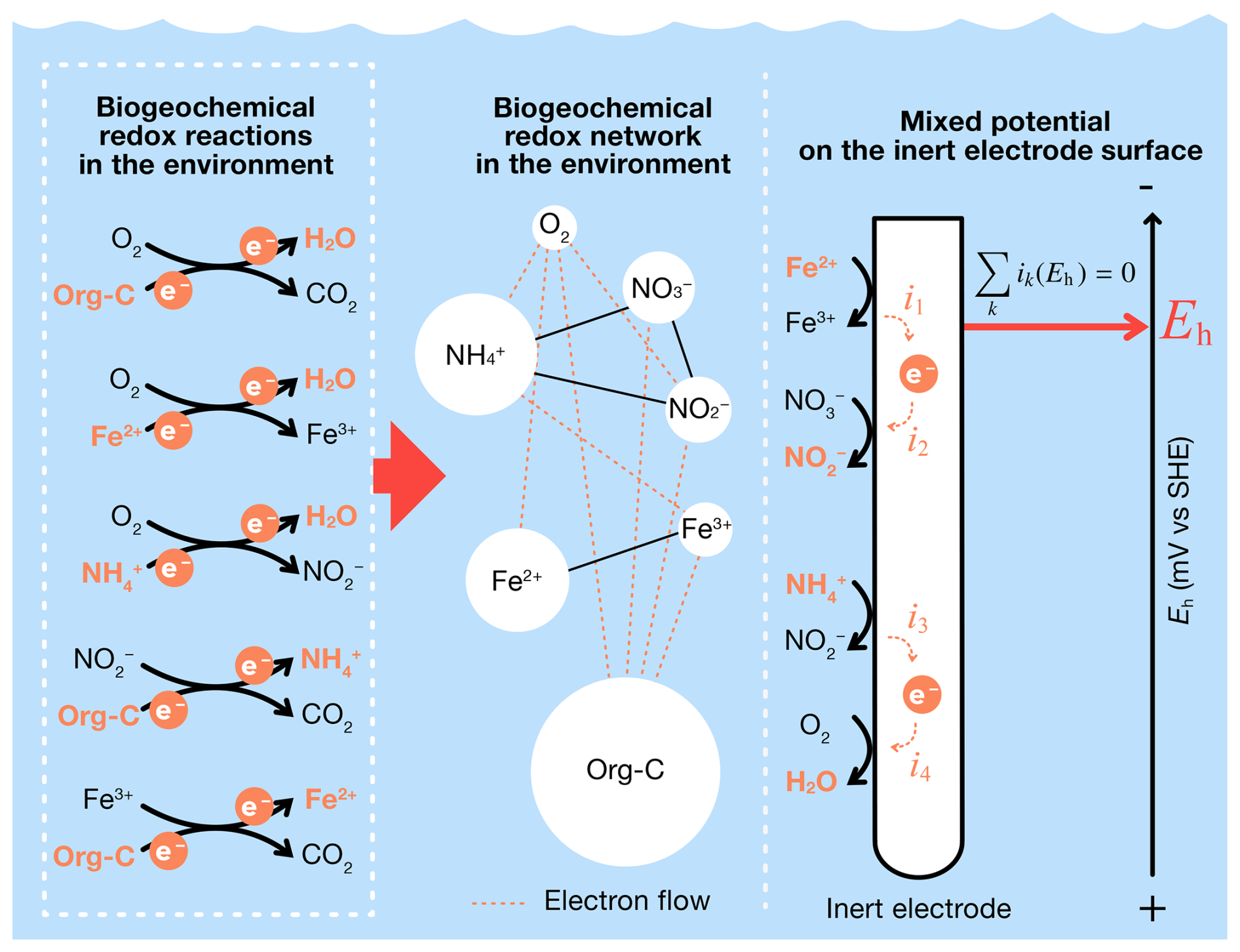
Figure 1 Conceptual schematic illustrating how E_h measured by an inert electrode emerges as a mixed potential from a biogeochemical redox reaction network. Left: Representative biogeochemical redox reactions in natural environments, in which multiple oxidants and reductants exchange electrons through microbial metabolism, chemical reactions, and transport processes. Middle: These reactions collectively form a redox reaction network that establishes electron flows and concentration gradients of redox-active species (e.g., O₂, ${\mathrm{NO}}_{\mathrm{3}}^{-}$, ${\mathrm{NO}}_{\mathrm{2}}^{-}$, ${\mathrm{Fe}}^{\mathrm{2}+}/{\mathrm{Fe}}^{\mathrm{3}+}$, ${\mathrm{NH}}_{\mathrm{4}}^{+}$, and organic carbon) in the bulk environment. Right: At the inert electrode surface, each redox couple contributes a partial current i_k(E), and the measured potential E_h adjusts to a value at which the net interfacial current vanishes, ${\sum }_k{i}_k\left(E_{\mathrm{h}}\right)=\mathrm{0}$.

Although mixed-potential theory does not, in general, ensure a one-to-one mapping between E_h and any single chemical species, in practice E_h often covaries with the activity of particular oxidants, reductants, or redox couples, and empirical relationships have been reported across diverse field settings (e.g., Seto and Akagi, 2005; Włodarczyk et al., 2007; Auqué et al., 2008; Winkel et al., 2008; Ioka et al., 2011; Jahangir et al., 2012; Zhai et al., 2012; McAleer et al., 2017; Silva et al., 2017; Aladejana et al., 2020; Cuoco et al., 2022). This raises a key question: under what mechanistic constraints can a seemingly simple E_h–species relationship arise from mixed-potential dynamics?

Here we revisit E_h explicitly as a mixed potential and ask what information can, and cannot, be extracted from its relationship with the activity of a single species. Rather than treating E_h as a proxy for a specific redox couple, we interpret it as a reduced-order observable emerging from a high-dimensional reaction network. Within this framework, we show that the sensitivity of E_h to ln [O₂] provides a compact indicator of the effective stability of the reaction set contributing to the mixed potential. Applying this approach to a 21-month time series from a constructed pond, we quantify site-dependent differences in redox-network stability and identify a disturbance-induced shift in ln [O₂]–E_h sensitivity followed by gradual recovery.

2 Materials and Methods

2.1 Monitoring site

A small artificial pond (≈ 10 m³; 34°41^′14.5^′′ N, 135°49^′45.9^′′ E) in Nara Prefecture, Japan, served as the study site (Fig. 2). The pond is surrounded by trees and receives substantial inputs of leaf litter in autumn. The bottom substrate consists primarily of gravel mixed with decomposed leaves, and no aquatic macrophytes are present. Leaf litter was not actively removed during the monitoring period and was left to decompose within and around the pond. Water depth varies spatially, exceeding 40 cm at Site A1 and A0, ranging from 20 to 40 cm at Site B, and remaining below 20 cm at Site C.

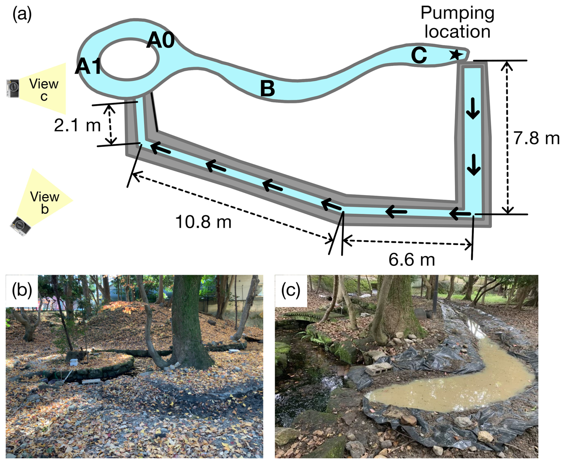
Figure 2 Overview of the constructed pond and sampling locations. (a) Schematic plan view showing the positions of monitoring sites A1, A0, B, and C, together with the open peripheral side channel and pumping location. Arrows indicate the direction of water flow driven by intermittent pumping, distances between segments are provided for scale, and viewpoint markers indicate the approximate viewing directions of photographs shown in panels (b) and (c). (b) Photograph of the pond environment illustrating the forested setting and substantial leaf-litter accumulation around the pond. (c) Photograph taken on 15 June 2023 after construction of the peripheral channel, showing sediment-laden inflow that represents the major physical disturbance analyzed in this study.

The pond is enclosed on three sides by a waterproof mortar structure that prevents lateral inflow or outflow. To promote water circulation, the open peripheral side channel shown in Fig. 2a was constructed in two stages: an initial manual excavation in August 2022, followed by a larger-scale mechanical excavation in May–June 2023. After channel construction, water was pumped intermittently (daytime only) using a solar-powered system. Pumping volumes measured during 26 August–14 September 2022 averaged 499 L d⁻¹ (range: 124–1300 L d⁻¹). The short-term on/off frequency of the pump was not continuously logged. Following the June 2023 excavation, sediment-laden inflow from freshly disturbed soils was observed to enter the pond (Fig. 2c).

2.2 Weekly stationary and biweekly vertical profile monitoring

From July 2022 to March 2024, water-quality monitoring was conducted weekly at four sites (A0, A1, B, and C) using portable instruments. Site A1 was monitored throughout the study period (7 July 2022 to 30 March 2024) as the primary reference site, whereas Sites A0, B, and C were monitored during partially overlapping intervals due to logistical constraints. A follow-up vertical-profile survey was additionally conducted in February 2025 using the same instrument and protocols.

At each site, measurements were taken at two depths (5 cm below the water surface and near the bottom) on a weekly basis. In addition, vertical profiles were obtained at 5 cm intervals from the water surface downward every two weeks. All measurements were performed between 10:00 and 15:00 (local time).

Measured parameters were pH, dissolved oxygen (DO), oxidation–reduction potential (ORP, reported as E_h), electrical conductivity (EC), water temperature, and water depth. pH was measured using a PRN-41 (Fujiwara Scientific Co., Ltd., Japan), and water depth was measured using a measuring stick. DO, ORP, EC, and water temperature were measured using a LAQUA-WQ310 (Horiba Scientific, Japan). The DO optode was model 300-D-2, the ORP electrode was model 9300-10D (reference electrode: 3.33 mol L⁻¹ KCl Ag $/$ AgCl; indicator electrode: Pt), and the EC electrode was model 300-C-2 (sensor head) equipped with a 300-4C-C cartridge. Manufacturer specifications (measurement range, resolution, and stated accuracy/repeatability) for all sensors are summarized in Table A1. The pH and DO sensors were calibrated before each field survey following the manufacturer’s protocols. The ORP and EC sensors were checked against standard solutions prior to the start of the monitoring period, but were not routinely recalibrated thereafter. Before each survey, electrodes were rinsed with distilled water, gently agitated, and visually inspected for deposits. The same instrument and electrodes were used throughout the monitoring period. All measurements were performed in situ without sample collection to minimize redox alteration during handling. Readings were recorded only after the instrument indicated stabilization, which typically required several minutes and occasionally up to ∼ 20 min.

ORP values were converted to standard hydrogen electrode-based values (mV vs. SHE) using the manufacturer-recommended conversion for a 3.33 mol L⁻¹ KCl Ag/AgCl reference electrode and corrected for temperature:

$$\begin{array}{}\text{(2)}& E_{\mathrm{h}}\left(\mathrm{mV}\right)=E_{\mathrm{Ag}/\mathrm{AgCl}}\left(\mathrm{mV}\right)+\mathrm{206}-\mathrm{0.7}(T-\mathrm{25}),\end{array}$$

assuming a temperature coefficient of −0.7 mV °C⁻¹ for the Ag $/$ AgCl reference electrode. $E_{\mathrm{Ag}/\mathrm{AgCl}}$ is the measured potential (mV) relative to the Ag $/$ AgCl reference electrode and T is temperature (°C).

DO (mg L⁻¹) was converted to molar concentration using the molar mass of O₂ (31.998 g mol⁻¹), and the resulting concentration was used as a proxy for O₂ activity. The activity of O₂ was approximated by its molar concentration for all analyses, and ln [O₂] denotes the natural logarithm (base e). Because ln [O₂] requires strictly positive values, DO readings reported as 0.00 mg L⁻¹ were excluded from log-transformed analyses; all values > 0.00 mg L⁻¹ were retained.

3 Results

3.1 Implications of a constant E_h sensitivity under mixed-potential control

To interpret the mechanistic meaning of an observed E_h–species relationship under mixed-potential conditions, we derive when an approximately constant sensitivity of E_h to the logarithm of a species activity can arise.

E_h represents a mixed potential arising from multiple interfacial electrochemical reactions. Under open-circuit conditions, the electrode potential adjusts so that the net interfacial current vanishes due to the balance of partial currents (Eq. 1). For each reaction k, the (Nernst) equilibrium potential E_k is defined by i_k(E_k)=0 under electrochemical equilibrium and follows the Nernst equation. Assuming that the partial reactions that contribute appreciably to the zero-current balance operate in a near-linear polarization range around their equilibrium potentials, we linearize the partial current about E_k (Appendix A) to obtain

$$\begin{array}{}\text{(3)}& i_k\left(E\right)\simeq G_k(E-E_k),\end{array}$$

where $G_k\equiv (\partial i_k/\partial E{)}_{E=E_k}$ is the local polarization conductance of partial reaction k, defined as the slope of the partial current–potential curve near E_k; equivalently, G_k is the reciprocal of the local polarization resistance. Substituting this into the zero-current condition yields

$$\begin{array}{}\text{(4)}& E_{\mathrm{mix}}={\displaystyle \frac{{\sum }_k{G}_k{E}_k}{{\sum }_k{G}_k}}.\end{array}$$

Thus, within the linear polarization regime, the mixed potential is a conductance-weighted average of the equilibrium potentials of the contributing reactions.

We emphasize that this near-linear approximation concerns the interfacial current–potential response at the electrode surface and does not imply environmental steady state or geochemical equilibrium of the pond as a whole. The surrounding water column, microbial activity, transport, and redox-species distributions may vary dynamically; such variation is reflected in changes in the effective equilibrium potentials E_k, conductances G_k, and their relative weights.

We next differentiate Eq. (4) with respect to x=ln a_x. Defining normalized conductance weights as $w_k=G_k/{\sum }_j{G}_j$ (so that ${\sum }_k{w}_k=\mathrm{1}$), we obtain

$$\begin{array}{}\text{(5)}& {\displaystyle \frac{\partial E_{\mathrm{mix}}}{\partial x}}=\sum _k{w}_k{\displaystyle \frac{\partial E_k}{\partial x}}+\sum _k{w}_k(E_k-E_{\mathrm{mix}}){\displaystyle \frac{\partial \ln G_k}{\partial x}}.\end{array}$$

Equation (5) decomposes the sensitivity into (i) a weighted sum of Nernst contributions, through $\partial E_k/\partial x$, and (ii) a reweighting contribution that arises when the relative polarization conductances, and hence the relative contributions of the partial reactions, change with x. The second (reweighting) term is suppressed when the relative conductance weights are nearly invariant with x over the range of interest, i.e., when $\partial \ln G_k/\partial x$ is approximately common across the contributing reactions (equivalently, w_k varies weakly with x). In that case, Eq. (5) reduces to

$$\begin{array}{}\text{(6)}& {\displaystyle \frac{\partial E_{\mathrm{mix}}}{\partial x}}\approx \sum _k{w}_k{\displaystyle \frac{\partial E_k}{\partial x}}.\end{array}$$

In the limiting case where a single reaction dominates the polarization conductance (w_d≃1), the mixed potential approaches its equilibrium potential (E_mix≃E_d) and $\partial E_{\mathrm{mix}}/\partial x\simeq \partial E_d/\partial x$. From the Nernst equation, $\partial E_d/\partial \ln a_x$ is set by $(RT/n_{d}F)$ multiplied by the stoichiometric coefficient of x in the reaction quotient (with the sign determined by whether x appears as an oxidant or reductant), yielding an approximately constant log-linear sensitivity. Importantly, Eq. (5) also shows that an approximately constant E_h sensitivity to ln a_x does not require single-couple dominance. It can equally reflect a multi-reaction mixed potential whose effective reaction set and relative weights remain approximately stable. Accordingly, an approximately consistent species–E_h slope can be interpreted as evidence that the effective redox-reaction set contributing to the mixed potential, and its relative weighting, remained broadly stable over the range of interest. Conversely, a systematic deviation from this slope points to disturbance-driven reorganization of the interfacial redox contributions sensed by the electrode, rather than a direct signature of the Nernst potential of a single redox couple.

3.2 Disturbance-driven EC anomaly and change-point detection

We tested this interpretation using a shallow pond time series that experienced a clearly documented disturbance associated with channel excavation. Such a disturbance can affect not only oxygen availability and measured E_h, but also the effective mixed-potential response near the electrode and thereby disrupt the ln [O₂]–E_h relationship. We used electrical conductivity (EC) as a proxy for the excavation-related physical disturbance because sediment mobilization and the exposure of fresh mineral surfaces can enhance ion release via accelerated weathering, producing detectable EC anomalies (Hayashi, 2004; Shrestha and Lal, 2011; Yu et al., 2012). The EC anomaly was therefore used as an operational basis for defining pre- and post-disturbance regimes against which changes in the ln [O₂]–E_h relationship were evaluated.

Following the mechanical excavation of the circulation channel in May–June 2023, EC exhibited a synchronous and pronounced increase across all monitoring sites (A1, A0, B, and C; Fig. 3a). Because monitoring began in July 2022, we cannot fully assess whether EC showed a recurring early-summer increase in the previous year (e.g., due to evapoconcentration during warm and dry periods). Nevertheless, EC during June–August 2023 clearly exceeded the pre-disturbance reference range: values were above the pooled pre-disturbance mean and outside the mean ± 1.96 SD range calculated from all EC observations at all sites before the completion of the excavation works (7 July 2022–7 June 2023). The largest increase was observed at Site A1, which was more directly exposed to the circulation pathway and sediment-laden inflow than Site A0, whereas the response at Site A0 was less pronounced, consistent with partial hydrodynamic shielding by the pond geometry rather than a difference in water depth (Fig. 2a). Thereafter, EC declined and returned to the baseline range within approximately three months. Overall, the EC record suggests a three-phase trajectory consisting of disturbance onset, transient amplification, and subsequent relaxation.

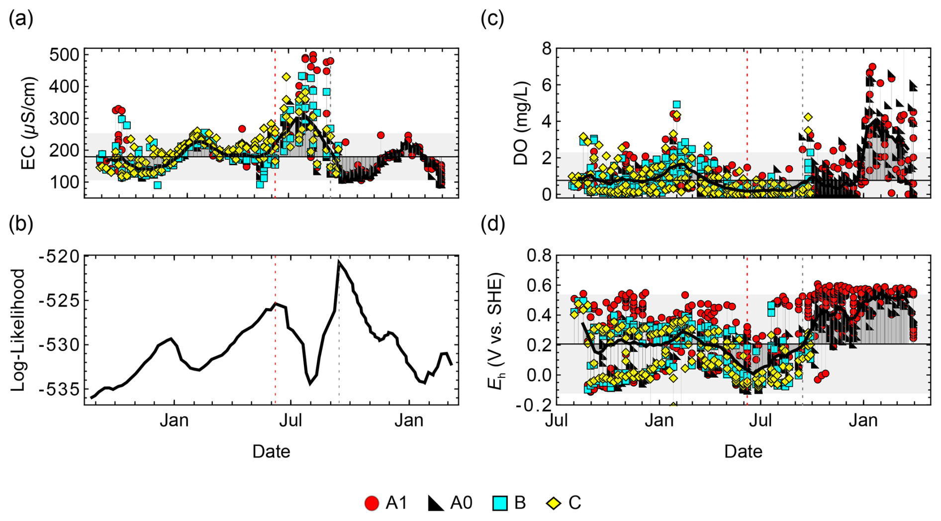
Figure 3 Disturbance-driven EC anomaly and likelihood-based change-point detection. (a) Weekly electrical conductivity (EC) at four monitoring sites (A1, A0, B, and C). (b) Log-likelihood profile of the two-segment Gaussian model applied to the EC time series at Site A1. (c) Dissolved oxygen (DO) time series. (d) Redox potential (E_h, vs. SHE) time series. Vertical dashed lines mark the operational change points adopted in the main text (red: disturbance onset associated with channel excavation; gray: transition from the EC amplification phase to the relaxation phase). Horizontal solid lines and shaded bands indicate the pooled pre-disturbance mean and mean ±1.96 SD range, respectively, calculated from all observations at all sites before completion of the excavation works (7 July 2022–7 June 2023).

To objectively identify the timing of disturbance onset, we applied change-point detection to the weekly EC time series using a two-segment Gaussian likelihood model, where each segment has its own mean and variance. For each candidate change point t_change, we computed the joint log-likelihood of the EC observations by fitting the model separately to the pre- and post-change segments. Because Sites B and C include substantial data gaps after the disturbance period, which can introduce spurious likelihood maxima, the change-point analysis was performed for Site A1 only (the primary reference site) and for the mean EC series across Sites A1 and A0, yielding consistent likelihood profiles (Fig. 3b). Local maxima in the likelihood profile were identified using the FindPeaks function in Wolfram Language (Mathematica 12.0; Wolfram Research, Champaign, IL, USA).

The global maximum of the likelihood corresponded to a change point separating the amplification phase from the subsequent relaxation phase (Fig. 3b). A second prominent peak coincided with the completion date of the channel excavation works (7 June 2023), indicating the transition from baseline conditions to the disturbance-driven EC increase. Because our primary objective is to define the onset of disturbance, we adopt this second peak as the operational change point and refer to the period prior to this date as the pre-disturbance regime and the subsequent period as the post-disturbance regime.

Dissolved oxygen (DO) tended to increase during the latter part of the post-disturbance regime relative to the same season in the previous year (Fig. 3c). This pattern may reflect multiple processes, including enhanced air–water gas exchange and vertical exchange associated with inflow/pumping events, as well as biological oxygen production and consumption. Over the same period, E_h exhibited an overall upward shift following the disturbance (Fig. 3d). Notably, during the pre-disturbance period E_h often showed vertical separation between surface and bottom waters, whereas this vertical divergence became less pronounced after the disturbance, consistent with enhanced vertical mixing.

Temperature, which can influence oxygen solubility and biological activity, showed typical seasonal cycles and vertical structure over the observation period, while pH ranged from 5.79 to 7.35 (mean 6.60) (Fig. A1).

3.3 Stability and breakdown of the ln[O₂]–E_h relationship

For the analyses below, DO was converted to molar concentration and used as a proxy for O₂ activity; ln [O₂] denotes the natural logarithm (base e). Because ln [O₂] is defined only for strictly positive values, DO records reported as 0.00 mg L⁻¹ were excluded from log-transformed analyses (see Methods for details).

During the pre-disturbance regime, a moderate positive relationship between ln [O₂] and E_h was consistently observed across sites (pooled regression: $E_{\mathrm{h}}=\mathrm{0.085}\ln \left[{\mathrm{O}}_{\mathrm{2}}\right]+\mathrm{1.18}$; adjusted R²=0.44; Fig. 4a). Site-specific slopes varied within a narrow range (0.072–0.104), and adjusted R² values were 0.46–0.52, with the highest value at Site A1 (Table A2). Despite strong seasonal variability in temperature and oxygen availability, the pre-disturbance data therefore exhibit a broadly consistent $\partial E_{\mathrm{h}}/\partial \ln \left[{\mathrm{O}}_{\mathrm{2}}\right]$ across sites, consistent with a relatively stable effective redox-reaction structure over this period.

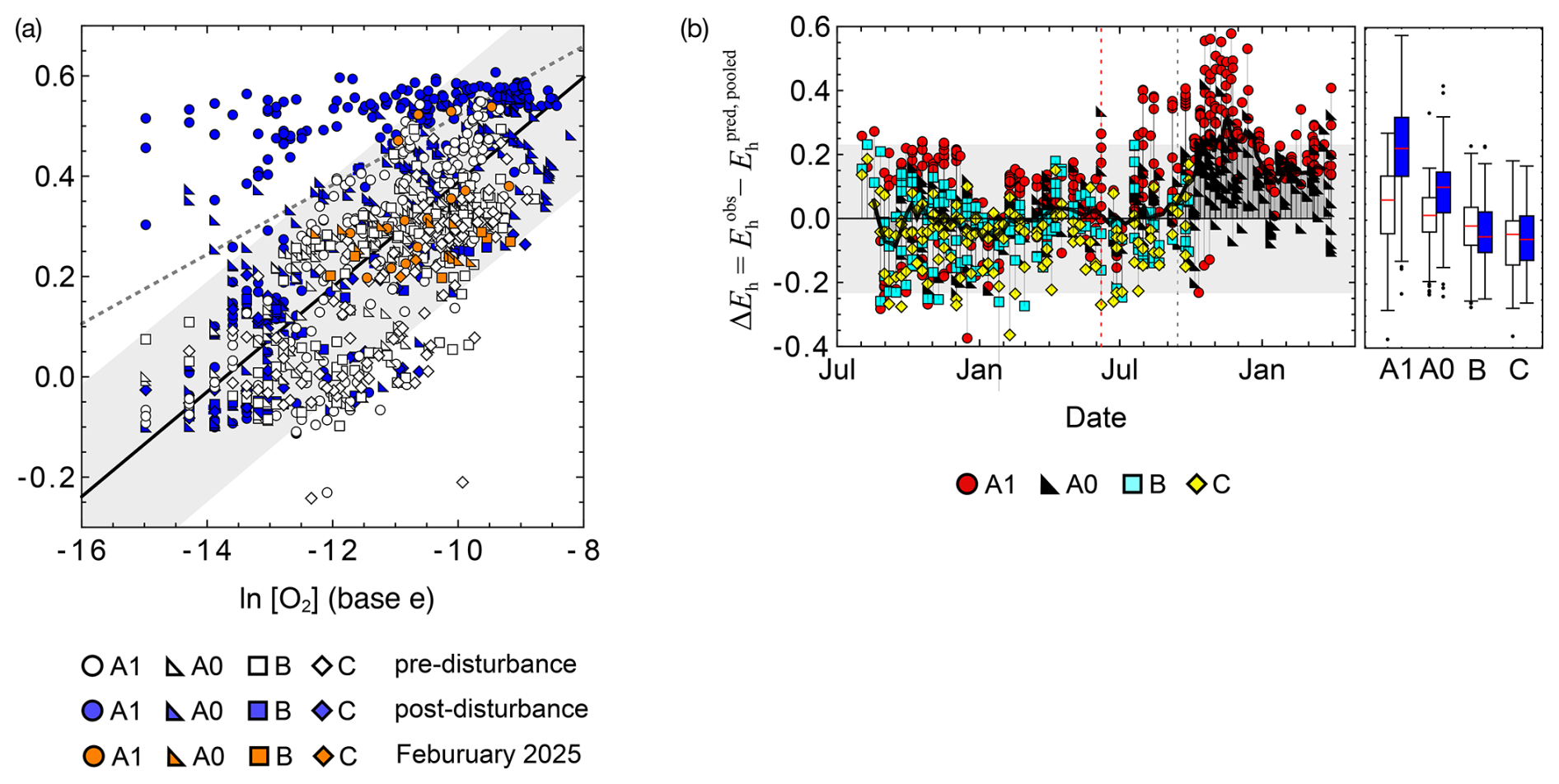
Figure 4 Disturbance-induced breakdown and recovery of the ln [O₂]–E_h relationship. (a) Relationship between E_h (V vs. SHE) and ln [O₂] (natural logarithm; base e) across Sites A1, A0, B, and C. Open symbols indicate the pre-disturbance regime and filled symbols indicate the post-disturbance regime; orange symbols denote the February 2025 follow-up vertical-profile survey. The solid and dashed lines show the pre- and post-disturbance regressions at Site A1, respectively. The shaded band represents the 95 % prediction interval of the pre-disturbance A1 regression. (b) Time series of residuals, $\mathrm{\Delta }{E}_{\mathrm{h}}=E_{\mathrm{h}}^{\mathrm{obs}}-E_{\mathrm{h}}^{\mathrm{pred},\mathrm{pooled}}$, where $E_{\mathrm{h}}^{\mathrm{pred},\mathrm{pooled}}$ was calculated from the pooled pre-disturbance regression. Vertical dashed lines mark the operational change points adopted in the main text (red: disturbance onset associated with channel excavation; gray: transition from the EC amplification phase to the relaxation phase). Boxplots summarize residual distributions for each site in the pre- (white) and post-disturbance (blue) regimes.

When the full observation period was considered, the ln [O₂]–E_h relationship at Site A1 weakened. The adjusted R² decreased by 0.153 relative to the pre-disturbance regression, indicating a loss of explanatory power. Site A1 is located closest to the inflow pathway and was most strongly affected by the sediment-mobilizing disturbance, suggesting a disturbance-driven modification of local redox conditions. Consistently, the slope at Site A1 decreased from 0.104 (pre-disturbance) to 0.067 (post-disturbance). Moreover, many post-disturbance observations at Site A1 lay above the 95 % prediction interval of the pre-disturbance regression, indicating a systematic elevation of E_h relative to the expected ln [O₂]–E_h relationship.

Enhanced vertical mixing after disturbance could reduce surface–bottom E_h separation and thereby shift the observed relationship. However, the persistence of elevated E_h even under low O₂ conditions suggests that the change is unlikely to be explained solely by physical mixing, indicating an altered sensitivity of E_h to oxygen availability following redox-network reconfiguration. Importantly, a follow-up vertical-profile survey in February 2025 showed that the pre-disturbance ln [O₂]–E_h relationship at Site A1 partially re-emerged (orange points in Fig. 4a), suggesting gradual recovery of the pre-disturbance redox structure.

To quantify deviations from the pre-disturbance system-level relationship, we computed residuals $\mathrm{\Delta }{E}_{\mathrm{h}}=E_{\mathrm{h}}^{\mathrm{obs}}-E_{\mathrm{h}}^{\mathrm{pred},\mathrm{pooled}}$, where $E_{\mathrm{h}}^{\mathrm{pred},\mathrm{pooled}}$ is the value predicted from the pooled pre-disturbance regression (Fig. 4b). Site A1 showed a pronounced positive shift in ΔE_h after disturbance, with the largest deviation occurring approximately three months after the EC peak. To compare pre- and post-disturbance residuals, we used a two-sample Student’s t-test when residuals were approximately normally distributed with no strong evidence of unequal variances (Sites A0 and C); otherwise we used the nonparametric Mann–Whitney U test (Sites A1 and B). Significant differences were detected at Sites A1 and A0 (p<0.05), whereas Sites B and C showed no significant difference, partly reflecting reduced sampling frequency after October due to logistical constraints.

4 Discussion

4.1 Mixed-potential interpretation of the observed slope breakdown

Field observations showed a relatively stable ln [O₂]–E_h relationship during the pre-disturbance regime across sites, followed by a disturbance-associated weakening and reorganization of the relationship, most clearly at Site A1 where sediment-laden inflow was strongest (Fig. 4a). Here we interpret these patterns in terms of mixed-potential control and clarify what is inferred from an observed ln [O₂]–E_h slope.

In the linearized mixed-potential framework (Eq. 5 with $x=\ln a_{{\mathrm{O}}_{\mathrm{2}}}$), the sensitivity $\partial E_{\mathrm{h}}/\partial \ln a_{{\mathrm{O}}_{\mathrm{2}}}$ reflects two components: a multi-reaction Nernst contribution through $\partial E_k/\partial \ln a_{{\mathrm{O}}_{\mathrm{2}}}$ and a contribution from changes in the relative conductance weights of the reactions that collectively form the mixed potential. Importantly, an approximately constant ln [O₂]–E_h slope does not require that E_h be controlled by a single redox couple; it is also consistent with a multi-reaction mixed potential whose effective set of contributing reactions and their relative weights remain approximately invariant over the range of oxygen variability. Conversely, a change in slope indicates that the effective reaction set and/or its relative weighting has been reorganized, i.e., oxygen-related electron-transfer pathways have been reweighted relative to other concurrent pathways.

The ln [O₂]–E_h relationship at Site A1 can be translated into mixed-potential terms as follows. A weakened slope suggests a reduced relative weighting of oxygen-coupled interfacial pathways (or an increased contribution of competing pathways), so that changes in oxygen activity produce a smaller shift in the conductance-weighted balance that sets E_mix. A systematic positive shift in ΔE_h at a given ln [O₂] indicates an upward displacement of the mixed-potential baseline, consistent with a reweighting and/or replacement of the effective reaction set toward higher equilibrium-potential contributions under otherwise comparable oxygen levels. The lagged peak in ΔE_h after the EC anomaly relaxed implies that this reorganization persisted beyond the transient ionic-strength/turbidity perturbation, pointing to a slowly evolving internal state that continued to modulate the reaction weights. The partial recovery observed in February 2025 is consistent with gradual re-establishment of the pre-disturbance effective reaction set and its relative weights.

Within Eq. (5), such slow evolution can act through gradual changes in partial polarization conductances and thus in reaction weights, for example via sediment-associated redox buffering, evolving availability of redox-active solutes, and progressive re-establishment of pre-disturbance reaction pathways (Herbel et al., 2007). In the next section, we examine this possibility using a minimal model that isolates the role of slowly varying reaction weights.

We note that electrode-related effects cannot be fully excluded because routine external calibration was not performed. However, the shift showed coherent timing with the documented disturbance, a spatial structure (A1 > A0), and partial recovery in the follow-up profile survey. These features are difficult to reconcile with a simple monotonic sensor-drift scenario and instead support our interpretation that the observed changes primarily reflect system-level reorganization of the interfacial redox processes supplying electrons to the electrode.

4.2 A minimal timescale-separation model for delayed slope changes

Building on the mixed-potential interpretation above, we introduce a minimal timescale-separation model to illustrate how a change in the apparent ln [O₂]–E_h slope can emerge with a delay relative to a fast physical disturbance signature. The model reduces Eq. (4) to two effective branches: an oxygen-sensitive branch and an oxygen-insensitive high-potential branch, whose relative weight varies slowly in time. This toy model is intended to demonstrate mechanistic plausibility (timescale-separated re-weighting under mixed-potential control), rather than to simulate the observed patterns.

We decompose the dynamics into (i) fast oxygen forcing, representing seasonal and short-period fluctuations in O₂ (Fig. 5a), and (ii) a slow internal state variable, s(t), representing a pulse-like disturbance and its lingering effect that controls how strongly oxygen-dependent reactions contribute to the mixed potential (Fig. 5b). Here, s denotes a latent (unobserved) state variable representing slow changes in the near-electrode redox environment that modulate the relative contributions of interfacial reactions (i.e., G_k), rather than a directly measured chemical species.

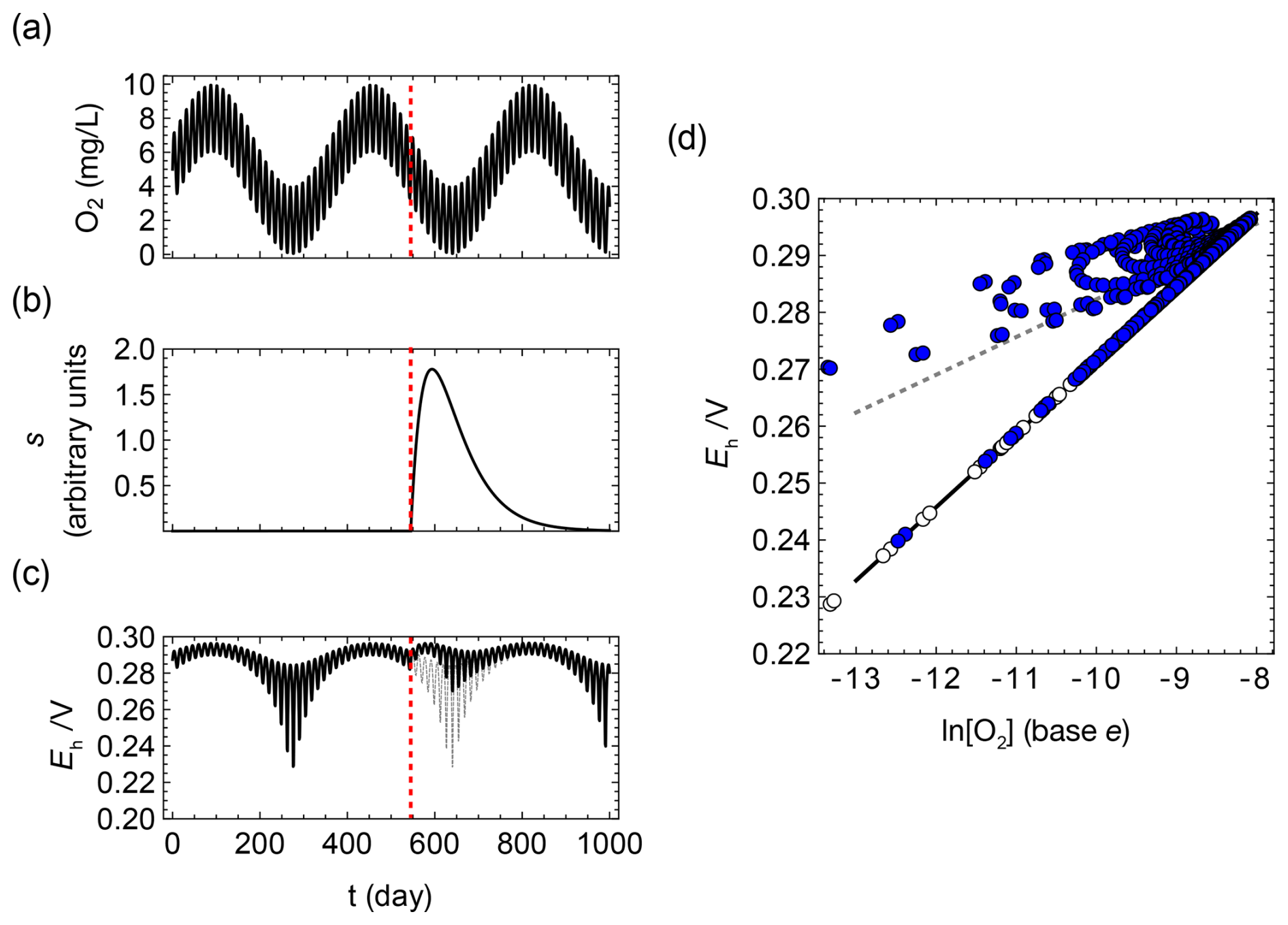
Figure 5 Conceptual two-branch mixed-potential simulation illustrating delayed changes in the apparent $\partial E_{\mathrm{h}}/\partial \ln \left[{\mathrm{O}}_{\mathrm{2}}\right]$ following a pulse-like disturbance. (a) Prescribed O₂(t) forcing composed of seasonal and short-period fluctuations. (b) A slow latent internal state s(t) (proxy for gradual reconfiguration of the near-electrode redox environment) responding to a pulse forcing applied at t=t_p (red dashed line) and relaxing with timescale τ. (c) Simulated E_h(t) under mixed-potential control. Black: with disturbance-driven evolution of s(t); gray: counterfactual trajectory without disturbance (u(t)≡0). (d) Phase plot of E_h versus ln [O₂]. Open circles indicate the pre-disturbance period (t<t_p) and filled circles indicate the post-disturbance period (t≥t_p). Solid and dotted lines show separate linear regressions for the pre- and post-disturbance periods, respectively.

The E_h dynamics are represented as follows:

$$\begin{array}{}\text{(7)}& \begin{array}{rl}{E}_{\mathrm{h}}\left(t\right)& =(\mathrm{1}-w(s\left)\right)E_{{\mathrm{O}}_{\mathrm{2}}}\left(t\right)+w\left(s\right)E_{\mathrm{H}},\\ w\left(s\right)& ={\displaystyle \frac{G_{\mathrm{H}}\left(s\right)}{G_{{\mathrm{O}}_{\mathrm{2}}}+G_{\mathrm{H}}\left(s\right)}},\end{array}\end{array}$$

where $E_{{\mathrm{O}}_{\mathrm{2}}}\left(t\right)$ follows a Nernstian dependence,

$$\begin{array}{}\text{(8)}& E_{{\mathrm{O}}_{\mathrm{2}}}\left(t\right)=E_{{\mathrm{O}}_{\mathrm{2}}}^{\mathrm{0}}+\mathit{\gamma }\ln \left[{\mathrm{O}}_{\mathrm{2}}\right(t\left)\right],\end{array}$$

whereas E_H is assumed insensitive to oxygen on the timescale of interest. The weight factor w(s) increases with a slow latent state s(t) (e.g., through a logistic dependence of G_H on s), so that larger s increases the contribution of the high-potential branch (the specific functional form and parameters are given in the Appendix B).

The slow variable evolves as

$$\begin{array}{}\text{(9)}& {\displaystyle \frac{ds}{dt}}=-{\displaystyle \frac{s-s_{\mathrm{0}}}{\mathit{\tau }}}+u\left(t\right),\end{array}$$

where u(t) represents a pulse-like disturbance forcing and τ is a relaxation timescale that is long relative to oxygen fluctuations.

This minimal structure yields two key behaviors that mirror our field patterns (Fig. 5c, d). First, the instantaneous slope with respect to oxygen is

$$\begin{array}{}\text{(10)}& {\displaystyle \frac{\partial E_{\mathrm{h}}}{\partial \ln \left[{\mathrm{O}}_{\mathrm{2}}\right]}}=\mathit{\gamma }(\mathrm{1}-w(s\left)\right),\end{array}$$

so that an increase in w(s) produces a reduced apparent $\partial E_{\mathrm{h}}/\partial \ln \left[{\mathrm{O}}_{\mathrm{2}}\right]$ slope (Fig. 5d). Second, when w(s) becomes large, E_h can remain high even when O₂ is low (Fig. 5b, c), because the high-potential branch dominates the mixed potential. Because s evolves slowly, both the slope reduction and the elevated-E_h residuals can persist and peak after fast disturbance indicators (such as EC) have subsided. Thus, the delayed emergence of the A1 residual shift is consistent with a gradual reconfiguration of the effective redox reaction network.

4.3 Practical implications for monitoring shallow-water redox dynamics

DO is a common target of routine monitoring in aquatic systems, partly because it is directly linked to key ecological processes such as organic-matter degradation and community structure (Bastviken et al., 2004; Connolly et al., 2004; Wang et al., 2008; Franklin, 2014). In contrast, E_h has been used far more selectively, despite the growing availability of robust, field-deployable electrodes suitable for long-term deployment (Vorenhout et al., 2004; Wang et al., 2022). Our results show that neither DO nor E_h alone provides an indicator of system-level redox-network stability, whereas their joint behavior can provide a compact diagnostic of redox-structural change.

In this study, we propose two complementary metrics based on the co-located 21-month DO and E_h measurements. First, the stability (or breakdown) of the ln [O₂]–E_h slope serves as an indicator of whether the effective reaction set contributing to the mixed potential remains structurally invariant. Second, baseline-referenced residuals (here, $\mathrm{\Delta }{E}_{\mathrm{h}}=E_{\mathrm{h}}^{\mathrm{obs}}-E_{\mathrm{h}}^{\mathrm{pred}}$, with $E_{\mathrm{h}}^{\mathrm{pred}}$ computed from the pooled pre-disturbance regression; Fig. 4b) provide a practical measure of departures from the system-level relationship. Together, these metrics provide a practical way to identify departures from a site-specific DO–E_hbaseline that are consistent with disturbance-induced changes in effective redox conditions and subsequent recovery, using instrumentation that is already routinely deployed.

At the same time, the mixed-potential nature of E_h imposes clear limits on interpretation. Because multiple combinations of interfacial pathways can yield the same electrode potential, co-monitoring DO and E_h cannot identify the dominant redox couple(s), resolve aqueous speciation, or quantify individual reaction fluxes without complementary measurements of redox-active species. Furthermore, the proposed DO–E_h approach is not intended to imply that dissolved oxygen universally controls E_h. Its applicability is limited to settings where oxygen is present and variable enough for a DO–E_h relationship to be evaluated. In oxygen-depleted or strongly reducing environments, other redox-active systems may dominate the mixed potential, and complementary measurements of redox-active species would be needed to identify the underlying processes.

Because the present study was conducted in a small constructed pond, generalization to larger and more complex aquatic systems should be made cautiously. In lakes, rivers, and reservoirs, stratification, advective transport, sediment–water exchange, lateral inputs, and spatial heterogeneity may produce multiple DO–E_h regimes within the same system. Application of the proposed approach to such environments would require site-specific baseline characterization, careful spatial design of co-located DO and E_h measurements, and, where possible, complementary measurements of redox-active species.

DO–E_h co-monitoring is therefore best viewed not as a substitute for comprehensive geochemical characterization, but as a low-cost screening-level approach for detecting departures from a site-specific DO–E_h baseline that may indicate changes in effective redox conditions or in the relative contributions of redox-active processes.

5 Conclusions

We revisited field-measured E_h as a mixed potential and asked what mechanistic insight can be extracted from its relationship with a single species, here dissolved oxygen. In a linearized mixed-potential framework, an approximately constant log-linear E_h sensitivity to ln [O₂] can arise when the effective set of interfacial reactions contributing to E_h and their relative polarization conductances remain approximately invariant; such behavior therefore does not require dominance by a single redox couple. Applying this interpretation to a 21-month multi-site time series (July 2022 to March 2024) from a constructed pond, we found that the pre-disturbance ln [O₂]–E_h slope was relatively stable across sites, whereas the site most affected by sediment mobilization (A1) showed a marked weakening and reorganization of the relationship after disturbance. Residuals relative to the pooled pre-disturbance baseline exhibited a pronounced positive shift at A1, peaking after the EC anomaly had largely relaxed, and follow-up vertical profiles in February 2025 indicated partial recovery of the pre-disturbance relationship. Together, these results support the use of the ln [O₂]–E_h slope and baseline residuals as practical, screening-level indicators of departures from a site-specific redox baseline derived from co-located sensor measurements. These departures are consistent with disturbance-driven changes in effective redox conditions, although complementary measurements of redox-active species would be needed to resolve the underlying redox processes and dominant redox couples.

Appendix A: Linearization-based derivation of the mixed potential

For each reaction k, we define the potential E_k at which the partial current vanishes by i_k(E_k)=0. The quantity E_k represents the potential at which electrochemical equilibrium is established between the redox couple involved in reaction k and the electron bath of the electrode. For partial reactions whose current–potential response is evaluated near E_k, the partial current i_k(E) can be expanded in a Taylor series around E_k:

$$\begin{array}{}\text{(A1)}& i_k\left(E\right)=i_k\left(E_k\right)+{\left.{\displaystyle \frac{\mathrm{d}{i}_k}{\mathrm{d}E}}\right|}_{E=E_k}(E-E_k)+\mathcal{O}\left(\right(E-E_k{)}^{\mathrm{2}}).\end{array}$$

Since i_k(E_k)=0 by definition, retaining only the linear term yields

$$\begin{array}{}\text{(A2)}& i_k\left(E\right)\simeq G_k(E-E_k)\end{array}$$

where

$$\begin{array}{}\text{(A3)}& G_k\equiv {\left.{\displaystyle \frac{d{i}_k}{dE}}\right|}_{E=E_k}\end{array}$$

is the local polarization conductance of partial reaction k, defined as the slope of the partial current–potential response near the equilibrium point. Equivalently, it is the reciprocal of the local polarization resistance for that partial reaction. Substituting Eq. (A2) into Eq. (1) gives

$$\begin{array}{}\text{(A4)}& \sum _k{i}_k\left(E\right)\simeq \sum _k{G}_k(E-E_k).\end{array}$$

For the subset of partial reactions that contribute appreciably to the mixed potential, we approximate the current–potential response near E_mix by the local linear expansion around E_k. This approximation is most appropriate when the relevant overpotentials on the Pt electrode remain within a near-linear polarization range. Evaluating Eq. (A4) at E=E_mix and imposing the zero-current condition gives

$$\begin{array}{}\text{(A5)}& \sum _k{G}_k(E_{\mathrm{mix}}-E_k)=\mathrm{0}.\end{array}$$

Rearranging this expression yields

$$\begin{array}{}\text{(A6)}& E_{\mathrm{mix}}={\displaystyle \frac{{\sum }_k{G}_k{E}_k}{{\sum }_k{G}_k}},\end{array}$$

showing that, in the small-overpotential limit, the mixed potential is given by a conductance-weighted average of the equilibrium potentials E_k of the individual reactions.

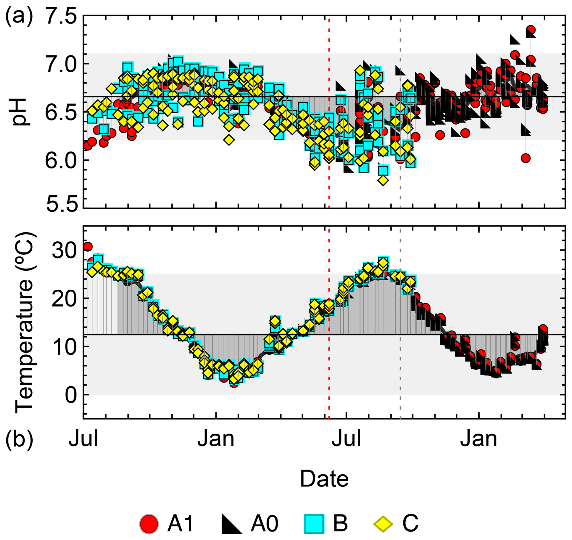
Figure A1 Time series of (a) pH and (b) water temperature measured in situ at the four monitoring sites (A1, A0, B, and C) from July 2022 to March 2024. Symbols show weekly measurements at different depths at each site. Vertical dashed lines mark the operational change points adopted in the main text (red: disturbance onset associated with channel excavation; gray: transition from the EC amplification phase to the relaxation phase). Solid lines and shaded bands indicate the mean and mean ± 1.96 SD range during pre-disturbance regime calculated from all sites.

Table A1 Specifications of instruments and sensors used for in situ monitoring.

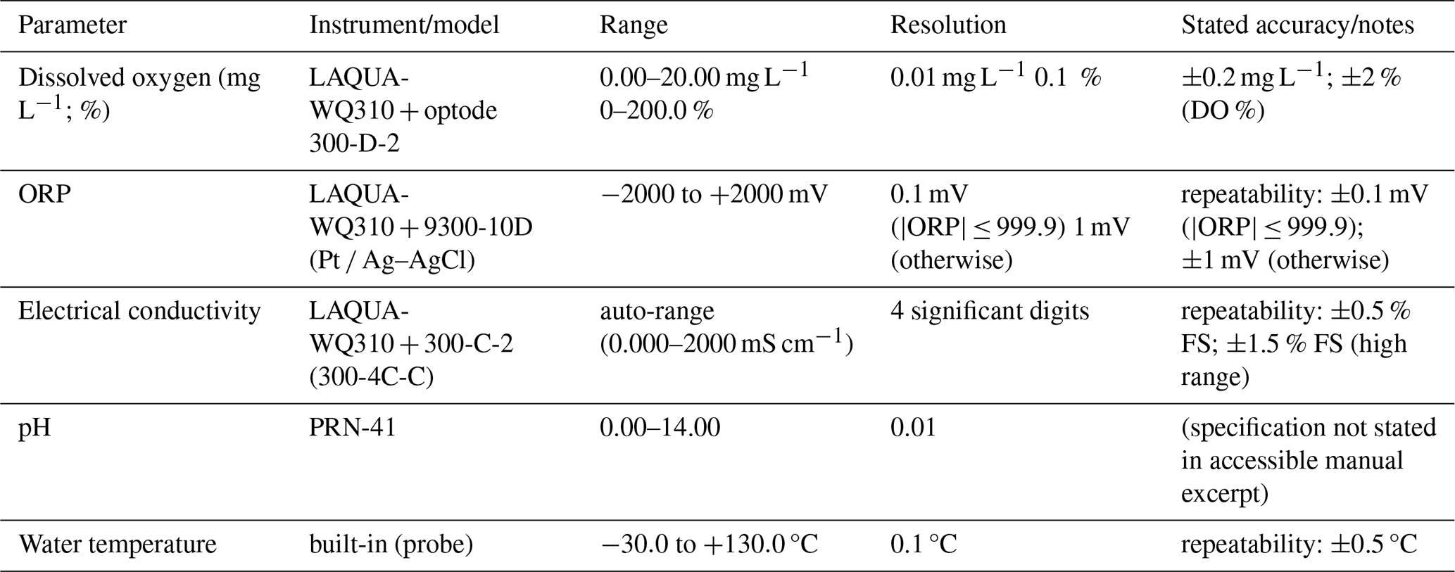
Table A2 Linear regression summaries for the relationship between E_h (V vs. SHE) and ln [O₂] (natural logarithm, base e). We approximated the activity of O₂ by its molar concentration; therefore, data with DO =0 were excluded from regression because ln [O₂] is undefined. “All sites” indicates pooled data across sites. The pre-disturbance regime was defined based on the EC change-point analysis (see main text).

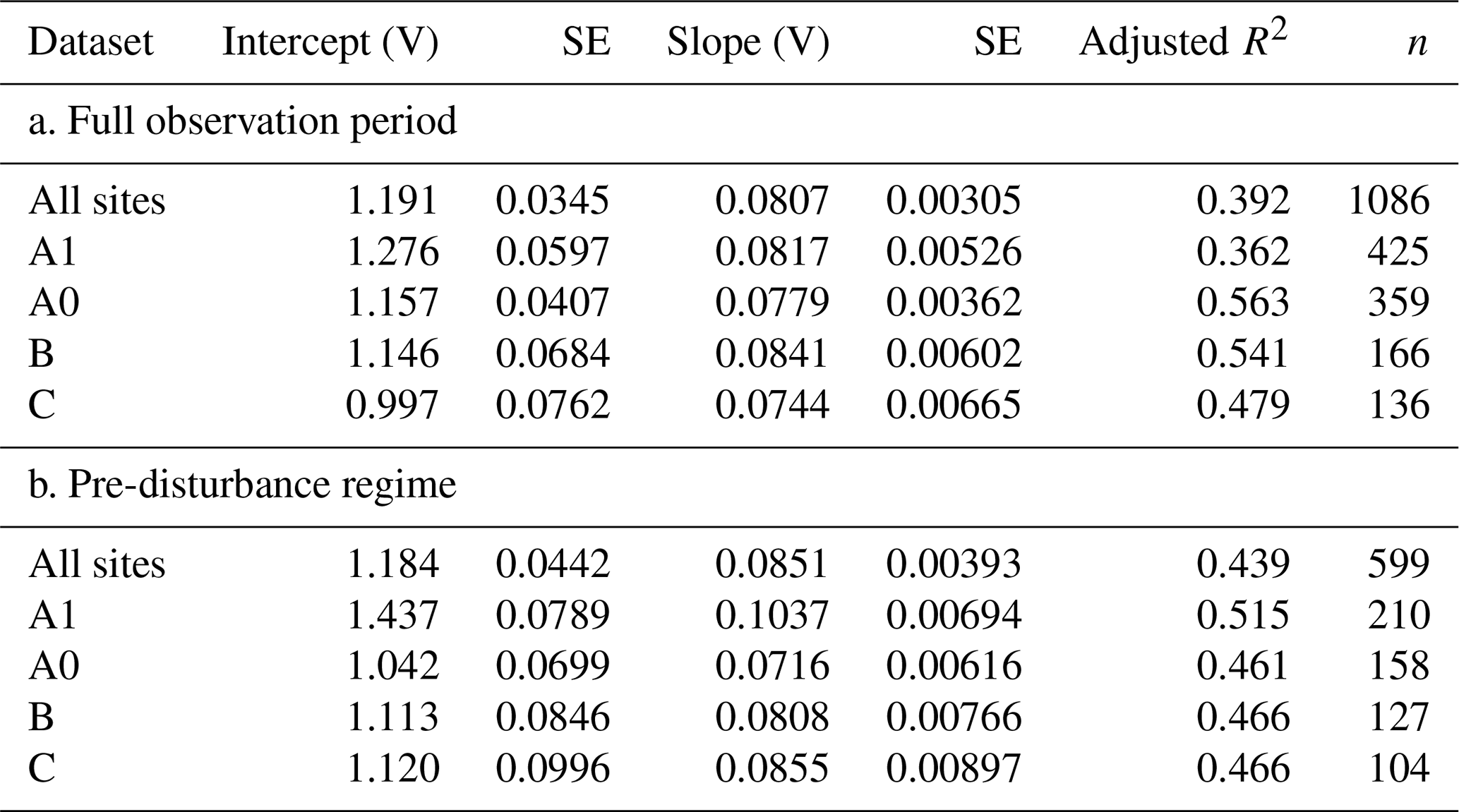
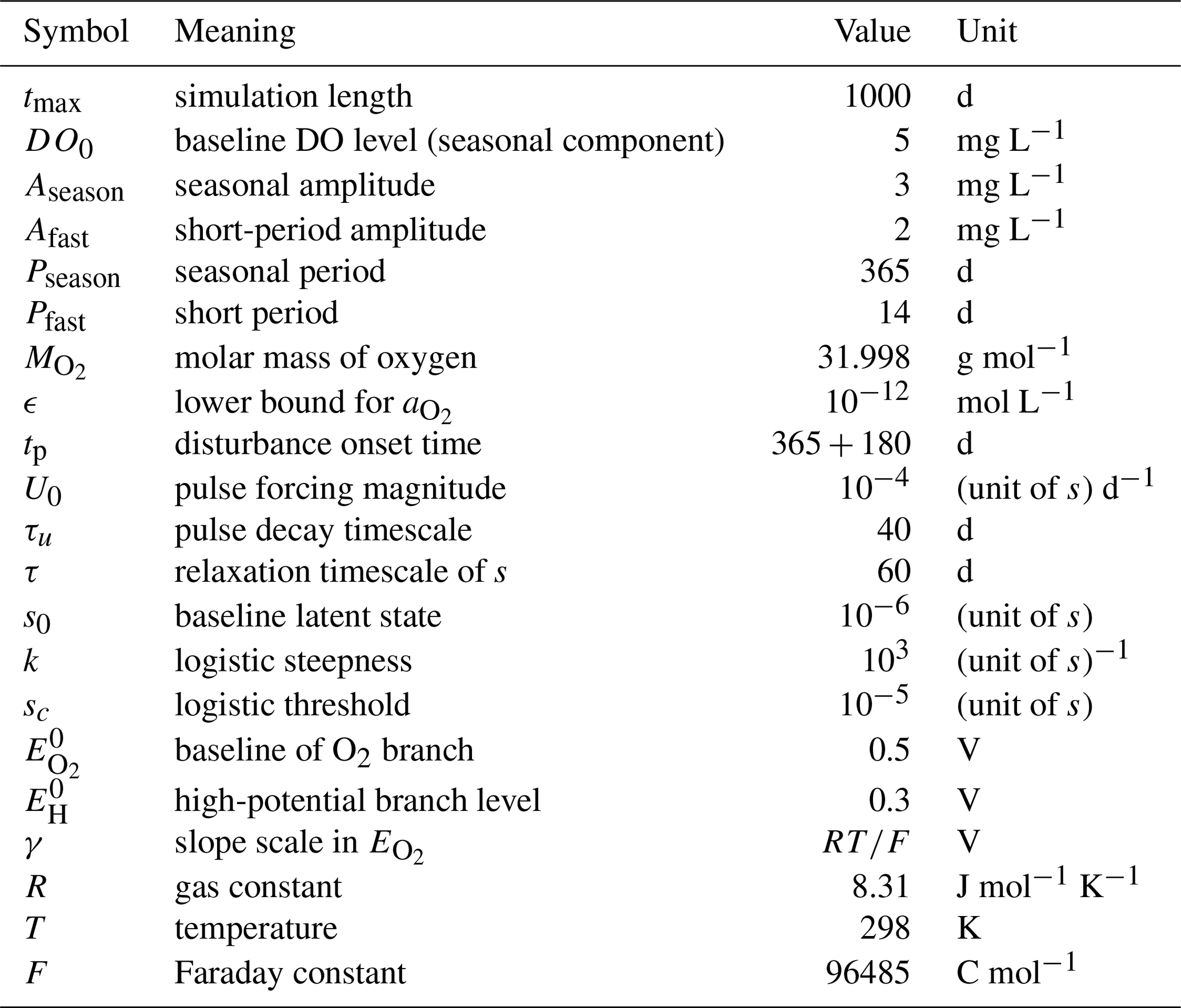
Table A3 Parameter values used in the minimal timescale-separation simulation (Fig. 5).

Appendix B: Minimal timescale-separation model

B1 Model definition

We constructed a two-branch mixed-potential toy model to demonstrate how an apparent change in the ln [O₂]–E_h slope can be delayed relative to a fast disturbance signature. The model is intended to show mechanistic plausibility (timescale-separated re-weighting under mixed-potential control), rather than to reproduce the observed magnitudes.

B1.1 Oxygen forcing

We prescribed an oxygen-activity proxy $a_{{\mathrm{O}}_{\mathrm{2}}}\left(t\right)$ as the sum of seasonal (period P_season) and short-period (period P_fast) components. The forcing was constructed in concentration units by converting an equivalent DO signal (mg L⁻¹) to mol L⁻¹ using the molar mass of O₂ ($M_{{\mathrm{O}}_{\mathrm{2}}}$):

$$\begin{array}{}\text{(B1)}& a_{{\mathrm{O}}_{\mathrm{2}}}\left(t\right)=max\mathit{\{}\mathit{ϵ},a_{\mathrm{season}}(t)+a_{\mathrm{fast}}(t\left)\mathit{\right\}},\end{array}$$

where

$$\begin{array}{}\text{(B2)}& \begin{array}{rl}& a_{\mathrm{season}}\left(t\right)={\mathrm{10}}^{-\mathrm{3}}{\displaystyle \frac{{\mathrm{DO}}_{\mathrm{0}}+A_{\mathrm{season}}\sin (\mathrm{2}\mathit{\pi }t/P_{\mathrm{season}})}{M_{{\mathrm{O}}_{\mathrm{2}}}}},\\ & a_{\mathrm{fast}}\left(t\right)={\mathrm{10}}^{-\mathrm{3}}{\displaystyle \frac{A_{\mathrm{fast}}\sin (\mathrm{2}\mathit{\pi }t/P_{\mathrm{fast}})}{M_{{\mathrm{O}}_{\mathrm{2}}}}}.\end{array}\end{array}$$

We imposed a lower bound ϵ to avoid undefined values in $\ln a_{{\mathrm{O}}_{\mathrm{2}}}$.

B1.2 Slow latent state with pulse-like forcing

A slow latent state s(t) evolves as

$$\begin{array}{}\text{(B3)}& {\displaystyle \frac{\mathrm{d}s}{\mathrm{d}t}}=-{\displaystyle \frac{s-s_{\mathrm{0}}}{\mathit{\tau }}}+u\left(t\right),s\left(\mathrm{0}\right)=s_{\mathrm{0}},\end{array}$$

where the disturbance forcing is

$$\begin{array}{}\text{(B4)}& u\left(t\right)=U_{\mathrm{0}}\exp \left(-{\displaystyle \frac{t-t_{\mathrm{p}}}{{\mathit{\tau }}_u}}\right)H(t-t_{\mathrm{p}}),\end{array}$$

and H(⋅) denotes the Heaviside step function.

B1.3 Reaction weight and two-branch mixed potential

We mapped s(t) to the effective reaction weight using a logistic function,

$$\begin{array}{}\text{(B5)}& w\left(s\right)={\displaystyle \frac{\mathrm{1}}{\mathrm{1}+\exp \mathit{\{}-k(s-s_c\left)\mathit{\right\}}}}.\end{array}$$

The modeled redox potential is a weighted mixture of an oxygen-sensitive branch and an oxygen-insensitive high-potential branch:

$$\begin{array}{}\text{(B6)}& E_{\mathrm{h}}\left(t\right)=(\mathrm{1}-w(s\left(t\right)\left)\right)E_{{\mathrm{O}}_{\mathrm{2}}}\left(t\right)+w\left(s\right(t\left)\right)E_{\mathrm{H}}^{\mathrm{0}}.\end{array}$$

The oxygen-sensitive branch follows a Nernst-type dependence,

$$\begin{array}{}\text{(B7)}& E_{{\mathrm{O}}_{\mathrm{2}}}\left(t\right)=E_{{\mathrm{O}}_{\mathrm{2}}}^{\mathrm{0}}+\mathit{\gamma }\ln a_{{\mathrm{O}}_{\mathrm{2}}}\left(t\right),\end{array}$$

where γ is treated as a slope-scale parameter (set to $RT/F$ in our demonstration run; Table A3). A no-perturbation reference trajectory was obtained by fixing the weight at w(s₀):

$$\begin{array}{}\text{(B8)}& E_{\mathrm{h}}^{\mathrm{wop}}\left(t\right)=(\mathrm{1}-w(s_{\mathrm{0}}\left)\right)E_{{\mathrm{O}}_{\mathrm{2}}}\left(t\right)+w\left(s_{\mathrm{0}}\right)E_{\mathrm{H}}^{\mathrm{0}}.\end{array}$$

B1.4 Instantaneous slope

Because E_h is affine in $\ln a_{{\mathrm{O}}_{\mathrm{2}}}$ for fixed w, the instantaneous slope is

$$\begin{array}{}\text{(B9)}& {\displaystyle \frac{\partial E_{\mathrm{h}}}{\partial \ln a_{{\mathrm{O}}_{\mathrm{2}}}}}=\mathit{\gamma }(\mathrm{1}-w(s\left(t\right)\left)\right),\end{array}$$

so that an increase in w yields an apparent weakening of the ln [O₂]–E_h sensitivity.

B2 Numerics and parameters

We solved the ODE for s(t) using NDSolve over $t\in [\mathrm{0},t_{max}]$ and computed E_h(t) from the closed-form expressions above. The logistic weight w(s) was evaluated along the numerical trajectory s(t). All parameter values used for the demonstration run are listed in Table A3.