Direct estimation of wildfire emissions at high latitudes from combined polar orbiter FRP and Sentinel-5P CO data

High Latitude (HL) landscape fires are an important source of greenhouse gases and aerosols, with growing significance under rapid anthropogenic climate change-induced warming. Current fire emission inventories are mostly “bottom-up” in nature; combining, or relying on linear regressions between, satellite remote sensing data and process-based model outputs. However, these methods rely on uncertainties surrounding fuel load and combustion completeness. Here, we adapt the “top-down” Fire Radiative Energy Emission (FREM) approach for HL fires (HLFREM), linking Fire Radiative Energy (FRE) directly to emissions via coefficients derived solely from satellite observations. We derive biome-specific emission coefficients by combining Fire Radiative Power (FRP) from GFAS v1.4 with TROPOMI Total Column Carbon Monoxide plume observations, for the HL's four most fire-prone biomes; Deciduous and Evergreen Needleleaf Forests, Grasslands, and Shrublands. By applying these coefficients to daily GFAS v1.2 FRE totals (2003–2024), we estimate CO and total carbon emissions across the HL using HLFREM. HLFREM-derived CO emissions were found to be in good temporal and spatial agreement, but smaller in emission totals than other widely used inventories (GFAS v1.2 and GFEDv4.1s) in forested biomes, as well as with the MODIS-based FEER approach, with annual average differences of 54 % to 62 % smaller for Deciduous Needleleaf Forests, and 59 % to 70 % smaller for Evergreen Needleleaf forests. For Shrublands and Grassland biomes, HLFREM estimates are 65 %–75 % and 71 %–85 % lower respectively. Total carbon emissions, using Emission Factors, were found to show consistent patterns with CO across all biomes.

1 Introduction

Landscape fire is Earth's largest natural disturbance agent, burning, according to the latest satellite-derived datasets, an average of approximately 5.5 % of Earth's land surface annually (Chen et al., 2023). These landscape fires greatly affect ecology, land carbon stores, atmospheric composition, air quality, and human health. The true magnitude of these effects may even be higher than currently estimated, due to satellite-based burned area mapping often missing many of the highly-numerous smaller burns that together make up a significant fraction of total global burned area (Ramo et al., 2021), even when adjusted for some of this low bias (Chen et al., 2023).

Satellite data indicates that vegetation fires are extensive across every vegetated continent apart from Antarctica, including even High Latitude (HL, ≥60° N) areas (Jones et al., 2022) up to 75° N (Masrur et al., 2018). Such HL burns include so-called “Arctic-fires” (i.e. fires taking place at latitudes above 66° N) which are of increasing interest, in part because evidence suggests an increase in both their frequency and magnitude; potentially driven by the rapid warming of Earth's climate occurring in more northerly regions (McCarty et al., 2021). These Arctic-fires, for example those in Siberia in 2020 and 2021 (Kharuk et al., 2021; Liu et al., 2022) can be seen as an extension of the wider northern (i.e. Boreal) regions' fire activity (McCarty et al., 2021), which is itself apparently increasing (Masrur et al., 2018). This is most commonly attributed to lengthening of the “fire season”, the period of the year when vegetation, litter and/or organic soils are sufficiently warm and dry for significant landscape fires to ignite and spread.

Frequent lightning, and the extensive uninterrupted fuel (primarily forest) cover, promotes fire in many HL areas; with certain tree species having evolved to include fire as part of their reproductive cycle (Hodges et al., 2021; Hutto, 2008). Such adaptations and their regionally varying occurrence in HL regions are apparently behind many of the spatial differences seen in certain remotely sensed fire signatures (Rogers et al., 2015; Wooster and Zhang, 2004). Because many of the forests of the HL regions ultimately require fire to thrive, wildfires are often left to burn without intervention if they pose little-to-no threat to humans or property. However, there is a concern that the massive stores of ground carbon contained in the underlying peat and organic soils of northern regions, some of which have remained frozen for millennia, may also be becoming more accessible to fire (Davidson and Janssens, 2006; Turetsky et al., 2002). Burning of these carbon stores results in net greenhouse gases (GHGs) emissions that are unreplaced by photosynthetic carbon reassimilation (i.e. vegetation regrowth) on the decades-to-century time-scales typical of forest recovery (Friedlingstein et al., 2021). Quantifying HL fire activity and any trends in its nature is therefore valuable for understanding fires contribution to net atmospheric greenhouse gas concentrations (Mekonnen et al., 2022), as well as for issues such as air quality (Warneke et al., 2023).

Calculating the amount of land carbon (i.e. live vegetation, litter and, organic soil) consumed by fire, including in HL fires, as well as emissions of Carbon Monoxide (CO) and other GHGs, reactive gases, and aerosols, typically involves a so-called “bottom-up” calculation (Crutzen and Andreae, 1990), with the most modern implementations combining modelling and satellite-derived datasets (Ichoku and Ellison, 2014; Kaiser et al., 2012; van der Werf et al., 2010, 2017). The most common implementation, the Global Fire Emission Database (GFED, Randerson et al., 2017), is driven by satellite-derived measures of burned area, but is still classed as an “indirect” approach since it relies heavily on mathematical models and/or in-situ assessments for the fuel load and combustion completeness parameters that remain subject to significant uncertainty at any particular location (Reid et al., 2009). An alternative satellite-based “direct” approach relies on Fire Radiative Power (FRP) measures rather than burned area, with FRP representing the radiant energy released per unit time by the combustion process. These FRP data can be time-integrated to estimate the Fire Radiative Energy (FRE) released by the burn, which then links to total fuel consumption (Roberts et al., 2005; Wooster et al., 2005, 2015). FRP-based approaches avoid the need for assumed or modelled fuel load and combustion completeness terms (Kasischke and Penner, 2004), but are not always fully independent of the burned area-based methods since the necessary “FRP-to-fuel consumption” conversion coefficients are themselves often derived from correlations and regressions made between FRE datasets and the outputs of the more indirect burned area-based approach; such as with the Global Fire Assimilation System (GFAS, Kaiser et al., 2012). Alternatively, such conversion coefficients have been based on limited numbers of direct comparisons between FRE and fuel consumption, but in mostly small-scale or laboratory burns which may not accurately represent the dynamics of real landscape scale fires, nor the full characteristics of the FRP measurements made from Earth orbit (Freeborn et al., 2008; Nguyen and Wooster, 2020; Wooster et al., 2005).

More recently, even more direct “top-down” FRP-based emissions assessment methodologies have emerged; now relating smoke emissions directly to the observed FRP of landscape fires. Their uniqueness is that, in order to reduce the aforementioned issues and embedded assumptions that arise when using satellite-derived FRE totals with “FRP-to-fuel consumption” conversion coefficients, these new approaches use direct satellite-based measurements of fire emissions and FRP, via a set of “matchup fires”, to generate a set of landscape-fire “emissions coefficients” that can be used to generate smoke emissions estimates directly from all other FRP observations of the area.

These more direct assessments have included both airborne observations of landscape fire and their associated emitted smoke species (Hayden et al., 2022; Owsley-Brown et al., 2024; Stockwell et al., 2022) as well as satellite-based observations (Adams et al., 2019; Griffin et al., 2024; Mebust et al., 2011); calculating emission coefficients of observed landscape fires categorised in terms of field campaign and land cover type (Griffin et al., 2024).

One of the most recent such approaches, termed the Fire Radiative Energy Emissions (FREM) method (Mota and Wooster, 2018; Nguyen and Wooster, 2020), derives these emissions coefficients directly from geostationary satellite FRE estimates and matching smoke plume Earth observation data (Fisher et al., 2020; Mota and Wooster, 2018; Nguyen and Wooster, 2020). Emissions coefficients derived in this way are appropriate to real landscape fires of all sizes, minimally reliant on any assumptions, and appropriate to apply to further satellite FRE data to convert them into smoke emissions estimates (Nguyen et al., 2023). Thus far, the FREM approach has relied on geostationary satellites to provide the high imaging frequency FRP data with which to accurately estimate FRE via temporal integration. Observations made by equatorial orbit geostationary satellites are, however, of mostly poor quality at high latitudes. However, whilst FRP-to-FRE calculations based on polar orbiting satellite data can be challenging at lower latitude fires due to the limited temporal sampling of FRP provided (Mota and Wooster, 2018), at higher latitudes orbital convergence generally provides far more polar-orbiting based estimates of FRP per day (Fig. 1).

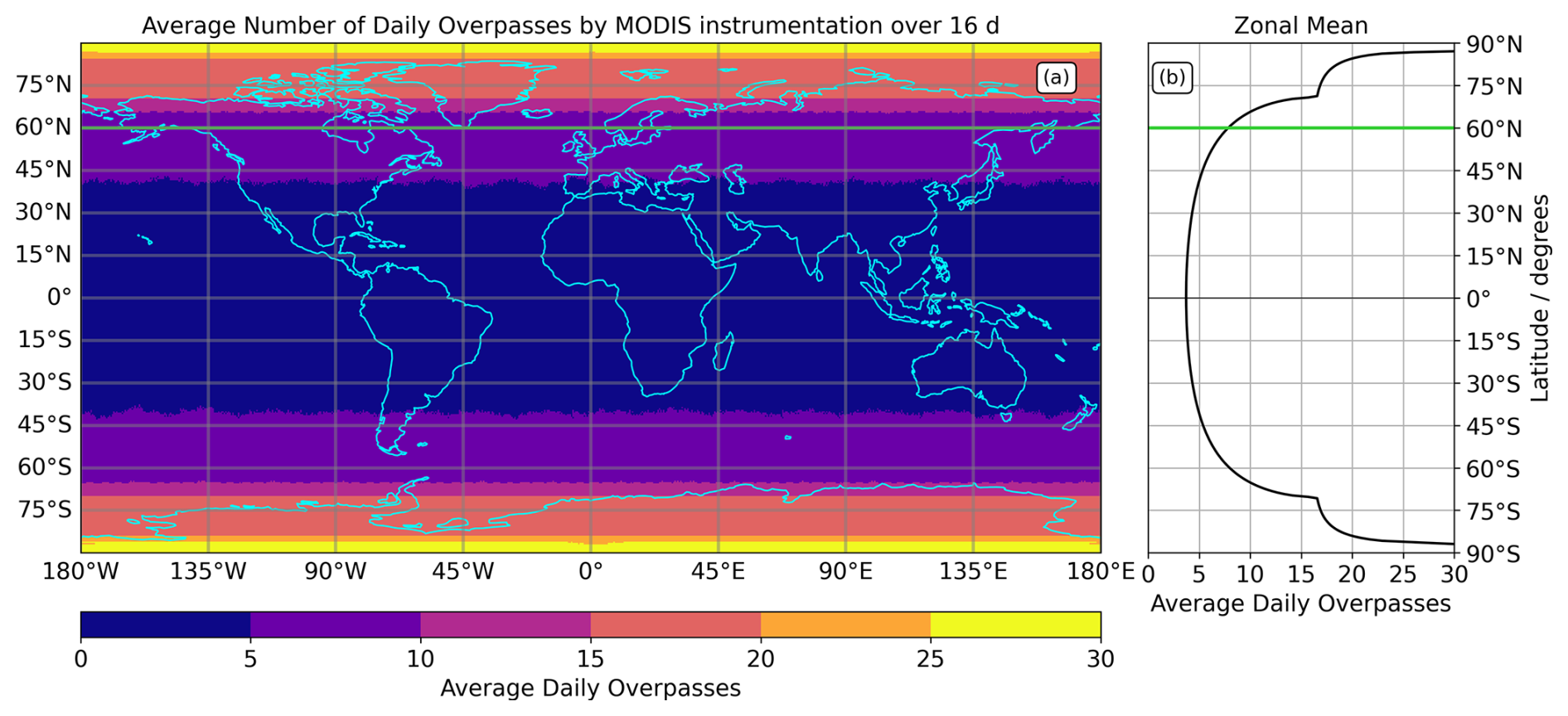
Figure 1 (a) Mean number of daily overpasses at any Earth location made by MODIS on AQUA and TERRA, and (b) zonal mean number of daily overpasses. Daily averages based on 16 d of data taken between 11 August 2024, 00:00 UTC and 27 August 2024, 00:00 UTC, gridded to a regular 0.5° × 0.5° grid. At latitudes where HL fires occur (60–75° N, green line and above), there is a latitudinal observation frequency dependence that provides on average between 8 and 18 daily satellite observations from these two systems alone. Each cloud-free observation provides an FRP measure, and which can be used to estimate FRE via temporal integration.

Given that geostationary observations of FRP are unsuitable for fire-prone HL regions, we aim to take advantage of the higher latitude, higher temporal resolution sampling of FRP of polar orbiting FRP observations to develop a HL version of the current FREM approach of Nguyen et al. (2023); generating a dataset of HL fire carbon and trace gas emissions completely independent of satellite-derived burned area measures and/or of the FRP-to-fuel consumption conversion coefficients influenced by them. These conversion coefficients are also not derived from small-scale experiments, but from Earth observation data of the landscape fires themselves. We compare our fire emissions assessments to those of existing state-of-the-art burned area and FRP based approaches, and assess the characteristics and benefits of our approach with respect to these alternatives. In Sect. 2, we provide the background to the FREM approach. In Sect. 3, we describe its adaptation for HL fires (hereby referring to the method as HLFREM) and using satellite derived polar orbiter FRP data and plume-integrated Total Column Carbon Monoxide (TCCO) observations we derive biome (“b”) specific emission coefficients for Carbon Monoxide (${\mathrm{EC}}_{\mathrm{CO}}^{\mathrm{b}}$) and Carbon (${\mathrm{EC}}_{\mathrm{C}}^{\mathrm{b}}$), as well as total CO and carbon emissions via their use with FRP time-series data. In Sect. 4, we calculate the total CO and Carbon emissions, using ${\mathrm{EC}}_{\mathrm{CO}}^{\mathrm{b}}$ and ${\mathrm{EC}}_{\mathrm{C}}^{\mathrm{b}}$, and compare them to the fire emissions estimates present in other widely used inventories, before closing with a Summary and Conclusion in Sect. 5.

2 FREM Background

As detailed in the review of Wooster et al. (2021), both geostationary satellites (Wooster et al., 2015; Xu et al., 2010, 2017, 2021) and polar-orbiting satellites (Giglio et al., 2016; Schroeder et al., 2014; Wooster et al., 2012; Xu et al., 2020) offer the capability to observe and quantify wildfire activity using Active Fire (AF) approaches involving FRP retrievals. Well-known inventories using these methods include the Fire Inventory from NCAR (FINN, Wiedinmyer et al., 2011), the Fire Energetic and Emission Research (FEER) approach (Ichoku and Ellison, 2014), the Quick Emission Dataset (QFED, Darmenov and da Silva, 2015), and GFAS (Kaiser et al., 2012). The most recently developed FREM method (Nguyen et al., 2023) directly links satellite-derived FRP data to a fires CO emission rate via a set ${\mathrm{EC}}_{\mathrm{CO}}^{\mathrm{b}}$ derived from a “matchup fire” subset of satellite-derived FRP and CO observations. Specifically, estimates of ${\mathrm{EC}}_{\mathrm{CO}}^{\mathrm{b}}$ are calculated using FRE and plume-integrated Total Column Carbon Monoxide (TCCO) data collected at a subset of “matchup fires” where both datasets are “well-observed” (e.g. no gaps in the FRP record, and a clear fire emissions CO plume is seen). Once derived, application of ${\mathrm{EC}}_{\mathrm{CO}}^{\mathrm{b}}$ to the FRP observations at all the regions fires enables the regions fire-related CO emission rates to be calculated without the need for any other information (Reid et al., 2009). Hence the approach is extremely direct, and with the emissions coefficients derived from the same types of satellite FRP data that they will ultimately be applied to, and thus which are impacted by the same factors such as overstory impacts on FRP measures and minimum FRP detection limits (Nguyen and Wooster, 2020).

Each FREM iteration thus far has relied on geostationary FRP data, due to its frequent 10-to-30 min imaging frequency enabling easy derivation of FRE (Wooster et al., 2021). Rather than CO however, the first FREM (v1) iteration focused on deriving aerosol optical depth (AOD) related total particulate matter (TPM) emissions from FRP observations (Mota and Wooster, 2018)_,an approach then enhanced by Nguyen and Wooster (2020) and Fisher et al. (2020) through the use of improved AOD datasets. FREMv2 (Nguyen et al., 2023) replaced use of AOD data with trace gas column amounts of CO (from the S5P (Sentinel-5 Precursor) observations using the TROPOMI (TROPOspheric Monitoring Instrument) sensor), directly estimating fluxes of CO rather than TPM. CO is the second largest fire-emitted compound after CO₂ (Akagi et al., 2011) and CO emissions factors are significantly less variable than those of TPM (Andreae, 2019). This makes any subsequent estimation of total fuel consumption using the FREM approach more appropriately conducted using CO pathway rather than one based on TPM fire emissions data.

3 High Latitude FREM Adaptation

As mentioned in Sect. 2, previous FREM studies have utilised geostationary observations of FRP, due to its high temporal sampling resolution of 10–30 min. However, a disadvantage of using geostationary platforms for FRP analysis is that the geostationary pixel areas grow rapidly at locations very far from nadir (>40° view zenith angle, Nguyen and Wooster, 2020; Xu et al., 2021), thus making geostationary platforms unsuitable for HL FRP studies.

The polar-orbiting based HLFREM framework developed herein builds on the geostationary FREM methods by identifying a set of matchup fires for which both the total amount of CO contained in the fire plume is assessed, as well as the total amount of FRE released over the time it took the plume to form (Sect. 3.4). Using these polar-orbiting matchups, a set of ${\mathrm{EC}}_{\mathrm{CO}}^{\mathrm{b}}$ are generated using ordinary least squares (OLS) linear best fits to the co-incident FRE and CO data of all matchup fires in that biome. These ${\mathrm{EC}}_{\mathrm{CO}}^{\mathrm{b}}$ can then be multiplied by the regionally complete FRP time-series, including potentially hundreds of thousands more fires than are included in the matchup datasets, generating a spatially and temporally comprehensive set of biomass burning CO emissions covering all fires. Dividing these CO emissions by the standard biome-specific Emissions Factors (EFs, Akagi et al., 2011; Andreae, 2019) provides estimates of dry biomass consumption and also of total carbon (assuming biomass is 50±5 % carbon), or via use of EF ratios of any trace gas to CO also estimates of other trace gas emissions totals (Nguyen et al., 2023; Nguyen and Wooster, 2020).

A brief description of the data used for the HLFREM biome specific emission coefficient is shown in Sect. 3.1, with a description of the region of interest in Sect. 3.2. The full selection process for the fire matchups to which this procedure is applied is described in Sect. 3.3; and at each fire the relevant FRE was calculated as described in Sect. 3.4 using as the temporal integration period the time between the early morning fire activity minimum and the S-NPP VIIRS overpass made almost simultaneously to that of S5P (Sect. 3.5). Once sufficient matchup fires existed for each fire biome covered (see Sect. 3.6), we generated ${\mathrm{EC}}_{\mathrm{CO}}^{\mathrm{b}}$ for these biomes as detailed in Sect. 3.7. These emission coefficients were then multiplied by the full GFAS v1.2 FRP record (January 2003–December 2024, Sect. 4.1), to generate a HLFREM CO emission timeseries. Additionally, via the application of the appropriate EFs, it was also possible to generate a HLFREM Carbon emission timeseries using GFAS v1.2 (Sect. 4.2). For both the CO and Carbon emission timeseries, the HLFREM emissions will be compared to pre-existing emission databases; namely FEER, GFAS v1.2, and GFED v4.1s.

3.1 HLFREM Earth Observation Data Used

3.1.1 VIIRS and MODIS multispectral

Satellite observations from the Visible Infrared Imaging Radiometer Suite (VIIRS) onboard the Suomi National Polar-orbiting Partnership (SNPP) and the Moderate Resolution Imaging Spectroradiometer (MODIS) instruments onboard the Terra and Aqua platforms were used in order to manually identify matchup fire locations (Sect. 3.3).

The SNPP satellite was launched in 2011 and operates in a sun-synchronous orbit with equatorial crossing local times of approximately 01:30 and 13:30. The VIIRS instrument provides simultaneous, co-registered measurements at 375 and 750 m spatial resolution across 22 spectral bands spanning the visible to longwave infrared spectrum. These observations support the generation of a wide range of operational environmental products. In this study, fire detections were obtained from the VIIRS active fire product (VNP14, Schroeder et al., 2014), while aerosol loading was characterised using Aerosol Optical Depth (AOD) retrievals produced by the Enterprise Processing System (AOD EPS, NOAA, 2020).

The MODIS instruments onboard Terra and Aqua provide a longer observational record, with launches in 1999 and 2002, respectively. Both instruments operate in sun-synchronous orbits, with initial equatorial crossing local times of 10:30/22:30 for Terra and 01:30/13:30 for Aqua. However, gradual orbital drift has resulted in changes to these nominal observation times over the course of the missions. MODIS provides simultaneous, co-registered observations at 250, 500, and 1000 m spatial resolutions across 36 spectral bands covering the visible through longwave infrared wavelengths. Like with the VIIRS observations, The MODIS active fire products (MOD14 and MYD14, Giglio et al., 2016) were also used for matchup fire identification.

3.1.2 TROPOMI TCCO

The TROPOMI sensor onboard the European Space Agency (ESA) S5P satellite orbits the globe with an equatorial ascending and descending node of approximately 13:30 and 01:30 respectively; very similar to that of the Visible Infrared Radiometer Suite (VIIRS) onboard Soumi National Polar-orbiting Partnership (S-NPP, Jing et al., 2022). Onboard TROPOMI are four spectrometers, covering the ultraviolet-visible, near infrared, and shortwave infrared (SWIR) spectral bands (Veefkind et al., 2012). Amongst other species, such as NO₂, CH₄, and O₃, TCCO is observed, at a spatial resolution of approximately 5.5×7.0 km (August 2019 to present, 7.0×7.0 km prior to August 2019, Inness et al., 2022), derived using SWIR observations with the Shortwave Infrared CO Retrieval (SICOR, Landgraf et al., 2016) algorithm. The TROPOMI TCCO observations have been validated against both ground-based remote sensing techniques (such as the Total Carbon Column Observating Network, TCCON, Borsdorff et al., 2018) and through space-based remote sensing techniques (Martínez-Alonso et al., 2020; Neyra-Nazarrett et al., 2025).

The S5P TCCO product includes a quality flag, indicating the potential presence of cloud in the resulting TCCO pixel. For this study, we have used observations with a quality flag of ≥0.5, aligning with the recommended quality threshold (Apituley et al., 2018) and other TCCO studies (Griffin et al., 2024; Nguyen et al., 2023; Rowe et al., 2022). The impact of using only pixels with a quality flag of >0.5 was small, given that the quality flags in the TCCO product were carried out in clear-sky only conditions; a requirement of the FREMv2 methodology (Borsdorff et al., 2018; Nguyen et al., 2023).

3.1.3 Global Fire Assimilation System (GFAS) FRP

The regionally comprehensive FRP time-series used herein, replacing the geostationary FRP time-series used in FREMv2, is the Global Fire Assimilation System (GFAS v1.2) FRP dataset described in Kaiser et al. (2012), generated as part of the Copernicus Atmospheric Monitoring Service (CAMS: https://atmosphere.copernicus.eu/, last access: 2 September 2026) and widely used (e.g. Di Giuseppe et al., 2018; Inness et al., 2019; Popovicheva et al., 2022) The GFAS v1.2 record is based on per-pixel FRP retrievals contained within the Terra/Aqua MOD14/MDY14 active fire products (Giglio et al., 2016), using these to generate daily mean cloud-adjusted FRP data gridded at 0.1° back to almost the start of the MODIS mission (Kaiser et al., 2012). At the high latitudes, the GFAS FRP record will include more FRP observations from the polar-orbiting MODIS platform, due to orbital convergence (Fig. 1).

However, whilst the GFAS v1.2 FRP data dating back to 2003 are considered a suitably long FRP time-series for generating a long-term CO emissions record, they are less well suited to the initial generation of the ${\mathrm{EC}}_{\mathrm{CO}}^{\mathrm{b}}$ coefficients linking FRP to rate of CO emissions since they provide only daily average FRP values. Specifically, the daily average FRP data contained in GFAS v1.2 cannot be used to estimate the amount of FRE emitted by a fire from the night-time FRP minimum up until the early afternoon TROPOMI overpass, since only daily average FRP is provided, and yet this sub-daily FRE value is required at the set of matchup fires to generate the initial ${\mathrm{EC}}_{\mathrm{CO}}^{\mathrm{b}}$ emissions coefficients. For this reason, these coefficients were instead derived using the alternative GFAS v1.4 implementation (Kaiser et al., 2024), which applies the fire diurnal cycle model of (Andela et al., 2015) to the 0.1° gridded MODIS FRP used to generate GFAS v1.2 but now to obtain hourly gridded FRP estimates. A comparison of a GFASv1.2 and GFASv1.4 global FRE estimates for 2020 showed that they were in good agreement with each other (Fig. 2), with a coefficient of determination (r²) of 0.908, and a mean bias of 0.13 PJ, indicating negligible systematic differences between the two datasets, and an RMSE of 3.53 PJ and a standard deviation of 3.53 PJ, reflecting variability in the FRE estimates between the two datasets, due to the inclusion of a diurnal FRP model into GFASv1.4.

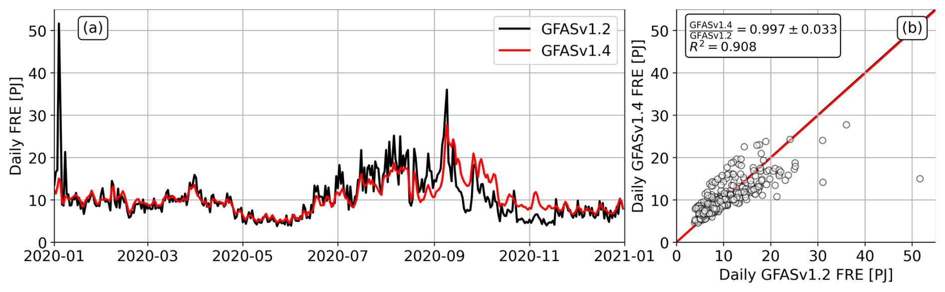
Figure 2 (a) Daily global FRE estimated from GFASv1.2 (black) and GFASv1.4 (red) throughout 2020. (b) Scatter of Daily global FRE estimates from GFASv1.2 and GFASv1.4.

At the location of each matchup fire, these hourly FRP data can then be integrated over the required time period from the night-time fire minimum up until the S5P (TROPOMI) satellite overpass time to generate the FRE released. Though GFAS v1.4 goes back only to 2019, this is perfectly sufficient for deriving the ${\mathrm{EC}}_{\mathrm{CO}}^{\mathrm{b}}$ coefficients.

3.2 Region of Interest Selection

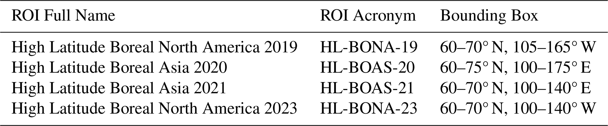
HL fire is seasonal in nature, dominantly present in the Northern Hemispheric Summer months (June, July, August, Fig. 3a). Four HL ROIs and matching time periods were used from within this period to generate the set of matchup fire, and each of the ROI extractions focused on a period when fire activity was maximised in that ROI, as shown in Fig. 3b and c, and detailed in Table 1. Landcover data, natively at 300 m grid resolution, taken from the ESA Climate Change Initiative (ESA-CCI) 2018 land cover map (ESA, 2017) was used to classify biomes within the ROI's, based on 11 “fire-biome” classes aggregated from the original 37 landcovers (Table A1 in Appendix A), as shown in Fig. 3b. The two ROIs in Boreal Asia (HL-BOAS-20 and HL-BOAS-21) were dominated by the Deciduous Needleleaf Forest fire biome, whereas those in Boreal North America (HL-BONA-19 and HL-BONA-23) were dominated by Evergreen Needleleaf Forest fire biome.

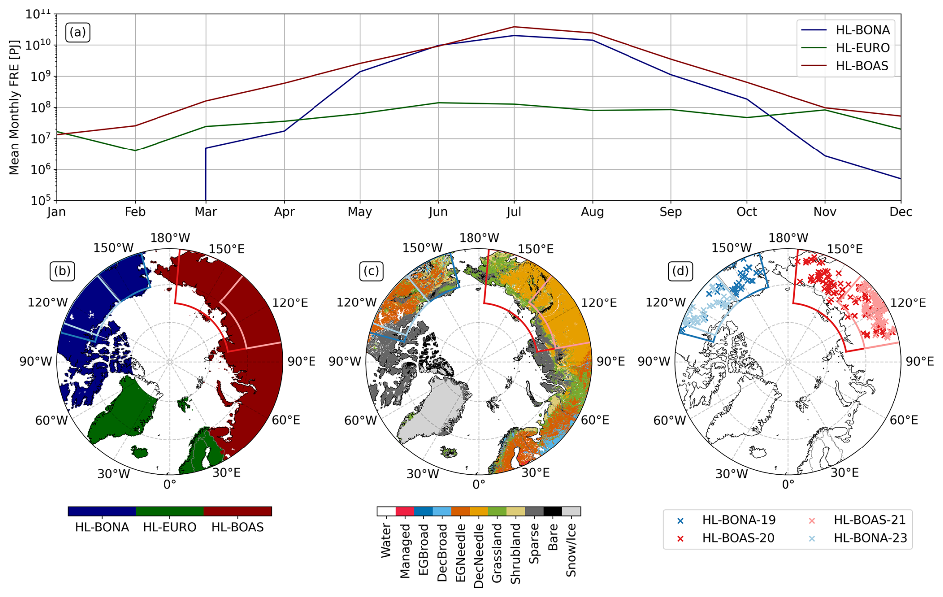
Figure 3 HL fire information. (a) Mean monthly FRE (2003–2024) for HL fires (≥60° N) in the regions used by the Global Fire Emissions Database (GFED; Randerson et al., 2017, BONA: Boreal North America, EURO: Europe, BOAS: Boreal Asia), as derived from GFAS v1.2. (b) HL regions used for the mean monthly FRE estimation in (a), as defined by GFED. (c) ROI and aggregated fire biome map, as derived from the CCI Land Cover 2018 map (ESA, 2017) and with biome aggregation detailed in Table A1. (d) The four ROIs used in this study within which the 833 fire-matchup (shown as crosses) were identified. GFAS v1.2 data courtesy of Copernicus Atmosphere Monitoring Service (CAMS)/ECMWF. CCI Land Cover 2018 data courtesy of ESA/Copernicus Climate Change Initiative.

Table 1 Acronyms and Geographic bounding boxes of ROIs, as shown in Fig. 3c.

3.3 Plume Identification

Within each of the four ROIs shown in Fig. 2b and c, the potential cloud-free matchup fires were manually identified and examined via visual inspection of multispectral and AF Products detailed in Table 2, based on the following criteria:

• Clear smoke emission visible in the VIIRS true colour (Red: M05, Green: M04, Blue: M03) imagery, and without apparent mixing with other nearby smoke plumes.

• Clear visual indication of a developed smoke plume, spread by the wind, in the same VIIRS true colour imagery.

• Clear identification of a region of shortwave infrared thermal emission (hereby referred to as the “burning area”) resulting from active combustion, as seen in a VIIRS false colour (Red: M11, Green: I02, Blue: I01) imagery.

• AF Pixels present within the “burning area” as deduced from the VIIRS VNP14 and MODIS MOD14/MYD14 AF Products.

Table 2 Satellite data products used during the manual inspection and digitization of matchup fire polygons.

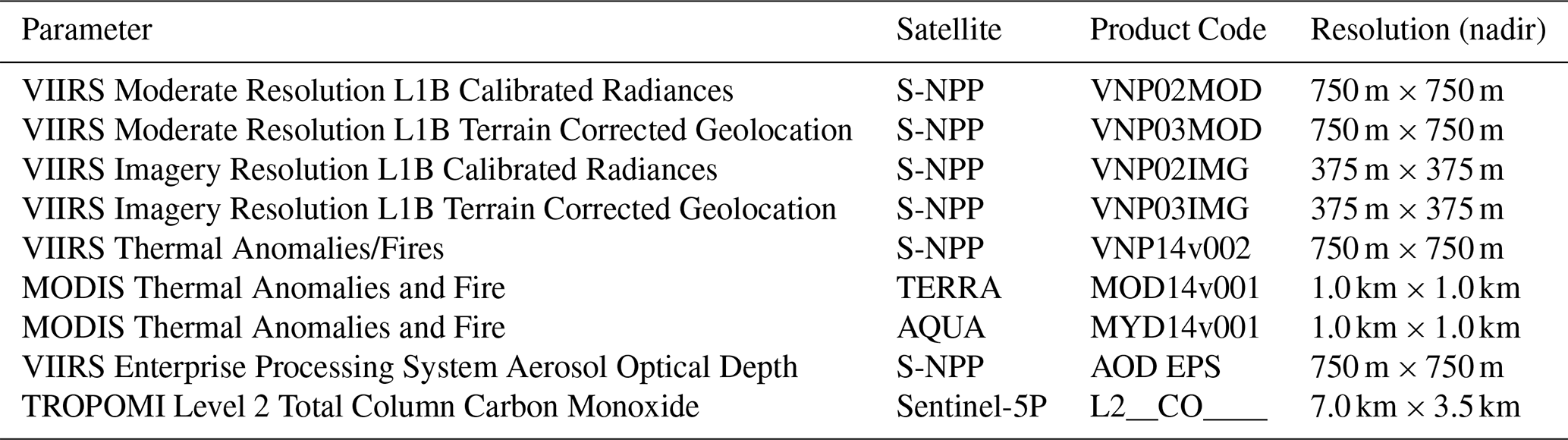
Each potential matchup fire then had its smoke plume and associated burning area extent digitized and examined; based on manual interpretation of the VIIRS multispectral imagery, matching VIIRS AF and Aerosol optical depth (AOD) products (NOAA, 2020), and TROPOMI TCCO products, as shown in Fig. 4.

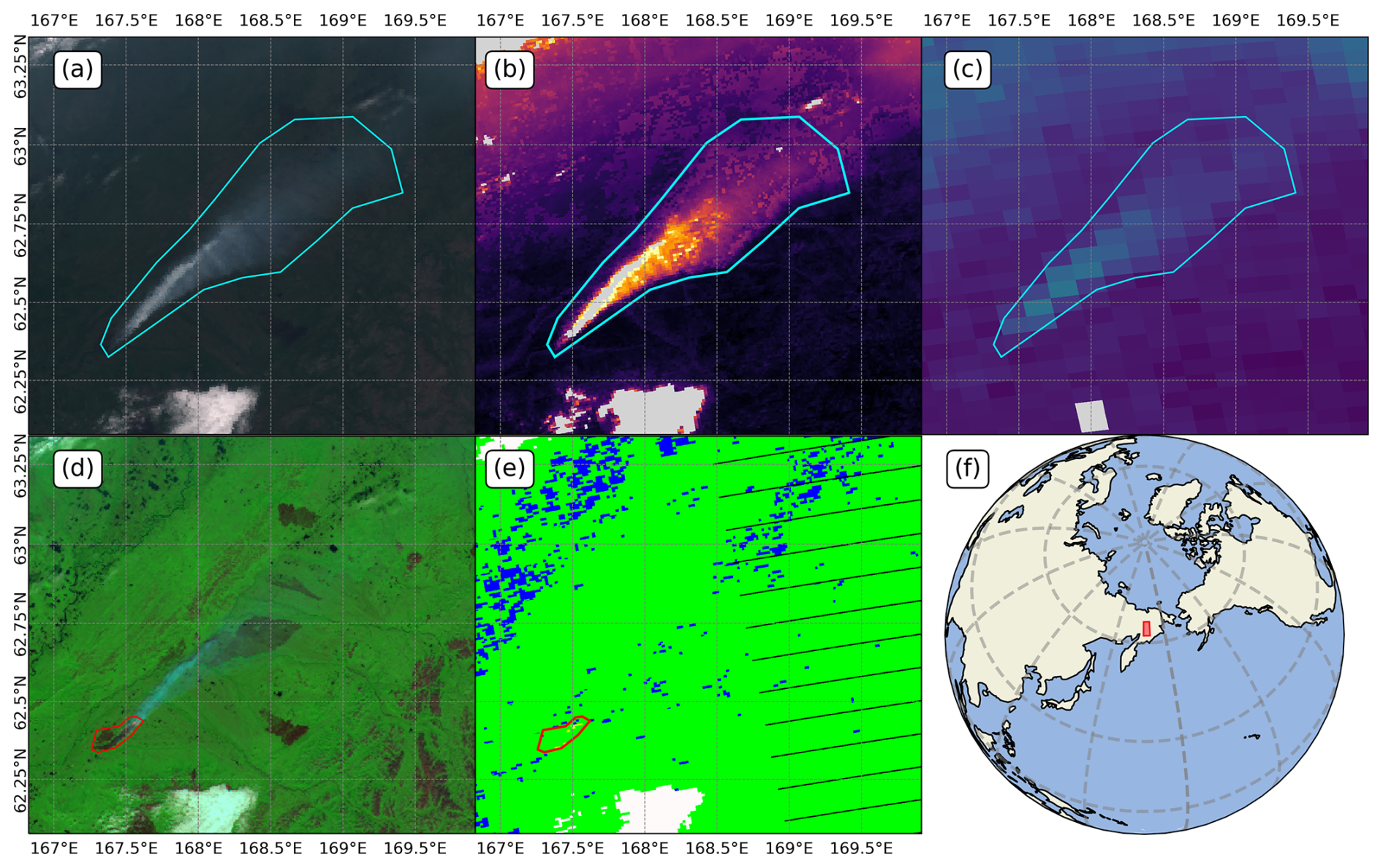
Figure 4 Example of a matchup fire imaged in Siberia (62.39° N, 167.49° E) on 28 July 2020 at 01:42 UTC (13:42 PETT). The digitised outline of the plume (cyan) and burning area (red) are shown superimposed on (a) RGB (M05-M04-M03) imagery via S-NPP (VIIRS), (b) AOD (processed via EPS) from S-NPP (VIIRS), (c) Sentinel-5P TCCO data, (d) False Colour Composites (M11-I02-I01) via S-NPP (VIIRS), (e) VIIRS Active Fire Product (VNP14) from S-NPP (VIIRS). Green: Non burning vegetation. Yellow: Active Fire Hotspot, Blue: Water, White: Cloud, Black: No Data. (f) Geographic location and extent of the plots shown (red). VIIRS imagery courtesy of NOAA/NASA (S-NPP). AOD processing courtesy of EUMETSAT EPS. Sentinel-5P TROPOMI data courtesy of ESA/Copernicus. VIIRS Active Fire Product (VNP14) courtesy of NASA/NOAA.

3.4 Fire Radiative Energy Estimation

To calculate the FRE for each matchup fire, each digitised burning area polygon was converted to a binary mask and used to extract the FRP time-series from the hourly-timestep FRP record held within GFAS v1.4 (see example in Fig. 5) for all GFAS v1.4 pixels that intersect with or are contained by the burning area polygon. HL orbital convergence ensured the calculation was based on significantly more polar-orbiting observations than would be the case at lower latitudes (Fig. 1), and, following (Nguyen et al., 2023), the FRP integration took place from the 06:00 local time fire activity minima (Fig. A1 in Appendix A) up until the time of the almost simultaneous early afternoon S5P and Suomi S-NPP overpasses. Mean FRP record length for all matchup fires was 7.3 h (minimum 4 and maximum 11 h), with the variation due to the orbital convergence (Fig. 1) and this results in the match-up fires being observed by Sentinel-5P up to three times per day from different ascending overpasses.

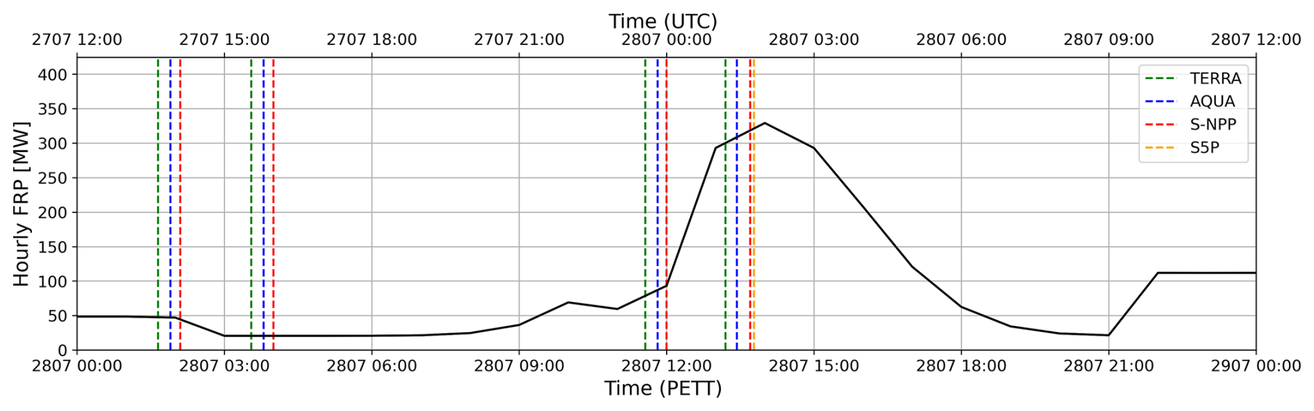
Figure 5 Example of the hourly FRP time-series from GFAS v1.4, used to generate an FRE measure for a single matchup fire (i.e. the match-up fire in Fig. 4, as shown above). The hourly FRP timeseries data were generated from the set of individual FRP observations provided by MODIS on AQUA and TERRA, using the diurnal cycle model of Andela et al. (2015). Additionally, the VIIRS observations on S-NPP used for fire-matchup identification are also shown. Times of the individual satellite overpasses, as well as of the S5P overpass time used to provide the TCCO data for this fire-matchup, are indicated.

3.5 Excess CO Estimation

For each fire-matchup, the smoke plume polygon with a surrounding buffer of one pixel was also used to generate a binary mask employed to extract the relevant S5P TROPOMI TCCO data within the plume for a given S5P overpass, along with a measure of the ambient background TCCO (TCCO_BG, taken as the minimum TCCO within the buffered mask). Total excess plume CO (CO_EX) was then calculated for each fire-matchup, as the sum of all CO_EX from each S5P pixel associated with each fire-matchup, using Eq. (1).

$$\begin{array}{}\text{(1)}& {\mathrm{CO}}_{\mathrm{Ex}}=\sum \left({\mathrm{TCCO}}_{\mathrm{M}}-{\mathrm{TCCO}}_{\mathrm{BG}}\right)\cdot A\cdot M_{\mathrm{CO}}\end{array}$$

where TCCO_M is the TCCO within the buffered binary mask (units: mol m⁻²), TCCO_BG is the ambient background TCCO (units: mol m⁻²), A is the S5P pixel size (units: m²) calculated from the geographic coordinates of the pixel corners, and M_CO the molecular weight of CO (units: g mol⁻¹). Due to orbital convergence, a single fire can be observed multiple times by Sentinel-5P. Each individual overpass is treated as an independent observation. As a result, a single landscape fire event may correspond to multiple matchup fire events within the matchup dataset, each associated with a different estimate of excess CO (due to overpasses occurring approximately 100 min apart).

3.6 Fire Biome Estimation

All MODIS and S-NPP AF pixels within the fires burning area polygon and timed during the FRP temporal integration period had their fire-biome determined using the aggregated biome data shown in Fig. 3b. For a single fire if ≥ 50 % of the AF pixels were from a single fire-biome then that was set as the fires “dominant” fire-biome. Fires having no such dominant class were discarded, as their derived emission coefficients could not be properly allocated to a fire-biome.

3.7 Biome Specific Emission Coefficient Generation

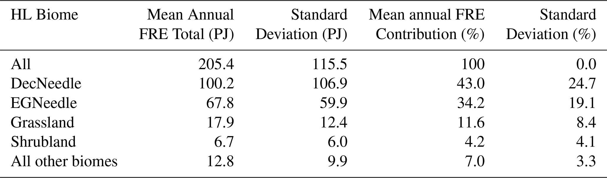
In total, 833 individual matchup fires were initially identified across the four regions of interest (Table 1), in their respective Northern Hemispheric months, with 125 of those being discarded as having no dominant fire-biome. Of the 708 fires remaining, 468 were located in Deciduous Needleleaf Forest (DecNeedle), 186 in Evergreen Needleleaf Forests (EGNeedle), 26 in Grassland, 22 in Shrubland, and six in a fire-biome described as “Sparse”. The locations of the matchup fires for the four most well-sampled fire-biomes identified (DecNeedle, EGNeedle, Grassland, and Shrubland) are mapped in Fig. 3c. Analysis of the mean annual FRE totals from GFAS v1.2 (Fig. 6, Table 3) shows that these four biomes are responsible for the vast majority (∼93 %) of the total FRE generated by HL fires.

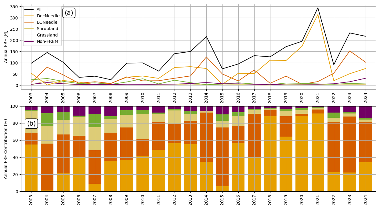
Figure 6 Mean annual HL FRE (a) totals (PJ), and (b) contribution (%) of each of the four most well sampled biomes identified as part of the fire-matchups database, as well as from additional biomes, taken from GFAS v1.2 (2003–2024).

Table 3 Mean Annual FRE totals (PJ) and contribution (%) for each of the four most well sampled biomes, compared to all other HL biomes, calculated using GFAS v1.2, between 2003 and 2024.

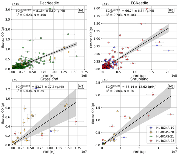
Following Nguyen et al. (2023), the FRE and Excess CO data of each fire-biomes matchup fires were used to derive a set of ${\mathrm{EC}}_{\mathrm{CO}}^{\mathrm{b}}$ emissions coefficients via zero-intercept OLS linear regression (Fig. 7); with results reported in Table 4. As detailed in Nguyen and Wooster (2020), “FEER-equivalent” ${\mathrm{EC}}_{\mathrm{CO}}^{\mathrm{b}}$ values are also reported therein, calculated from the grid cell (not biome) based FRE-based total particulate matter (TPM) emissions coefficients (${\mathrm{EC}}_{\mathrm{TPM}}^{\mathrm{b}}$) reported in Ichoku and Ellison, (2014) (available at https://feer.gsfc.nasa.gov/data/emissions/, last access: 19 March 2025) and the relevant biomes TPM-to-CO EF ratios (Nguyen and Wooster, 2020). The HLFREM ${\mathrm{EC}}_{\mathrm{CO}}^{\mathrm{b}}$ values reported in Fig. 7 and Table 4 are similar in magnitude to the emission coefficients reported in Griffin et al. (2024), who developed global emission coefficients using a mass balance approach to determine a relationship between TROPOMI observations of CO and MODIS observations of FRP, according to different biome classifications. Whilst the GFEDv4 biome classification is not limited to HL regions only, the similarity in the forested HLFREM ${\mathrm{EC}}_{\mathrm{CO}}^{\mathrm{b}}$ values to the Griffin et al. (2024) BORF ${\mathrm{EC}}_{\mathrm{CO}}^{\mathrm{b}}$ is encouraging.

Table 4 Emissions coefficients for CO (${\mathrm{EC}}_{\mathrm{CO}}^{\mathrm{b}}$) as derived in Fig. 7, along with FEER-equivalent values for comparison and those for carbon (${\mathrm{EC}}_{\mathrm{C}}^{\mathrm{b}}$) calculated using ${\mathrm{EC}}_{\mathrm{CO}}^{\mathrm{b}}$ and EFs from Andreae and Merlet (2001) and Akagi et al. (2011) – labelled -AM, and -AG respectively, in Sect. 4.2. Also shown are ${\mathrm{EC}}_{\mathrm{CO}}^{\mathrm{b}}$ for GFEDv4 biomes (in brackets), as derived by Griffin et al. (2024).

Analysis comparing the spatial distribution of FRP across the entire Northern Hemispheric Summer (JJA) HL GFASv1.4 dataset with those relating to the matchup fires can be found in Fig. 8. It can be seen that the matchup fires are spatially well sampled across the JJA GFASv1.4 dataset (Fig. 8a, b, and d), with matchup fires being found across the fire-prone HL-BONA region, and the eastern half of the fire-prone HL-BOAS region (≥100° E). Additionally, it can be seen the matchup fires tended to be comprised of a greater proportion of higher FRP observations (Fig. 8e), which did not have a zonal or a longitudinal bias in them, as the zonal and longitudinal mean FRP of the matchup fires were consistently higher than those of the JJA GFASv1.4 dataset (Fig. 8c and e). A Mann-Whitney U test was performed on the matchup fire FRP values (containing n=73 951 pixels, median FRP: 76.5 MW) and remaining JJA GFASv1.4 FRP values (containing = 4 414 203 pixels, median FRP: 11.4 MW), showing that the distributions differed significantly ($U=\mathrm{7.92}\times {\mathrm{10}}^{\mathrm{10}}$, p<0.001, rank-biserial correlation = 0.515), indicating preferable sampling of higher FRP values. This is to be expected, as the plume identification criteria (Sect. 3.3) requires a clear visual indication of a developed smoke plume with an associated area of active combustion; the likelihood of which increases with increasing FRP, when occurring under the same conditions. Smaller fires are likely not going to produce an optically visible smoke plume, and are thus unlikely to result in selection for digitization. Fires that occur underneath pre-existing smoke plumes are also not going to be picked for plume digitization, as the CO enhancement could not be accredited to an individual smoke plume.

An OLS regression was selected because the uncertainties associated with the excess CO and FRE estimates for a given matchup fire data point included potentially unmeasured sources of variability. Although both variables contain measurement and retrieval uncertainties (Griffin et al., 2024; Rowe et al., 2022), these uncertainties do not represent all sources of variability affecting the relationship between excess CO and fire activity, with some contributions of uncertainty being unquantifiable (Nguyen et al., 2023). Due to this, a regression method that is driven by data point uncertainty (such as orthogonal distance regression) was deemed unsuitable for use.

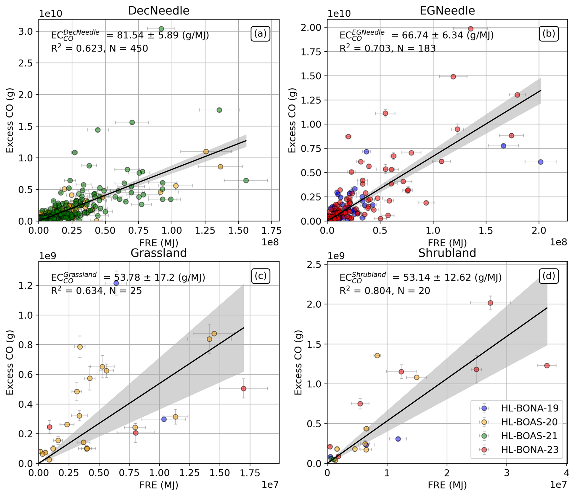
Figure 7 HLFREM biome-specific CO emission coefficients (${\mathrm{EC}}_{\mathrm{CO}}^{\mathrm{b}}$, in g MJ⁻¹) derived from the set of matchup fires for (a) Deciduous Needleleaf Forests, (b) Evergreen Needleleaf Forests, (c) Grasslands, and (d) Shrubland fire-biomes. Each datapoint represents a single matchup fire that had its plume total Excess CO and total released FRE assessed for a matching time-period, and the ${\mathrm{EC}}_{\mathrm{CO}}^{\mathrm{b}}$ value for the fire-biome is derived from the slope of the OLS linear best fit (solid black line) to these data. Colour of the scatter points denotes the ROI containing the fire (see Fig. 3c). Error bars denote the standard deviation of FRP values and the uncertainty in the S5P TCCO produce respectively, as calculated following (Nguyen et al., 2023). The shaded area indicates the uncertainty on the slope of the linear best fit, taken to be the uncertainty on the derived ${\mathrm{EC}}_{\mathrm{CO}}^{\mathrm{b}}$ value.

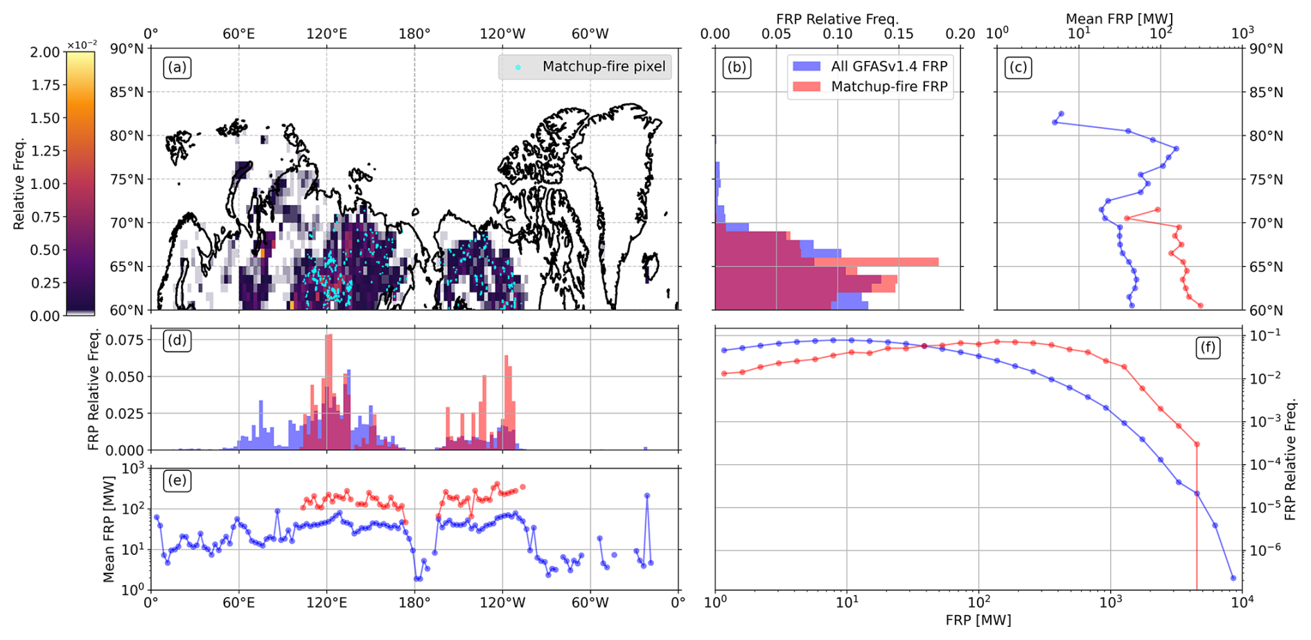
Figure 8 Spatial analysis comparison of GFASv1.4 FRP values (2019–2024, JJA) and matchup fires selected from GFASv1.4. (a) Relative frequency of FRP observations plotted against matchup-fire pixel locations. (b) Zonal FRP relative frequency (1° bins) for All GFASv1.4 (JJA) pixels and matchup-fire pixels. (c) Zonal mean FRP value frequency (1° bins) for all GFASv1.4 (JJA) pixels and matchup-fire pixels. (d) Longitudinal FRP relative frequency (2.5° bins) for all GFASv1.4 (JJA) pixels and matchup-fire pixels. (e) Longitudinal mean FRP (2.5° bins) for all GFASv1.4 (JJA) pixels and matchup-fire pixels. (f) FRP relative frequency for all GFASv1.4 (JJA) pixels and matchup-fire pixels.

It should be noted that the emission coefficients shown in Fig. 7, as well as the matchup fire dataset they are derived, assume a single relationship between CO emissions and FRE for a given biome. In reality, this is unlikely to be the case, as combustion phase and the relative contributions of flaming and smouldering combustion can heavily influence the fire behaviour, and resulting smoke and emission characteristics (Freeborn et al., 2008; Reid et al., 2009). However, no current space-based EO approach for estimating landscape fire emissions explicitly accounts for variability in combustion phase (Owsley-Brown et al., 2024). Additionally, satellite-derived FRP represents an instantaneous measurement of radiative power and provides no direct information on the relative proportions of flaming and smouldering combustion occurring within the observed fire.

The uncertainty bars associated with the emission coefficients in Fig. 7 account for two primary sources of uncertainty. Firstly, the estimated uncertainty in the Sentinel-5P CO retrievals, including the approximate 10 % bias relative to TCCON observations (Sha et al., 2021). Secondly, the spatial variability of both the excess CO estimations and the FRP within each fire polygon, represented by their standard deviations. In addition to these quantified sources of uncertainty, the spread of the individual matchup fires contributing to each biome-specific emission coefficient is also likely to reflect natural variability in the combustion phases, particularly differences in the proportion of flaming and smouldering activity between fires.

Additionally, the emission coefficients shown in Fig. 7, together with the matchup fire dataset they are derived from, do not explicitly account for peat or organic soil combustion, and therefore do not distinguish between regions of high or negligible organic soil content, which may lead to an underestimation of CO emission from fires within peat-rich environment. Organic soil content was considered as a potential additional classification variable during the matchup fire dataset creation, via use of the global PEATMAP product (Xu et al., 2018). However, incorporating this information reduced the sample sizes of each individual classification, limiting the reliability of the respected OLS regressions. Therefore, as with the combustion phase, the emission coefficients implicitly assumes a uniform contribution of organic soil combustion across the entire matchup fire dataset. This assumption, like that with combustion phase, likely contributes the variability of the individual matchup fires within Fig. 7, which is reflected in the uncertainty of the fitted OLS regressions.

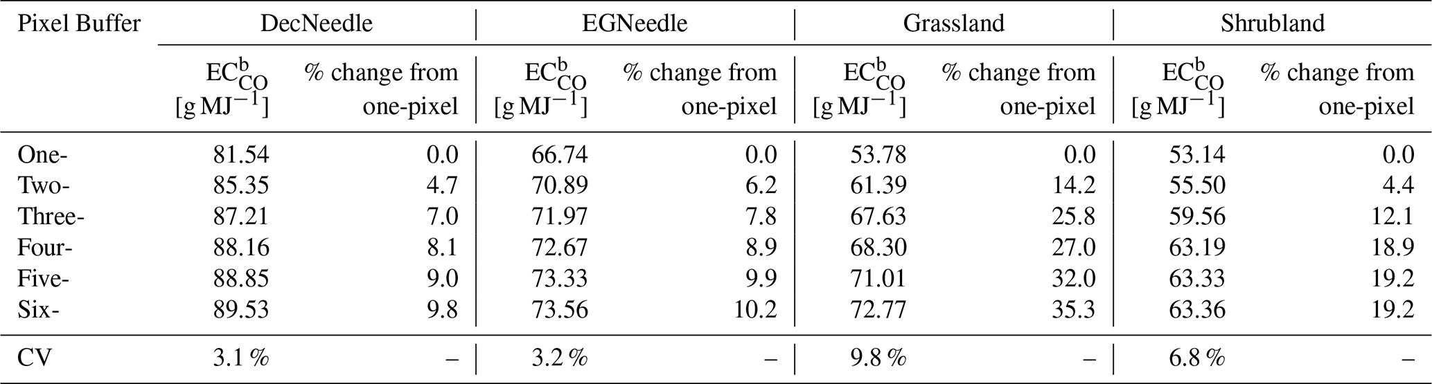
In order to assess the impact of using the one-pixel buffer around the digitized plume polygon, the excess CO calculation was repeated, using an increasing number of pixels as the buffer (specifically, a one-, two-, three-, four-, five-, and six-pixel buffer) to capture TCCO_BG. ${\mathrm{EC}}_{\mathrm{CO}}^{\mathrm{b}}$ were recalculated, using the new excess CO values from the corresponding pixel buffer (Fig. A2 in Appendix A). Table 5 details the calculated ${\mathrm{EC}}_{\mathrm{CO}}^{\mathrm{b}}$ for each biome and pixel buffer, along with the percentage change from the one-pixel buffer. It can be seen that for the forested (DecNeedle and EGNeedle) and shrubland biomes, the ${\mathrm{EC}}_{\mathrm{CO}}^{\mathrm{b}}$ increased with increasing pixel buffer, before approaching a plateau between three and four pixels. Beyond this point, further expansion of the buffer resulted in relatively small increases in ${\mathrm{EC}}_{\mathrm{CO}}^{\mathrm{b}}$ (<3 % for both forested biomes, and <1 % for shrubland biomes), suggesting that most of the excess CO associated with the plume had already been captured. In contrast, the grassland ${\mathrm{EC}}_{\mathrm{CO}}^{\mathrm{b}}$ exhibited a stronger dependence on plume buffer size, increasing approximately 35 % between the one- and five-pixel buffers, indicating greater sensitivity to plume buffer size. However, the one-pixel buffer was adopted for all subsequent analyses, to maintain methodological consistency with previous FREMv2 studies. The sensitivity analysis demonstrated that this choice introduces relatively small differences for the forest and shrubland biomes (Coefficient of variation, CV = 3.1 %–6.8 %), although a larger sensitivity was observed for grassland (CV = 9.8 %).

Table 5 ${\mathrm{EC}}_{\mathrm{CO}}^{\mathrm{b}}$ values calculated using one- to six-pixel buffers to estimate TCCO_BG. Scatterplots from which ${\mathrm{EC}}_{\mathrm{CO}}^{\mathrm{b}}$ was calculated can be found in Figs. 7 (for one-pixel buffer) and A2 (for two- to six-pixel buffer).

4 Emission Inventory Comparisons

4.1 High Latitude Carbon Monoxide Emission Timeseries

To generate a long-term CO emissions timeseries for the HL biomes, we applied the derived ${\mathrm{EC}}_{\mathrm{CO}}^{\mathrm{b}}$ emissions coefficients to the GFAS v1.2 FRP data available from the current time back to almost the start of the MODIS record (2003). The resulting monthly and annual CO emissions timeseries are shown in Fig. 9. Also shown are the FEER-equivalent CO timeseries, the CO emissions that come as part of the GFAS v1.2 dataset derived from the FRP values as per Kaiser et al. (2012), and the GFED v4.1s CO emissions (2003–2024). The mean annual CO emissions for the four biomes using HLFREM, FEER, GFAS v1.2, and GFED v4.1 can be found in Table 6, and note that of these four datasets, the same MODIS FRP data drive the emissions estimates in HLFREM, GFAS v1.2 and FEER, whilst GFED v4.1s uses primarily MODIS burned area data (Giglio et al., 2013). However, also note that the conversion coefficients linking daily mean FRP to biomass burned in GFAS v1.2 as a prior step to its CO emissions estimation were generated using linear regression against burned biomass estimates of an earlier version of GFED (Kaiser et al., 2012). HLFREM removes this link by directly relating the daily FRE measures to CO fluxes via the conversion coefficients derived from FRP and Sentinel-5P CO data at the matchup fires.

Table 6 Mean annual (2003–2024) CO emissions for the inventory-biome pairs. Uncertainty values are the standard error of the mean.

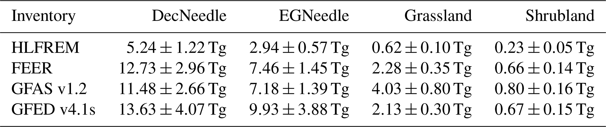
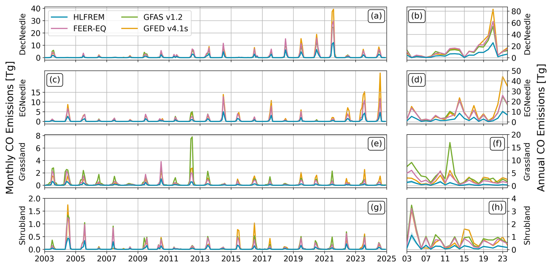
Figure 9 Timeseries of Monthly (a, c, e, g) and Annual (b, d, f, h) HL Wildfire emissions of CO for (a, b) DecNeedle, (c, d) EGNeedle, (e, f) Grassland, and (g, h) Shrubland biomes, calculated using the ${\mathrm{EC}}_{\mathrm{CO}}^{\mathrm{b}}$ from HLFREM (blue) and FEER (red) as detailed in Table 4 using daily FRE totals generated by GFAS v1.2. GFAS v1.2 (green) and GFED v4.1s (orange) CO emissions for the same biomes are shown in green. OLS regression analysis can be found in Fig. A3 in Appendix A.

It can be seen from Fig. 8 that the temporal patterns of HLFREM CO emissions across all biomes are consistent with those from the other three inventories, with the temporal patterns being more pronounced in the two forested and Shrubland biomes. This is to be expected with respect to GFAS v1.2 and FEER-EQ, as HLFREM, GFAS, and FEER-EQ emissions all use the same FRP input (GFAS v1.2). The peaks also match independent reports of fire activity, for example with the DecNeedle biome showing CO peaks in both 2020 and 2021 consistent with the high fire activity reported across HL Russia (dominated by DecNeedle) in these years (Kharuk et al., 2021; Ponomarev et al., 2021). Similarly, the CO increase in 2023 in the EGNeedle biome is consistent with reported high fire activity across HL North America (Byrne et al., 2024; Dodd et al., 2018). It is clear from Fig. 9 and Table 6 that the CO emissions from HLFREM across the two forested biomes are consistently smaller than those of the other inventories (DecNeedle: 59 %, 54 %, and 62 % smaller than FEER, GFAS v1.2, and GFED v4.1s respectively, EGNeedle: 61 %, 59 % and 70 % smaller than FEER, GFAS v1.2, and GFED v4.1s respectively). The HLFREM CO emissions for Shrublands are also smaller by the same magnitude (65 %, 71 %, and 66 % smaller than FEER, GFAS v1.2, and GFED v4.1s respectively). For Grasslands, however, the HLFREM CO emissions are significantly smaller (73 %, 85 %, and 71 % smaller than FEER, GFAS v1.2, and GFED v4.1s respectively), though the grassland ${\mathrm{EC}}_{\mathrm{CO}}^{\mathrm{b}}$ emission coefficient (Fig. 9c) has a smaller r² value, potentially making them more uncertain. Additionally, there appear to be some unusual patterns in the Grassland biome; the CO emissions from GFAS v1.2 exhibit a peak in June and July 2015 and July 2021, peaks not seen in the HLFREM- nor FEER-derived versions. On investigation, these peaks are due to an above-average number of grassland fires occurring in regions defined within GFAS as having peat (Kaiser et al., 2012), as opposed to extratropical forests with organic soils (EFOS). The presence of peat dramatically increases the conversion factor linking FRP to dry matter combustion in the GFAS system via the linear regression performed against GFED biomass burned estimates (Kaiser et al., 2012). Therefore, in the GFAS v1.2 CO emissions dataset, the same FRE values for grassland fires in these “PEAT” regions results in significantly more CO than identical FRE fires in the EFOS regions. The HLFREM and FEER-equivalent inventories do not make this distinction, and so their CO timeseries do not show such elevated CO emissions peaks related to differing Grassland fire locations. Figure 10 shows the fractional dominant fire type as denoted by GFAS v1.2 and GFED v3.1 for the four HL biomes used in this study. The Grassland biome has a larger fraction of PEAT (11.7 %), compared to the other three biomes (DecNeedle: 2.8 %, EGNeedle: 1.6 %, Shrubland: 3.1 %). Nevertheless, since that CO emissions from fires in Grassland only represent ∼12 % of the multi-biome total FRE (Table 3) the overall impact of this difference is limited on the total CO emissions values.

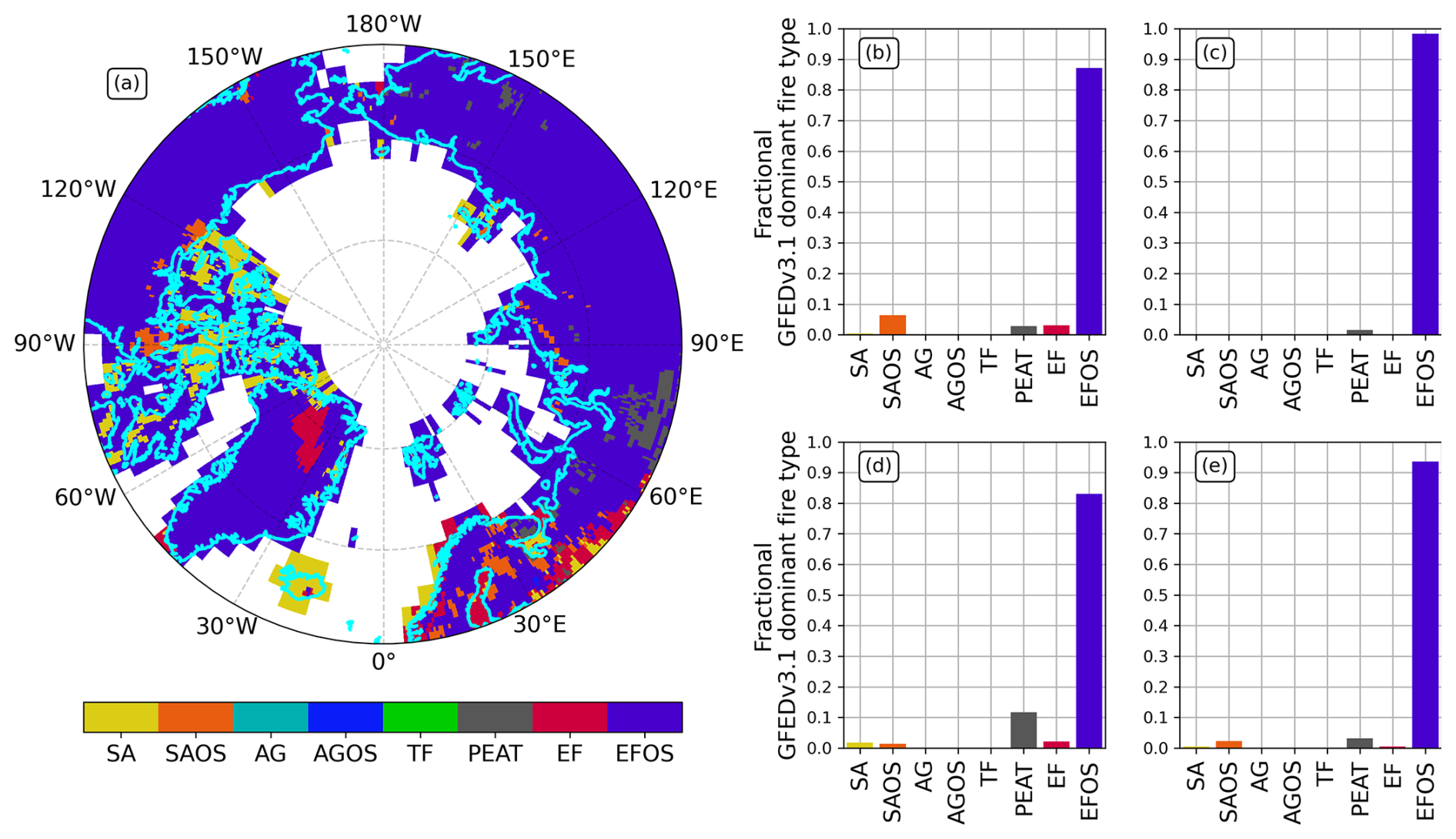
Figure 10 GFAS v1.2 land cover classes, based on dominant fire type in GFED v3.1 and organic soils and peat maps, taken from Kaiser et al. (2012). (a) Land cover classes map, for Savannah (SA), Savannah with organic soils (SAOS), Agriculture (AG), Agriculture with organic soils (AGOS), Tropical Forest (TF), Peat (PEAT), Extratropical Forest (EF), and Extratropical Forests with organic soils (EFOS). 60° N is denoted with a red line. (b–e) Fractional land cover for (b) HL DecNeedle, (c) HL EGNeedle, (d) HL Grassland, and (e) HL Shrubland.

In terms of spatial patterns, Fig. 11 maps the annual total GFAS v1.2 FRE values for the a subregion of the Sakha Republic in Russia in 2021 and the Northwest Territories in Canada 2023 respectively. The elevated annual FRE totals (Fig. 11a and b) align with CO emissions across all four inventories (Fig. 11c–h), whose spatial pattern is very similar, and corresponded to the extreme wildfire activity reported in these years and regions (Byrne et al., 2024; Kharuk et al., 2021). This is to be expected, as HLFREM, FEER-equivalent, and GFASv1.2 emissions all stem from GFASv1.2 FRE totals.

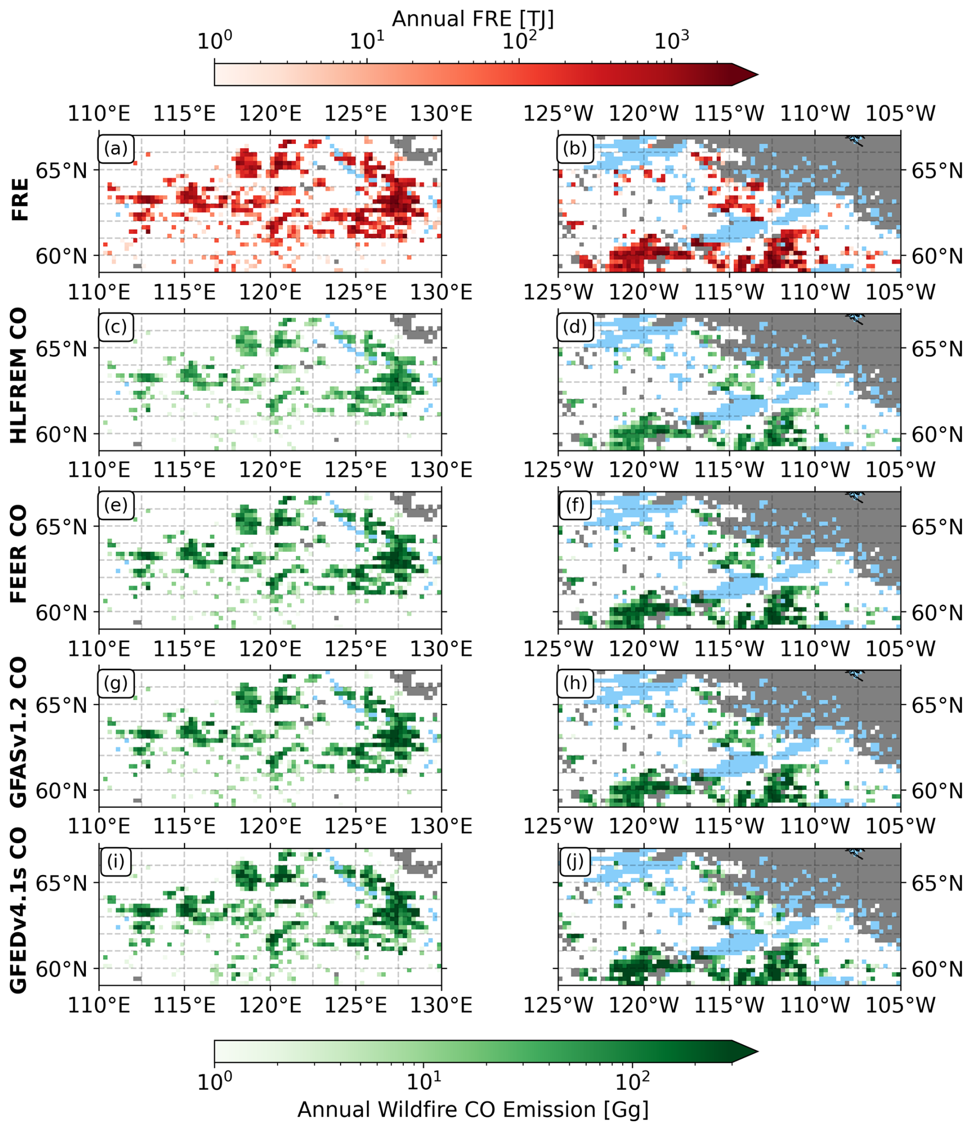
Figure 11 Annual FRE totals from GFAS v1.2 (a, b) and CO emissions (c–j) for a subregion of the Northwest Territories, Canada in 2023 (a, c, e, h, i) and a subregion of the Sakha Republic, Russia in 2021 (b, d, f, h, j) from HLFREM (c, d), FEER-equivalent (e, f), GFAS v1.2 (g, h), and GFED v4.1s (i, j), respectively. Grey areas denote regions that do not fall under one of the four HLFREM biomes, whilst blue denote waterbodies.

4.2 High Latitude Carbon Emission Timeseries

Following the approach of (Mota and Wooster, 2018; Nguyen et al., 2023; Nguyen and Wooster, 2020), emissions estimates of total carbon, as well as any other GHG or trace gas, can be derived from the CO emissions provided by the HLFREM approach, simply via use of standard ratios of the relevant gaseous emission factors. Numerous different summarised EF inventories exist, with for example GFAS v1.2 using (Andreae and Merlet, 2001) and GFEDv4.1s using (Akagi et al., 2011). HL wildfire emissions of Carbon, for example, can be calculated using its biome-specific emission coefficient (${\mathrm{EC}}_{\mathrm{C}}^{\mathrm{b}}),$ derived using the EF ratio between Carbon and CO, and the HLFREM CO emission coefficient$({\mathrm{EC}}_{\mathrm{CO}}^{\mathrm{b}}$), via Eq. (2):

$$\begin{array}{}\text{(2)}& {\mathrm{EC}}_{\mathrm{C}}^{\mathrm{b}}={\displaystyle \frac{{\mathrm{EF}}_{\mathrm{C}}^{\mathrm{b}}}{{\mathrm{EF}}_{\mathrm{CO}}^{\mathrm{b}}}}{\mathrm{EC}}_{\mathrm{CO}}^{\mathrm{b}}\end{array}$$

Where the emission coefficients have units: g MJ⁻¹ and the emission factors units: g kg⁻¹. ${\mathrm{EF}}_{\mathrm{CO}}^{\mathrm{b}}$ values are taken from the aforementioned emission inventories, and ${\mathrm{EF}}_{\mathrm{C}}^{\mathrm{b}}$ being calculated using Eq. (3):

$$\begin{array}{}\text{(3)}& {\mathrm{EF}}_{\mathrm{C}}^{\mathrm{b}}={\displaystyle \frac{\mathrm{12}}{\mathrm{44}}}{\mathrm{EF}}_{{\mathrm{CO}}_{\mathrm{2}}}^{\mathrm{b}}+{\displaystyle \frac{\mathrm{12}}{\mathrm{28}}}{\mathrm{EF}}_{\mathrm{CO}}^{\mathrm{b}}+{\displaystyle \frac{\mathrm{12}}{\mathrm{16}}}{\mathrm{EF}}_{{\mathrm{CH}}_{\mathrm{4}}}^{\mathrm{b}}\end{array}$$

Where ${\mathrm{EF}}_{\mathrm{C}}^{\mathrm{b}}$, ${\mathrm{EC}}_{{\mathrm{CO}}_{\mathrm{2}}}^{\mathrm{b}}$, ${\mathrm{EC}}_{\mathrm{CO}}^{\mathrm{b}}$, and ${\mathrm{EC}}_{{\mathrm{CH}}_{\mathrm{4}}}^{\mathrm{b}}$ are the biome specific wildfire EFs for burnt carbon, CO₂, CO, and CH₄ respectively, assuming these make up more than 95 % of burnt carbon emitted in gaseous form (Akagi et al., 2011) and that by comparison carbon in aerosols is negligible by mass (Akagi et al., 2011; Andreae and Merlet, 2001). Multiplying these carbon emissions by a factor of two then provides an estimate of the amount of biomass burned.

Similar to Fig. 7, Fig. 12 shows our multi-inventory Carbon emissions calculated across the four most dominant HL fire affected biomes. As GFAS v1.2 uses EFs from Andreae and Merlet (2001), we calculated ${\mathrm{EC}}_{\mathrm{C}}^{\mathrm{b}}$ for both HLFREM and FEER using these same EFs, as shown in Table 4. However, as GFED v4.1s uses EFs from Akagi et al. (2011), we also calculated ${\mathrm{EC}}_{\mathrm{C}}^{\mathrm{b}}$ for HLFREM using these same EFs, also shown in Table 4. The HLFREM and FEER ${\mathrm{EC}}_{\mathrm{C}}^{\mathrm{b}}$ were applied to the GFAS v1.2 daily FRE totals, and, similar to Table 6, mean annual HL Wildfire Carbon emissions totals were calculated, and are shown in Table 7.

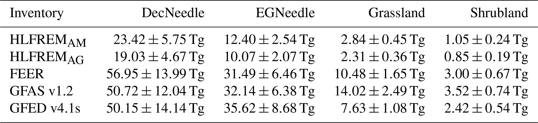
The HLFREM carbon emission timeseries exhibits a very similar behaviour as the CO emission timeseries from which it was derived; with a strong temporal similarity with the carbon emissions of the other inventories. The difference between the HLFREM carbon emissions and the other inventories for the two forested biomes (DecNeedle: 38 %, 30 %, and 42 % smaller than FEER, GFAS v1.2, and GFED v4.1s respectively, EGNeedle: 28 %, 30 % and 42 % smaller than FEER, GFAS v1.2, and GFED v4.1s respectively) and the Shrubland biomes (31 %, 41 %, and 32 % smaller than FEER, GFAS v1.2, and GFED v4.1s respectively), are very similar to those of the CO emissions, differing by ≤2 % from these. The HLFREM carbon emission timeseries from Grassland also exhibits a similar behaviour to those of the Grassland HLFREM CO emission timeseries (65 %, 74 %, and 61 % smaller than FEER, GFAS v1.2, and GFED v4.1s respectively); in that the emission estimations are significantly smaller than those from the other inventories, although the difference from GFAS v1.2 (6 %) is larger than those from the other two inventories (2 %).

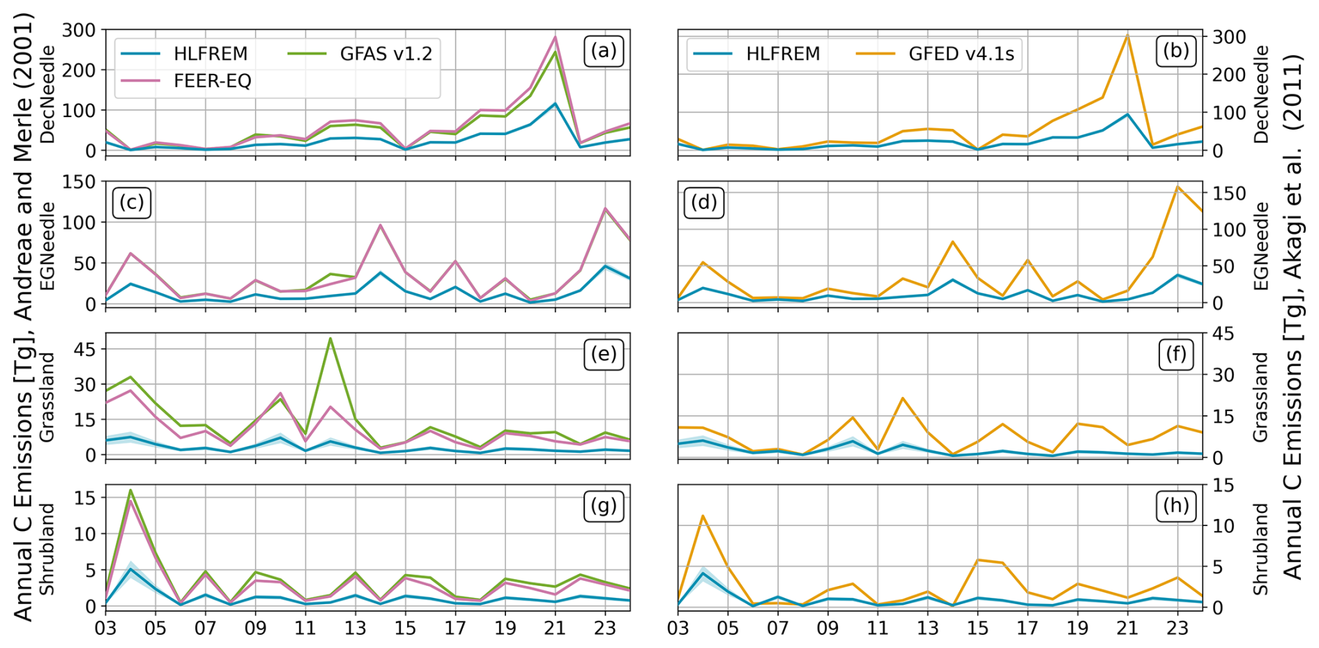
Figure 12 Timeseries of HL Wildfire Emissions of Carbon for (a, b) Deciduous Needleleaf Forest, (c, d) Evergreen Needleleaf Forest, (e, f) Grasslands, and (g, h) Shrublands biomes, for (a, c, e, g) FEER, GFAS v1.2, and HLFREM (using EFs from Andreae and Merlet, 2001), and (b, d, f, h) GFEDv4.1s and HLFREM (using EFs from Akagi et al., 2011). Regression analysis on the timeseries can be found in Fig. A4 in Appendix A.

Table 7 Mean annual (2003–2024) C emissions for the inventory-biome pairs. HLFREM_AM details the mean annual HL Carbon emissions, using EC_C−AM^b, whilst HLFREM_AG details the mean annual HL Carbon emission using EC_C−AG^b. HLFREM and FEER HL Carbon emissions are generated using GFAS v1.2 FRE totals. Uncertainty values are the standard error of the mean.

5 Summary and Conclusions

Taking advantage of the increased number of polar orbiting satellite overpasses nearer the poles, we have extended the Fire Radiative Energy Emissions (FREM) approach to direct “top down” fire emissions estimation to High Latitudes (HL) fires, and to polar-orbiting FRP datasets. Previously the approach was limited to use on low-to-mid latitude geostationary FRP data (Nguyen et al., 2023). This highly direct approach to estimating fire emissions uses only satellite observations of fire radiative power and CO, removing the need for assuming the amount of biomass per unit area, pre-fire fuel loads and combustion completeness, or correlations between FRE and burned biomass developed in the laboratory, in small scale fires, or elsewhere. Negating the requirements for these parameters removes a key source of uncertainty associated with other emissions estimation techniques (Kasischke and Penner, 2004; Reid et al., 2009; Wooster et al., 2015), and provides a means of converting the FRE data from the Global Fire Assimilation system (GFAS) into fire emissions without use of factors derived via linear regressions against the GFED burned biomass totals, as is used currently within GFAS (Kaiser et al., 2012).

Via a set of 708 matchup fires across four regions of interest in the HL region above 60° N, we used S5P TROPMI Total Column Carbon Monoxide (TCCO) data to calculate total plume CO and total FRE up to the time of the S5P overpass from GFAS v1.4. From these data a set of biome specific CO emission coefficients (${\mathrm{EC}}_{\mathrm{CO}}^{\mathrm{b}}$) were generated using the approach of Nguyen et al. (2023) that can then be used to convert further FRP data of fires in the four dominant HL biomes (Deciduous Needleleaf Forests, Evergreen Needleleaf Forests, Grasslands, and Shrublands) to emission rates of CO. Application of these emissions coefficients to the daily FRE totals from GFAS v1.2 enabled us to produce new CO emissions inventory for these four biomes in the HL region, unreliant on any additional parameters or datasets.

The CO emissions derived from this new approach were compared to three other widely used fire emission inventories, those produced and outputted by GFAS v1.2 itself, those from FEERv1.0-GFASv1.2 (calculated using GFAS FRE and a FEER-equivalent ${\mathrm{EC}}_{\mathrm{CO}}^{\mathrm{b}}$; Nguyen et al., 2023), and those from GFED v4.1s. Total carbon emissions estimates were also calculated based on emission factor ratios between CO and Carbon. The HLFREM CO and Carbon emissions timeseries and CO spatial patterns derived using the HLFREM approach were found to be in good temporal and spatial agreement with the FEER-equivalent, GFAS v1.2, and GFED v4.1s inventories, particularly for the two forested biomes and shrublands, producing relatively similar but generally smaller emissions totals. Mean annual HLFREM CO and carbon emission totals were found to be 54 %–71 % smaller than totals produced by FEER, GFAS v1.2, and GFAS v4.1s for the two forested biomes and Shrubland biomes. HLFREM CO and carbon emission totals from Grassland were also in good temporal and spatial agreement with the other inventories, although the emissions were significantly lower (71 %–85 %) than those from other inventories; and whilst this could be correct, it is also possibly a result of the relatively small number of fire-matchups found during the generation of the HLFREM ${\mathrm{EC}}_{\mathrm{CO}}^{\mathrm{Grassland}}$ and perhaps a low bias. Compounding this, the largest difference (GFAS v1.2, 85 % lower CO emissions, 80 % lower carbon emissions) was found over the Grassland biomes, which in certain of the other databases has some consideration of peat burning included that is not accounted for in the HLFREM methodology.

Not accounting for peat burning, as well as not accounting for changes in combustion phase, by assuming a single relationship between CO emissions and FRE within each fire biome is a limitation of this HLFREM methodology. While combustion phase cannot be currently be resolved using space-based EO observations, organic soil content was evaluated as an additional classification variable but was not incorporated because it substantially reduced the sample size within each class.

Future developments in advancing the HLFREM approach will include consideration of this organic soil burning, as well as expansion of both the biomes covered and the number of fire matchups in each. Our aim is to develop a long-term and geographically continuous HL fire emissions dataset that does not rely on parameters taken from modelling, from correlations between inventories, or from conversion coefficients taken from laboratory or small-scale fire experiments when converting the satellite observations into emissions estimates. Instead, the FREM approach uses information extracted from the satellite data itself to generate the necessary conversion coefficients, an approach that we feel has great potential to expand further as both active fire and trace gas remotely sensed datasets continue to advance.

Whilst the HLFREM framework is readily transferable to fires globally, through a global matchup fire database using TROPOMI TCCO observations and a global GFAS v1.4 dataset, its application would likely benefit more from the use of geostationary FRP observations from other platforms, such as the National Oceanic and Atmospheric Administration (NOAA) Geostationary Operational Environment Satellite (GOES) or Japan Aerospace Exploration Agency (JAXA) Himawari platforms, where available. Compared to with the hourly GFAS FRP product, which relies on a prescribed diurnal cycle (Andela et al., 2015) to distribute fire activity between solar overpasses, geostationary observations provide much higher temporal resolution, and directly capture the natural diurnal variability of fire behaviour. This would allow the temporal evolution of emissions to be represented more realistically, particularly for fires with rapidly changing intensities.

Appendix A

Table A1 Aggregated CCI landcover classes (taken from ESA 2017) assigned to each HLFREM biome.

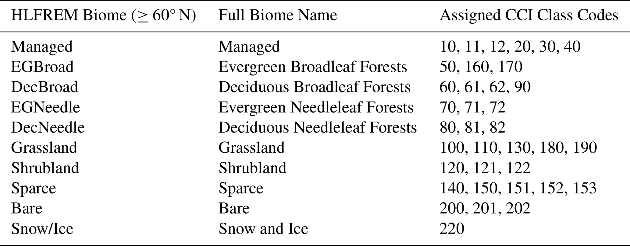
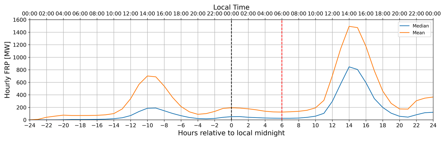
Figure A1 Median (blue) and mean (orange) hourly FRP of all plumes identified in the HLFREM study, during the day before observation (negative hours relative to local midnight) and day of observation (positive hours relative to local midnight) from the hourly FRP dataset. Local midnight and 06:00 local time is shown with the black and red line, respectively.

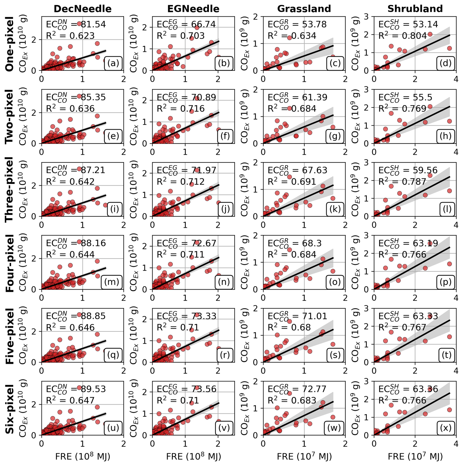
Figure A2 HLFREM biome-specific CO emission coefficients (${\mathrm{EC}}_{\mathrm{CO}}^{\mathrm{b}}$, in g MJ⁻¹) derived for Deciduous Needleleaf Forests (DecNeedle, a, e, i, m, q, u), Evergreen Needleleaf Forests (EGNeedle, b, f, j, n, r, v), Grassland (Grassland, c, g, k, o, s, w), and Shrubland (Shrubland, d, h, l, p, t, x), using a one- (a, b, c, d), two- (e, f, g, h), three- (i, j, k, l), four- (m, n, o, p), five- (q, r, s, t), and six-pixel buffer (u, v, w, x) to determine the background TCCO values, used in Table 5. R² values are also shown.

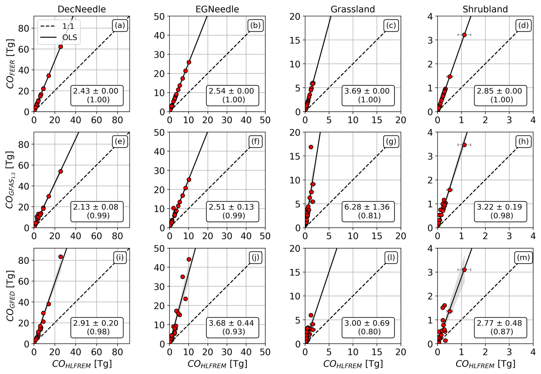
Figure A3 OLS Regression analysis of the Annual HL CO Emissions, comparing the HLFREM emissions (calculated using GFAS v1.2 FRE totals) with (a–d) FEER, (e–h) GFAS v1.2, and (i–l) for Deciduous Needleleaf Forests (a, e, i), Evergreen Needleleaf Forests (b, f, j), Grassland (c, g, k), and Shrubland (d, h, l) biomes. OLS regression and associated errors are shown on each plot (displayed as the solid line and shading respectively), with the R² value being shown in the brackets. A 1:1 line (dashed line) is also shown.

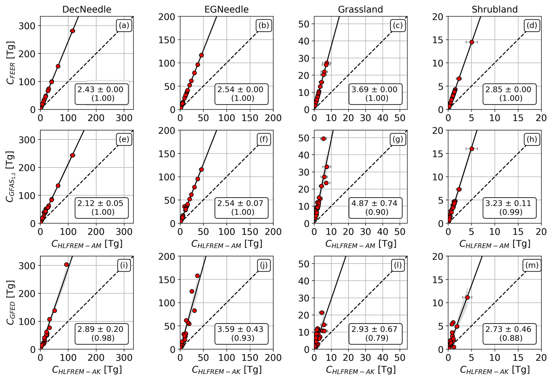
Figure A4 OLS Regression analysis of the Annual HL C Emissions, comparing the HLFREM emissions (calculated using GFAS v1.2 FRE totals) with (a–d) FEER, (e–h) GFAS v1.2, and (i–l) for Deciduous Needleleaf Forests (a, e, i), Evergreen Needleleaf Forests (b, f, j), Grassland (c, g, k), and Shrubland (d, h, l) biomes. As the HLFREM C Emissions have been calculated via EF ratios with respect to Carbon Monoxide, different EF ratios have been used to compare FEER and GFAS v1.2 (using EFs from Andreae and Merlet, 2001, referred to as HLFREM_AM), and GFEDv4.1s (using EFs from Akagi et al., 2011, referred to as HLFREM_AG). OLS regression and associated errors are shown on each plot (displayed as the solid line and shading respectively), with the R² value being shown in the brackets. A 1:1 line (dashed line) is also shown.