How beech ecophysiology shapes temperate forest gross primary productivity – Part 1: A wavelet-based framework for extracting seasonal dynamics

Long-term eddy covariance (EC) records provide unique opportunities to investigate how seasonal carbon dynamics shape interannual and decadal trends in forest carbon uptake. Yet extracting reproducible phenological and structural information from noisy, non-stationary gross primary productivity (GPP) time series remains challenging. Here we present a wavelet-based analytical framework that directly exploits the time-frequency structure of GPP signals to identify repeated seasonal features. This approach departs from standard wavelet applications by analyzing the full set of wavelet coefficients as an interpretable structure to systematically detect and characterize recurrent patterns, including moderate-amplitude events that are typically overlooked by significance-based or visually driven wavelet analyses. Building on this foundation, we introduce a novel Wavelet Area Interpretation (WAI) method that extracts three complementary indicators of seasonal GPP dynamics (IRise for rising rate; IPeak for peak productivity; IDrop for mid-season decline) and derives carbon-uptake phenological markers within a unified workflow. Together, these metrics provide a coherent representation of the timing, magnitude and shape of the seasonal GPP cycle. We apply this framework to long-term EC records from three contrasting ICOS-labelled European beech-dominated forests (DE-Hai, DK-Sor, FR-Hes), demonstrating its ability to reveal both structural differences among sites and divergent long-term trajectories in carbon uptake. Benchmarking against classic smoothed GPP reference values confirms the robustness of IRise and IPeak and clarifies the inherent uncertainties associated with mid-season metrics. Ecologically, the indicators uncover consistent contrasts in seasonal structure: rapid spring rise at FR-Hes, muted mid-season decline at DK-Sor, and early cessation of uptake at DE-Hai. They reveal opposing multi-decadal trends, with peak productivity increasing in the managed stands but declining in the unmanaged old-growth forest. The negative association between IRise and mid-season drop timing further suggests an intra-seasonal trade-off linking early-season vigor to mid-season susceptibility. Overall, this study provides a novel, scale-aware approach for extracting seasonal information from noisy time series and demonstrates how WAI-derived indicators can yield new insights into the mechanisms driving long-term variability across sites and applications.

1 Introduction

The past century has seen remarkable advancements in measurement and communication technologies, fostering the growth and maturity of various research domains (Krapivin and Shutko, 2012; Pandey and Sharma, 2021; Trankler and Kanoun, 2001). Among these, the increasing availability of long, high-frequency environmental time series has transformed ecosystem science, enabling the investigation of biological and climatic processes across a wide range of temporal scales (Allan et al., 2018; Krapivin et al., 2015; Marvin et al., 2016). At the same time, this “data-rich” context poses an analytical challenge: extracting interpretable and reproducible information from signals that are inherently noisy, often non-stationary, and shaped by overlapping processes (e.g., seasonality, trends, extremes, and legacy effects) (Ascough et al., 2008; Oliveira et al., 2012; Reichman et al., 2011).

Methods designed to decompose time series into components operating at different temporal scales have therefore become central to contemporary environmental research (Platt and Denman, 1975). Spectral analysis based on the Fourier transform (FT) remains foundational for characterizing the frequency content of a signal (Percival and Walden, 1993). However, the FT represents a signal in the frequency domain without explicit time localization, which makes it less suited for detecting time-localized events (e.g., abrupt changes, short-lived anomalies, or irregular seasonal disturbances) that can be ecologically meaningful (Debnath and Shah, 2015; Farge, 1992). This limitation has motivated the development and adoption of time-frequency methods in which information is jointly represented in time and in frequency (or scale). Wavelet transforms (WT) provide such a representation by convolving the signal with localized analyzing functions (wavelets) across scales, thereby enabling the study of how dominant modes of variability evolve through time (Mallat, 2009).

Because many ecological and environmental time series are non-stationary and contain transient or discontinuous components, the WT has become an established tool in ecology and Earth sciences (Moreaux et al., 2020). Wavelet analysis is now used to study a broad range of processes, from population cycles (Hudson et al., 2011) to climate-ecosystem couplings (Carl et al., 2013), precisely because it can isolate variability at specific time scales while preserving temporal localization. Practical guides and standardized toolkits, most notably Torrence and Compo (1998), have facilitated the diffusion of wavelet methods beyond specialist communities, including the formalization of commonly used significance testing procedures based on idealized noise backgrounds. Yet, despite this success, wavelet analyses in ecology often rely on a limited subset of coefficients or summary diagnostics, with methodological choices (wavelet family, normalization, thresholding, and significance conventions) frequently inherited from precedent rather than tailored to the signal features of interest (e.g., Carl et al., 2013; Moreaux et al., 2020; Schaller et al., 2017). This can bias interpretation toward only the most prominent patterns and may obscure repeated but moderate-amplitude events that nevertheless carry strong ecological meaning.

These methodological questions are particularly relevant for ecosystem carbon-cycle studies based on eddy covariance (EC) data. EC time series provide continuous observations of net ecosystem exchange (NEE) and derived flux components such as gross primary productivity (GPP), enabling mechanistic investigations of seasonal carbon dynamics and their sensitivity to climate (Aubinet et al., 2012). However, extracting phenological transition dates and seasonal features from EC-derived GPP remains challenging because daily flux signals are noisy and site-specific seasonal shapes can differ substantially (Moffat et al., 2007). Recent syntheses show that different smoothing choices and phenology extraction methods (e.g., threshold versus derivative approaches) can shift inferred start and end of season dates by weeks, which in turn affects trend estimates and cross-site comparisons (Panwar et al., 2023). These uncertainties are exacerbated at sites where seasonal transitions are gradual, where growing seasons are asymmetric, or where multiple intra-seasonal perturbations occur (Xie et al., 2023).

In European temperate forests, these challenges intersect with a pressing ecological question: how do seasonal GPP dynamics and carbon uptake phenology shape long-term forest carbon sequestration? European beech (Fagus sylvatica L.) forests are central to this question because they dominate large areas of Central and Western Europe (Chiesi et al., 2016) and have shown pronounced sensitivity to drought and heat, with impacts including reduced photosynthetic activity, early senescence, and legacy effects after severe events (Campioli et al., 2011; Hesse et al., 2023; Leuschner, 2020). Meanwhile, multi-decadal EC records indicate that carbon uptake trajectories can differ markedly among beech-dominated stands, reflecting interactions among climate regime, stand age, and management (Gennaretti et al., 2020; Kulla et al., 2023; Xiao et al., 2026). Understanding such contrasts requires metrics that go beyond simple seasonal integrals, and that explicitly quantify seasonal structure, e.g., the spring rise, the peak assimilation capacity, and the extent of mid-season depression.

Here we propose and apply a wavelet-based framework designed to address two related limitations in current practice: (i) the tendency to focus on a restricted subset of prominent wavelet outputs and (ii) the reliance on significance testing frameworks that may discard relevant coefficients when the assumed noise background is not appropriate (Cazelles et al., 2014). Building on the mathematical structure of the WT and its time-scale localization properties, we introduce an alternative perspective that treats wavelet coefficients as a systematic basis for detecting repeated events in non-stationary signals, rather than as isolated features evaluated primarily through statistical significance maps. The method will be illustrated using 20 years of the FR-Hes GPP signal. This choice stems from the signal's shape, characterized by well-marked diurnal and annual trends (Fig. S1), and the availability of decade-long datasets through international networks such as ICOS, NEON or FLUXNET. Both characteristics tend to complicate classical WT analyses, providing an effective illustration of the benefits of our approach.

From this framework, we derive indicators that summarize the seasonal structure of GPP and carbon-uptake phenological metrics. Because phenological inference from EC data can be method-dependent, we explicitly benchmark these indicators and phenological dates against estimates derived directly from smoothed GPP seasonal curves. We apply this methodology to three long-term beech-dominated EC sites DE-Hai (Hainich, Germany), DK-Sor (Sorø, Denmark) and FR-Hes (Hesse, France). These forests differ in management history, age structure, and climatic setting, providing an ideal testbed to evaluate whether wavelet-derived seasonal indicators and phenological metrics capture consistent ecological contrasts and whether site differences remain stable or change through time.

Specifically, our objectives are to: (1) evaluate the consistency of the wavelet-based indicators and phenological metrics through benchmarking against smoothed-GPP reference metrics; (2) quantify long-term trends in annual carbon fluxes and in seasonal-structure indicators; and (3) test for systematic differences among sites and for potential temporal changes in these differences using linear mixed-effects models that account for shared year-to-year anomalies. In doing so, we aim to provide (i) a methodological contribution: an operational, interpretable wavelet-based event detection and interpretation strategy, and (ii) an ecological contribution: new comparative insight into how seasonal GPP structure and carbon-uptake phenology differ among long-standing beech-dominated forests across Europe.

2 Methods

2.1 Theoretical background

The wavelet transform (WT) can be perceived as an extension of the Fourier transform (FT). Both can be expressed as an inner product between a function of interest f(x) and analyzing functions, all of which are derived from a single mother function (Mallat, 2009). The distinction between both transforms arises from the properties of these analyzing functions, described hereafter.

• The FT employs sine and cosine waves, which can be expressed as complex exponentials (Fig. 1a). These functions are periodic, implying that their spread encompasses the entirety of the x-axis. They depend solely on a single parameter, the frequency. Consequently, we can only extract a global coefficient for each frequency, representing the influence of this frequency component on the entire function. The coefficients are necessarily complex-valued and can be associated with a phase (which part of the sine and cosine yields the information) and an amplitude (importance of the frequency component in the function). The amplitude of the Fourier coefficients is represented for each frequency (or period) in a 2-dimensional graph, known as periodogram (Fig. 1c).

• The WT relies on oscillating and (approximately) compact functions, aptly named “wavelets” (Fig. 1b). These analyzing functions are concentrated on a finite portion of the x-axis, referred to as the support of the wavelet, and can be translated to cover the whole x-axis. To detect oscillatory behavior in f(x), the wavelets are scaled to match a corresponding frequency. Therefore, wavelets depend on two parameters: the center of the x-axis portion where the wavelet spans (position or time, for time-varying functions) and the scale of the wavelet (frequency). Wavelets can be real or complex, and so are the coefficients for real functions f(x). The amplitude of wavelet coefficients is represented for each couple time-frequency (or time-period) in a 3-dimensional graph, called scalogram (Fig. 1d).

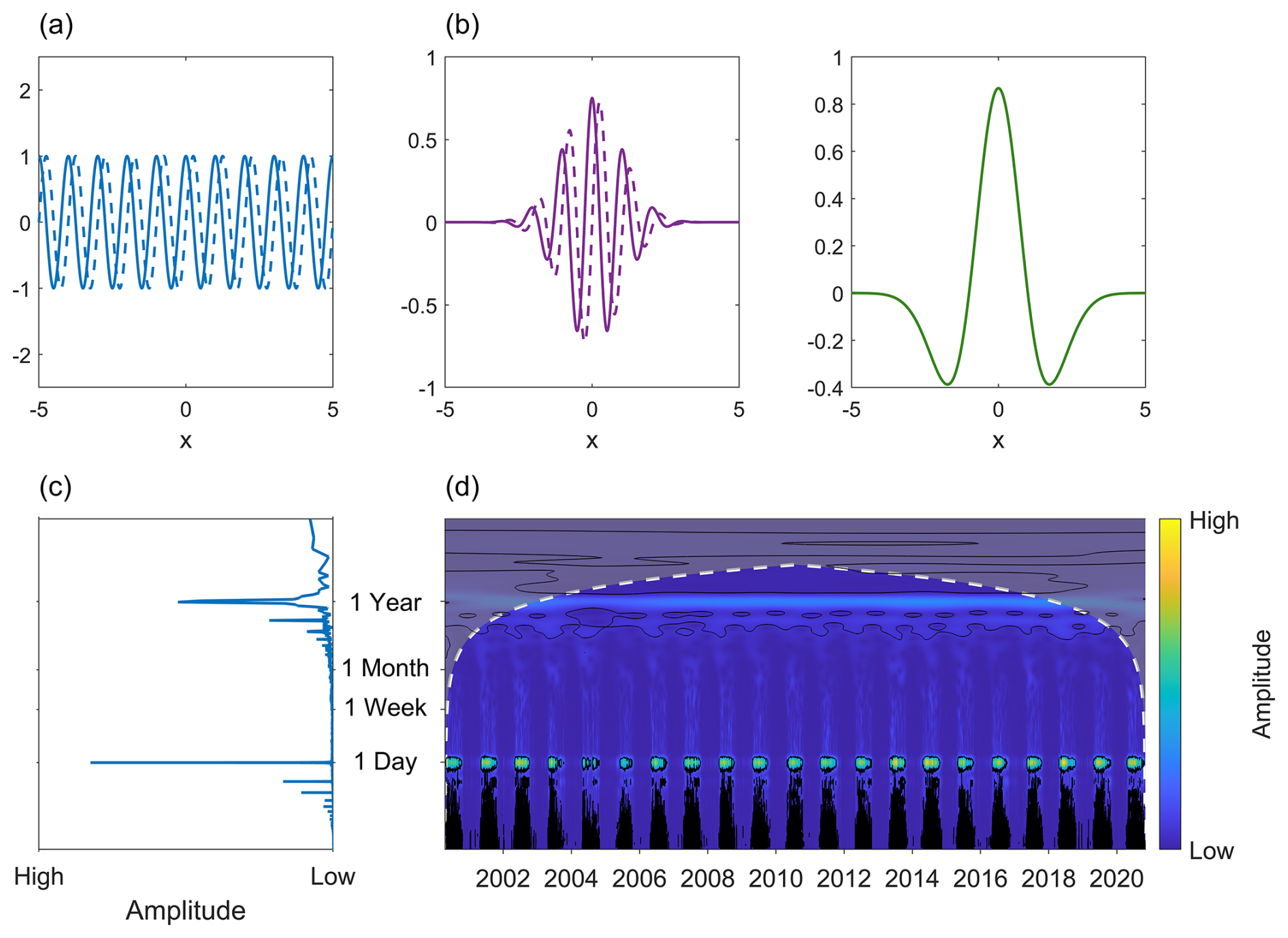
Figure 1 Graphical difference between the FT and WT. (a) Analyzing functions of the FT: sine and cosine waves, (b) Analyzing functions for the WT: Morlet wavelet (left, real and imaginary part distinguished by solid and dashed lines) and Mexican Hat wavelet (right), (c) Periodogram of the 2000–2020 FR-Hes GPP signal. The y-axis is in logarithmic scale, (d) Scalogram of the 2000–2020 FR-Hes GPP signal using the Morlet wavelet. The y-axis is in logarithmic scale. Shaded areas represent coefficients affected by edge effects, delimited by the cone of influence (Sect. S1) in white dashes. Statistically significant coefficients, assuming a red background noise, are contoured in black.

These descriptions provide an intuitive understanding of how both transforms extract oscillatory behaviors from a function: if f(x) oscillates at a certain frequency, it will align well with the sine/cosine functions or the wavelet at the same frequency, leading to elevated coefficients. Conversely, in the absence of, or in the presence of minimal fluctuations in f(x) at a specific frequency, the coefficients will approach zero, reflecting the dissimilarity between f(x) and the analyzing functions. The WT, however, addresses limitations of the FT by constraining the spread of its analyzing functions, thereby enabling the study of non-stationary behaviors. Although both transforms preserve all information from f(x), the FT disperses it along the infinite fluctuations of its sine/cosine waves, disabling any possibility of localization (Debnath and Shah, 2015; Farge, 1992).

The WT can be either continuous or discrete, with the difference lying in the permissible values for the parameters of the analyzing functions. In the continuous case, wavelets are allowed to translate across all x values, even if they overlap, and the scales of the wavelets can vary continuously, leading to redundant information on adjacent scales. The discrete transform eliminates this redundancy by restricting the set of allowable scales and translations (Abbate et al., 2002). This paper concentrates solely on the continuous wavelet transform (CWT) due to its suitability for graphical representations. The scalogram in Fig. 1d results from such a continuous transform, with the Morlet wavelet as analyzing function.

An essential part of a wavelet analysis resides in the selection of the wavelet for the transform. The fundamental principle guiding this process is that the chosen wavelet should bear significant similarities with the trends sought in the signal (Farge, 1992). Several wavelets have previously found success in ecological studies. Torrence and Compo (1998) list, for complex-valued functions, the Morlet and Paul wavelets and, for real ones, the Haar wavelet and a family of wavelets obtained by taking successive derivatives of the Gaussian function. By convention, these last functions are abbreviated as “DOG” followed by the order of derivation of the Gaussian function. For example, the DOG2 wavelet is the second derivative of the Gaussian function and corresponds to the opposite of the Mexican Hat wavelet. The Morlet and Mexican Hat wavelet are the most widespread wavelets used and hence have been illustrated in Fig. 1b. The other wavelets are illustrated in Fig. S2.

For a more comprehensive understanding of the FT and WT, one can refer to the works of Bracewell (2000), Abbate et al. (2002), and Mallat (2009).

2.2 Wavelet Area Interpretation: a novel approach for interpreting wavelet coefficients

When interpreting WT outputs, high coefficient amplitude is typically ascribed to the presence of an oscillatory behavior at corresponding frequency and time in a signal. In the case of the FR-Hes dataset, the GPP scalogram displays high coefficients around a 1-year period (Fig. 1d). This reflects the annual periodicity of the forest's photosynthetic behavior due to climatic (annual course of the sun) and physiological (seasonality of leaves) factors. The daily period band exhibits even higher coefficients concentrated each year during the forest's growing season (GS), mirroring the response of chlorophyl elements to the daily course of incoming photosynthetic radiation when leaves are present. While this approach leads to straightforward interpretations for pronounced trends, it proves impractical for intermediate scales, ranging between a day and a year. Coefficients in these scales occur within narrow time ranges, which can obscure the distinction of underlying phenomena and potentially cause confusion between them. Normalizing the scalogram (see Fig. S3) highlights recurring elevated coefficients in these ranges each year, although they do not always appear significant.

To fully leverage these less-pronounced but information-dense regions of the scalogram, we propose a novel interpretation of wavelet coefficients, based on a mathematical perspective. This approach relies on the definition of the CWT. Considering a time-varying signal x(t) and a wavelet ψ(t), the CWT is expressed as:

$$\begin{array}{}\text{(1)}& \begin{array}{l}W\left(a,b\right)=\underset{-\mathrm{\infty }}{\overset{+\mathrm{\infty }}{\int }}x\left(t\right)\stackrel{\mathrm{‾}}{{\mathit{\psi }}_{a,b}}\left(t\right)\mathrm{d}t\end{array}\end{array}$$

Where the overbar denotes the complex conjugate and ψ_a,b(t) is the wavelet taken at a certain scale a and time b, normalized by introducing a multiplying factor. Since our approach only requires qualitative results, this factor is omitted from further developments. According to the CWT formula, a wavelet coefficient W(a,b) may be constructed by following three steps:

1. Computing the chosen wavelet at scale a and position b, i.e. ${\mathit{\psi }}_{a,b}\left(t\right)=\mathit{\psi }\left(\frac{t-b}{a}\right)$

2. Defining a product curve by multiplying x(t) with (the complex conjugate of) the wavelet.

3. Computing the area under the product curve by positively accounting for contributions that lie above the t=0 axis and negatively for those below.

Figure 2 demonstrates these steps for the Mexican Hat wavelet placed at the start of April with a scale corresponding to a period of 6 months (see Fig. S4 for an example using a complex wavelet). The primary advantage of this graphical approach, named the Wavelet Area Interpretation (WAI), lies in the ability to assign an interpretation to a wavelet coefficient based on the areas contributing to its calculation. For instance, the value of the coefficient computed in Fig. 2 is governed by the third (negative) lobe of the wavelet. Graphically, the projection of the function on this lobe expresses the rising GPP values during the first peak of photosynthetic activity from May to July.

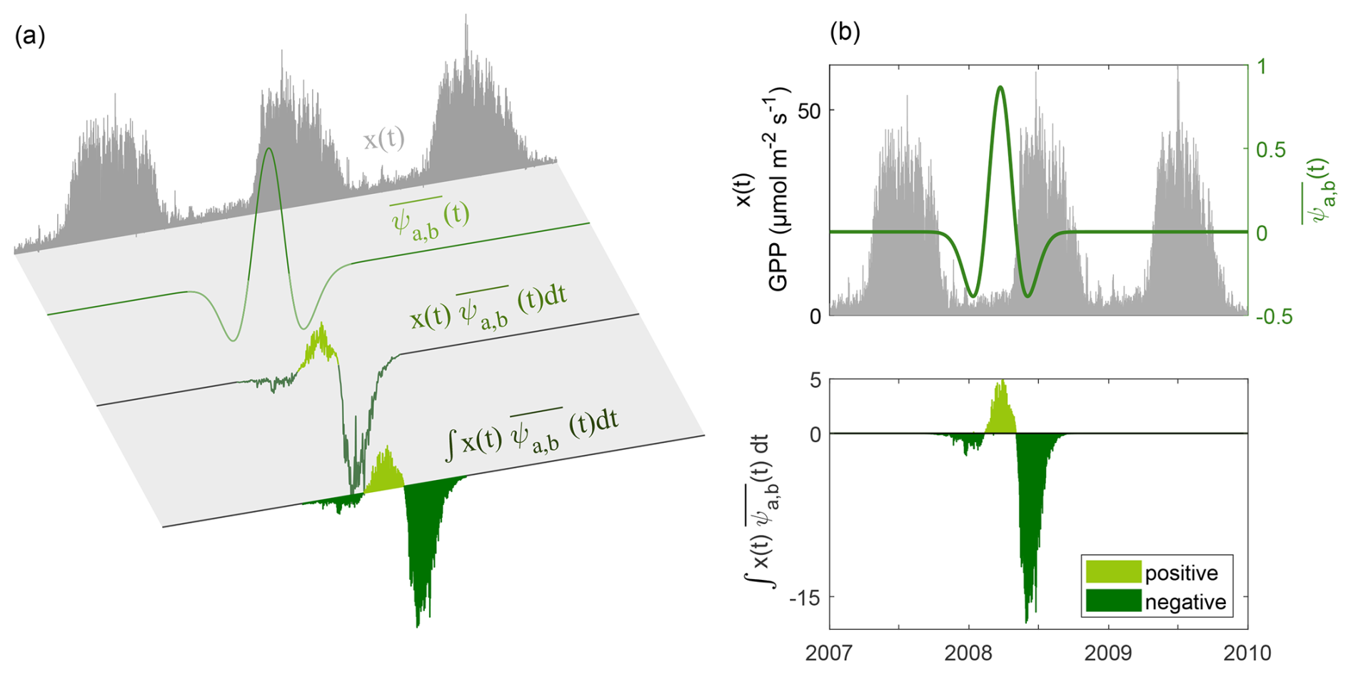
Figure 2 (a) Detailed computation of a wavelet coefficient following the mathematical definition of the CWT. (b) Condensed view of the computation process. The top graph displays the Mexican Hat wavelet at a chosen scale (corresponding to a 6-month period) and time (start of April) with the GPP signal in the background (restricted to positive values for readability). The graph below illustrates the area under the product curve of the wavelet and the signal. The algebraic sum of the three contributing areas, each linked to a lobe of the wavelet, corresponds to the wavelet coefficient yielded by the WT at the selected scale and time, after normalization.

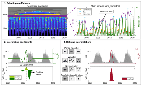
WAI allows for the interpretation of individual wavelet coefficients, but selecting which coefficients to analyze among the plethora generated by the WT is non-trivial and depends on the signal structure. Furthermore, because the contributing areas of a coefficient are determined by the wavelet shape, the interpretability of coefficients varies among wavelets. These considerations highlight the need to integrate WAI into a reproducible, systematic procedure. To this end, we introduce a 3-step method (Fig. 3) for identifying and interpreting meaningful coefficients.

1. Selecting coefficients. Relevant coefficients are identified by representing average period bands as a function of time. For a given period, the mean amplitude of coefficients within a narrow scale range is computed, and local maxima in this period-band signal indicate time windows where prominent patterns occur. These maxima then serve as the primary candidates for WAI interpretation. Wavelet choices for computing period bands are discussed in Sect. S2.

2. Interpreting coefficients. After selecting relevant coefficients from identified peaks, WAI is used to interpret them based on the most prominent contributing areas (see the procedure detailed in Fig. 2).

3. Refining interpretations. To reduce uncertainties in interpretations given to wavelet coefficients, the third step involves adjusting the WT to align coefficient values with interpretations. A wide variety of possibilities exist, among which four are detailed in Sect. S3. The final coefficient value obtained post-adjustments serves as an indicator of the importance of a feature's presence in the signal. Consequently, we simply refer to these values as “indicators”.

Figure 3 Schematic view of the 3-step workflow used to identify and interpret meaningful wavelet coefficients. Step 1 (selection): relevant coefficients are first identified by analyzing the temporal evolution of period-band amplitudes. Local maxima (peaks) in these signals indicate time windows where recurrent seasonal features are present. Step 2 (interpretation): selected coefficients are then interpreted using the WAI, which links each coefficient to the dominant areas of interaction between the wavelet and the signal, allowing direct attribution to specific signal features. Step 3 (refinement): the wavelet transform is adjusted (e.g. wavelet type, period, normalization or coefficient combination) to align coefficients more closely with their intended interpretation and reduce uncertainty. The resulting values are used as indicators of the importance of specific seasonal features. Together, these steps provide a structured and reproducible framework for extracting ecologically meaningful information from complex, non-stationary signals.

These guidelines are designed to integrate the newly introduced WAI approach with classical wavelet analyses by building on familiar WT outputs. They can further be adapted to specific datasets, which is done here for temperate deciduous forest GPP using the FR-Hes site as a case study. In this application, we focus on the DOG family of wavelets (Fig. S1) given their widespread use and extensive documentation, as well as their simple, easily interpretable shapes. Moreover, their weighting structure (positive and negative lobes) can be visually related to specific signal features.

Ready-to-use Python and Matlab codes are available online and all figures were produced using Matlab R2022a (The MathWorks Inc, 2022).

2.3 Application to temperate deciduous forest GPP

2.3.1 Selecting coefficients

Figure 4 demonstrates the 6-month ± 15 d band for the Morlet and Mexican Hat wavelets. Both curves exhibit multiple peaks, offering a variety of relevant choices for further investigation. A closer examination of the Mexican Hat curve can further refine this selection: the 6-month band displays three recurring peaks for each year, in April, June and November (Fig. 4, Zoom).

Figure 4 Amplitude of the wavelet coefficients using the Morlet wavelet (purple) and the Mexican Hat wavelet (green) at the 6-month period band. Grey dashed curves represent coefficients affected by edge effects. Corresponding graph for the 2-month period band is given in Fig. S5.

All three peaks are positioned at key periods of the GPP curve: the onset of rising values in April (second zero of the wavelet, Fig. 5a), the GPP peak in June (maximum of the wavelet, Fig. 5b) and the end of decreasing values in November (first zero of the wavelet, Fig. 5c). This repeated behavior hints at the ability of these peaks to extract specific features pertaining to the annual pattern of the GPP curve for temperate deciduous forests.

The GPP scalogram displays significant coefficients for a range of periods, from 6 months to 1–2 months (Fig. 1d). Building on the wavelet positioning for the annually recurring 6-month peaks, the corresponding 2-month peaks were identified using the WAI (Fig. 5d–f), resulting in 6 selected peaks per year.

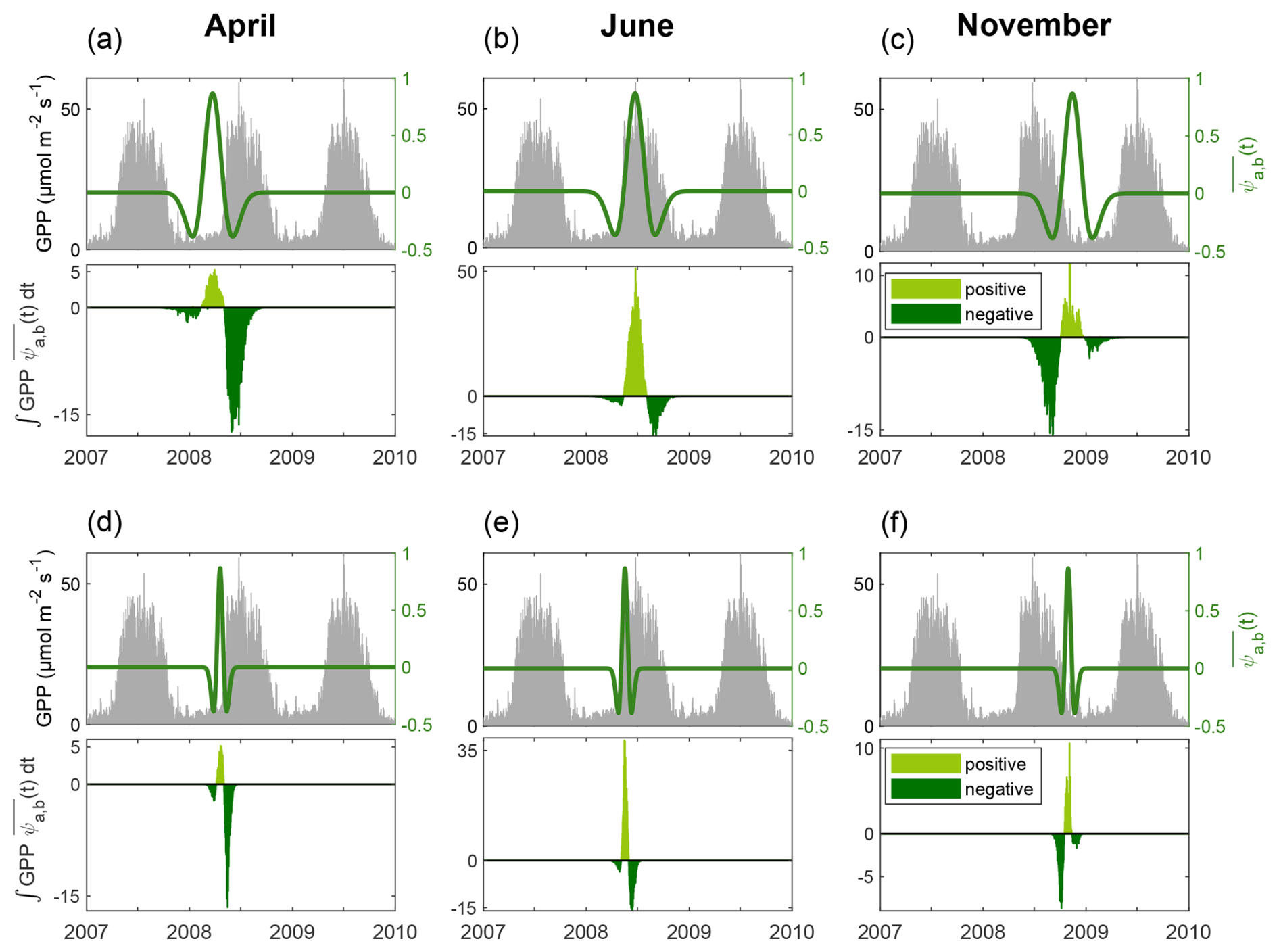
Figure 5 Computation steps for wavelet coefficients, (a–c) at a 6-month period for the three annual peaks observed with the Mexican Hat wavelet (see Fig. 4, zoom), and (d–f) at a 2-month period for their low-period counterpart.

2.3.2 Interpreting coefficients

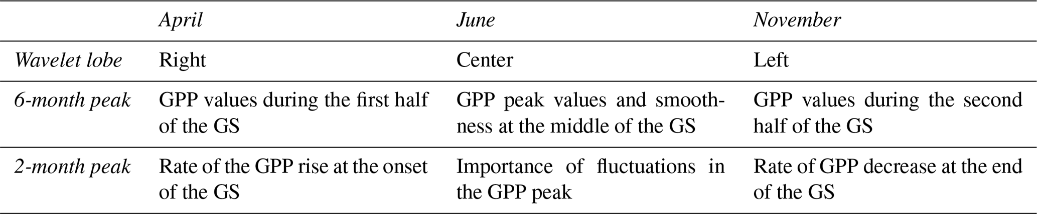
Based on areas that contribute most strongly to coefficient values, contrasting interpretations can be attributed to these three pairs of peaks. They are summarized in Table 1.

At a 6-month period, the April peak value is primarily influenced by the right lobe of the wavelet. The wavelet serves as a weighting factor, yielding high coefficients if the GPP signal reaches high values during the first half of the GS. The 2-month period focuses on the rising phase of the GPP at the onset of the GS. It will thus depend on the rate at which the forest's photosynthetic activity reaches its maximum values. The central lobe acts as an inverse weighting factor in case of a progressive GPP increase.

The June peak value is derived from the central part of the wavelet. At a 6-month period, its value increases if the initial GPP peak reaches high values and maintains global smoothness, with minimal to no significant summer drops. Ideally, GPP follows a bell-shaped curve during the first half of the GS (Fig. S1) when environmental stresses are scarce. The intensity of this peak is directly related to limiting factors on leaf cover density, such as biotic stresses, winter thinning or lacking nitrates or starch reserves. The 2-month period is of less interest. It can be associated with the presence of high amplitude fluctuations in the initial GPP peak, as can result from storms or weather fronts.

The November peaks are symmetrical to the April ones, with the left lobe of the wavelet extracting the feature. Consequently, the 6-month peak represents the GPP values during the second half of the GS, marked by reduced photosynthetic activity due to dwindling incoming photosynthetic radiation. Environmental stresses, predominantly aerial or edaphic drought, can drastically accentuate this drop starting mid-July. The 2-month peak translates the rate of the GPP decline due to senescence. Similar to the April peak, the center lobe can negatively impact the 2-month coefficient if the decrease in GPP is gradual.

Table 1 Lobe of the Mexican Hat wavelet extracting information and associated interpretations for high-period (6 months) and low-period (2 months) peaks in wavelet coefficients.

2.3.3 Indicators

Using the interpretations summarized in Table 1, we defined three indicators describing key seasonal features of the GPP cycle, incorporating the adjustments detailed in Sect. S3. Their construction relies on targeted use of wavelet coefficients at specific scales, selected to match the temporal processes of interest. These indicators were designed to capture three main, well-documented phases of seasonal GPP dynamics in temperate deciduous forests, providing a coherent and complementary description of seasonal dynamics while remaining robust and interpretable across sites. Additional candidate indicators are presented in Sect. S4 but were not retained for further analysis due to low ecophysiological relevance, reduced signal detectability or redundancy with the selected indicators.

• 1.

  IRise: Spring rising rate

  IRise quantifies the rate at which GPP increases from the start of the GS to its seasonal maximum. The low-period April peak identified in Table 1 reflects this early-season rise.

  • Wavelet selection: The Mexican Hat wavelet introduces unwanted contributions from its left and central lobes (Fig. 5d). To avoid these effects, we use the DOG1 wavelet, which consists of two symmetric lobes. The left lobe acts as a negative weight during the early increase, and the right lobe isolates upper GPP values during the first half of the season (Fig. 6a).

  • Signal normalization: Prior to transformation, GPP is normalized by its annual amplitude to remove sensitivity to interannual changes in absolute GPP levels.

  • Period adjustment: The DOG1 scale is chosen to match the approximate 2-month duration required for GPP to reach its peak under favorable conditions. Considering an average 12 d offset between the wavelet positioning and the start of the GS (evaluated using phenological data), the right lobe should instead span approx. 48 d. Since one lobe of the DOG1 wavelet covers half of its analyzing period, a period close to 3 months reproduces this duration.

  Final choice: IRise is defined as the amplitude of the April DOG1 coefficient computed at a 3-month period on a normalized GPP signal.

• 2.

  IPeak: Peak productivity

  IPeak represents maximum seasonal productivity and ideally reflects the Gaussian-shaped peak of GPP. The high-period April peak in Table 1 captures this behavior.

  • Wavelet selection: The Mexican Hat wavelet again includes undesired contributions from its left and central lobes (Fig. 5a), while the DOG1 wavelet only restricts these to the left lobe. We therefore replace the DOG1 wavelet with a Gaussian function centered on the position of its second lobe, retaining only the contribution associated with the seasonal maximum (Fig. 6b).

  • Period adjustment: The period is selected to approximate the temporal width of the seasonal GPP peak. Contrary to the sinusoid-shaped DOG1 wavelet, the period of analysis is ill-suited to describe the extent of the Gaussian function. Using a support criterion, defined as the portion of the axis containing 99 % of area, a Gaussian at a 7-month period (support of 121 d) closely matches the expected 4-month extent of the seasonal maximum.

  Final choice: IPeak is defined as the value of the Gaussian-based coefficient derived from the DOG1 April peak using a 7-month period on the raw GPP signal.

• 3.

  IDrop: Mid-season decline amplitude

  IDrop measures the relative difference between GPP in the first and second half of the GS. The high-period June peak in Table 1 reflects this difference.

  • Wavelet selection: The 6-month Mexican Hat wavelet naturally captures the mid-season contrast: its central lobe reflects pre-drop GPP levels, and its right lobe reflects post-drop levels (Fig. 5b). The coefficient amplitude therefore represents the difference in productivity across the mid-season decline. The DOG1 wavelet can also represent this drop; however, high-period June peaks only emerge clearly when the decline is pronounced. For consistency across years and sites, the systematic April and November peaks can be used as ratio components (Fig. S6).

  • Coefficient combination: To standardize IDrop and avoid dependence on absolute magnitudes, the June coefficient is divided by the high-period November coefficient (Fig. 5c), yielding a ratio between early- and late-season levels that is comparable across years.

  Final choice: IDrop is defined as the ratio of the 6-month Mexican Hat coefficient at the June peak to the coefficient at the November peak.

Figure 6 Computation steps for deriving (a) IRise (DOG1 wavelet) and (b) IPeak (Gaussian function). Corresponding plots for IDrop can be found in Fig. 5b and c.

2.3.4 Sensitivity analysis of indicator construction

To evaluate the robustness of the proposed indicators to methodological choices, we performed a sensitivity analysis focusing on two key aspects of the wavelet-based framework: the choice of wavelet and the period of analysis. For each indicator (IRise, IPeak, IDrop), alternative configurations were generated by systematically varying the wavelet type (DOG1, DOG2 or Gaussian function), and the analysis period within a plausible range consistent with the temporal extent of the targeted feature (2–6 months for IRise, 5–9 months for IPeak, and 4–8 months for IDrop). For each configuration, indicators were computed using the same characteristic temporal positions (i.e. peaks) identified in Sect. 2.3.3, ensuring that differences reflect methodological choices rather than shifts in the underlying signal features. Indicator values obtained under these alternative configurations were compared to the reference definitions using Pearson correlation coefficients.

This analysis allows quantifying the extent to which indicator values depend on specific parameter choices and provides a basis for evaluating the transferability of the method to other datasets.

2.3.5 Date selection

Peaks in period bands may correspond to discontinuity points, such as the start (Fig. 5d) or end (Fig. 5f) of a trend. Extracting the date associated with these peaks allows the automatic identification of key phenological events. Because timing precision increases at lower periods, short-period coefficients (from roughly two months down to one week, depending on noise level) are appropriate for detecting seasonal transitions. Leveraging this property, we define three phenological metrics:

• Start of carbon uptake (CUS): In temperate deciduous forests, budburst produces a sharp increase in GPP, making the onset of carbon uptake clearly identifiable. CUS is defined as the first significant (greater than average) 2-week DOG1 peak occurring in April–May. The DOG1 wavelet is well suited to this task because its two opposite-sign lobes highlight abrupt upward changes in the signal (Fig. 6a).

• End of carbon uptake (CUE): The decline in GPP at the end of the GS is more gradual, so a longer period is required. CUE is derived from the 2-month DOG2 coefficient, chosen for its reduced number of spurious peaks late in the year. The 2-month DOG2 wavelet is centered approx. 15.1 d on average after the inflection point of the final GPP decrease, effectively aligning the estimated date with the end of carbon uptake.

• Mid-season drop (MSD): Transitions between distinct curve behaviors can also be detected using peaks in period bands, as is the case for the mid-season GPP drop timing. MSD is estimated by locating the second zero of the Mexican Hat wavelet relative to the high-period June peak (Fig. 5b), used to construct IDrop. Practically, we translate the date of the 6-month Mexican Hat June peak to the position of its next zero to obtain the MSD timing.

2.4 Data analysis

2.4.1 Study sites

Alongside the Hesse site (FR-Hes), two other long-standing temperate deciduous forest sites were used, from Hainich, Germany (DE-Hai) and Sorø, Denmark (DK-Sor).

FR-Hes is a temperate broadleaf deciduous forest in northeastern France. The stand originates from natural regeneration following the clear-cutting of a mature beech forest in 1965 and has been managed through regular thinnings every 5–6 years, progressively reducing the proportion of beech. European beech remains the dominant species, accompanied mainly by hornbeam (Carpinus betulus L.) and various oak species (Quercus spp.). Peak leaf area index (LAI) reaches 7–8 m² m⁻² and understory vegetation is sparse due to the high canopy closure. The climate is semi-continental temperate, with a mean annual temperature of 10 °C and mean precipitation of 889 mm. The terrain is gently sloping (<5 %) and soils are intermediate between a luvisol and a stagnic luvisol, favoring the formation of a perched water table during wet winters. An eddy-covariance tower has been operating in a central part of the forest since 1996 (Campioli et al., 2011; Granier et al., 2008).

DE-Hai is located in the core zone of Hainich National Park in central Germany. It is an unmanaged, old-growth mixed deciduous forest characterized by a highly heterogeneous structure and a wide age distribution ranging from young regeneration to trees older than 250 years. European beech dominates the canopy (60 %–70 % of biomass), with ash (Fraxinus excelsior L.) and sycamore maple (Acer pseudoplatanus L.) as co-dominant species, alongside scattered hornbeam, elm and other deciduous species. The stand contains a notably high amount of deadwood (approx. 10 % of above-ground biomass) and maximum leaf area index (LAI) reaches about 5 m² m⁻². The climate is humid continental, with a mean annual temperature of 8.3 °C and mean precipitation of 744 mm. The landscape is gently sloping (<5 %) and soils are predominantly cambisols. The forest extends continuously for several kilometers around the eddy-covariance tower, which was installed in 1999 (Mund et al., 2020; Tamrakar et al., 2018).

DK-Sor is a managed beech forest located in Lille Bøgeskov on the island of Zealand, Denmark. The dominant stand surrounding the flux tower was planted in 1921 and is regularly thinned (about 20 % every 10 years). The forest is primarily composed of European beech, with approx. 20 % of the area occupied by dispersed patches of conifers, mainly Norway Spruce (Picea abies (L.) H. Karst.) and larch (Larix decidua Mill.). Tree height increased from 24 m in 1996 to 28 m in 2018, and peak LAI is typically 4–5 m² m⁻². The site has a temperate maritime climate, with a long-term mean annual temperature of 9 °C and mean precipitation of 640 mm. The terrain is flat, and the soils are brown earths (Alfisols/Mollisols) with a 10–40 cm organic layer and acidic upper horizons. The flux tower, operating since 1996, is located centrally within a 1–2 km wide forest block (Dellwik and Jensen, 2005; Pilegaard and Ibrom, 2020).

2.4.2 Data computation

Carbon concentration and flux data were compiled for the three long-term eddy-covariance sites. The Warm Winter dataset was used for DK-Sor, covering 1996–2020 (Ibrom et al., 2022), while DE-Hai data were obtained from FLUXNET products for the period 2000–2023 (Knohl et al., 2025). For both sites, GPP corresponds to the FLUXNET variable GPP_NT_VUT_USTAR50, derived using nighttime partitioning with a variable u^* threshold and retaining the median estimate across bootstrap realizations. At FR-Hes, we combined PI-processed data from 1997 to 2014 with the Warm Winter records for 2014–2020 (Cuntz et al., 2022). GPP was derived through the nighttime partitioning algorithm implemented in the standard REddyProc routine (Wutzler et al., 2018), using a variable u^* threshold and retaining the median estimate across bootstrap realizations. More details on the constitution of the FR-Hes dataset are given in the companion paper that forms the second part of this study (Bitton et al., 2026). LAI estimates were available before 2013 at FR-Hes.

Based on GPP time series, we derived three seasonal indicators (IRise, IPeak, IDrop) together with phenological metrics (CUS, MSD, CUE) using the previously described WAI-based approach. Due to numerous small peaks surrounding CUS at DK-Sor, a filter on coefficient signs (i.e., sign must be negative to denote the growing part of the peak) was applied to reduce estimation bias. Years affected by data gaps during key periods of the seasonal cycle (e.g. onset or end of the growing season) were not gap-filled and were excluded from the corresponding analyses. Specifically, this concerned selected metrics for FR-Hes (2000), DK-Sor (2014), and DE-Hai (2023), depending on the timing and extent of the gaps.

We additionally defined the carbon uptake length (CUL) as CUE − CUS. These metrics were derived for each year available at the three forest sites.

2.4.3 Benchmarking

To evaluate the ability of the WAI-based framework to capture seasonal dynamics, we derived reference values for the three indicators and phenological markers directly from the GPP time series.

Extracting phenological information from eddy covariance GPP signals is not straightforward, as they are inherently noisy due to measurement uncertainty, gap-filling procedures and short-term environmental variability (Aubinet et al., 2012; Hurdebise et al., 2019). Consequently, smoothing is generally required prior to extracting phenological metrics. However, there is currently no universally accepted methodology for smoothing data or defining phenological markers (Caparros-Santiago et al., 2021; Lara and Gandini, 2016; Panwar et al., 2023) and different approaches can lead to substantially different estimates (e.g. Wang et al., 2019; Xu et al., 2019). Therefore, the objective here is not to define an optimal method, but rather to establish a consistent and transparent reference framework for comparison, as one possible realization within a range of plausible strategies.

Daily GPP was first smoothed using a 2-week sliding median to reduce high-frequency noise inherent to eddy covariance data. The median filter was selected for its robustness to outliers and its ability to preserve rapid transitions, particularly during spring. The chosen window length, consistent with the wavelet scale selected for defining CUS, reflects a compromise between noise reduction and temporal precision.

Phenological markers were extracted from the smoothed signal using a threshold-based approach, in which transitions are defined as fixed fractions of the seasonal amplitude. In this study, seasonal amplitude was defined as the difference between the 95th and 5th percentile of annual GPP. Threshold methods are widely used in both EC and remote sensing studies but known to be sensitive to parameter choice, as different values (typically 10 %–70 %) correspond to different stages of vegetation activity (Panwar et al., 2023; White et al., 1997; Zeng et al., 2020). Here, thresholds were selected to match the temporal features targeted by the WAI framework:

• CUS: first day when smoothed GPP exceeds 30 % of the seasonal amplitude for at least 7 consecutive days, representing the onset of sustained carbon uptake beyond initial noise-dominated fluctuations and corresponding to the beginning of the rapid growth phase detected by WAI. Accordingly, the end of the rapid growth phase was defined at 70 % of amplitude, corresponding to the transition toward peak-season conditions.

• CUE: first day after the peak when smoothed GPP falls below 20 % of the seasonal amplitude for at least 7 consecutive days. This lower threshold was selected to capture the final decline in ecosystem carbon uptake while avoiding mid-season fluctuations. A shorter 1-week smoothing window was applied for this marker to preserve late-season variability.

• MSD: first day after the peak when smoothed GPP drops below 90 % of the seasonal amplitude for at least 7 consecutive days, capturing early deviations from peak-season conditions.

These values fall within the commonly explored threshold range and were selected to reflect distinct phases of vegetation dynamics captured by the WAI rather than to approximate a single “true” phenological date. Reference indicators were then defined accordingly, ensuring consistency with the WAI-based definitions:

• IRise: slope of a 30 d smoothed and amplitude-normalized GPP between CUS and the end of the rapid growth phase.

• IPeak: mean GPP during the peak period, between the end of rapid growth and the MSD.

• IDrop: ratio of mean GPP before the MSD (CUS to MSD) to mean GPP after the MSD (MSD to CUE).

WAI-derived indicators and phenological markers were compared to their GPP-based counterparts using linear regression, allowing quantitative assessment of their correspondence. This benchmarking analysis provides a pragmatic baseline to assess whether the WAI-based approach captures the timing and magnitude of key features in GPP seasonal dynamics.

2.4.4 Evaluating annual trends

For all three sites, mean annual CO₂ concentration, annual sums of carbon fluxes (NEE, GPP, Reco), indicator values (IRise, IPeak, IDrop) and phenological markers (CUS, MSD, CUE) were computed. Annual trends were identified using linear regressions and confidence intervals for estimated parameters were computed using Student's t distributions with 95 % confidence.

To test whether the indicators and phenological markers differed among sites and whether site differences changed over time, we used linear mixed‐effects models (Harrison et al., 2018; West et al., 2022; Zuur et al., 2009). This framework is commonly used for studying interannual variability in hierarchical environmental and ecological data (e.g. de-Dios-García et al., 2015; González et al., 2025; Linderman et al., 2010).

In the present study, observations were collected at three sites over multiple years, creating potential dependence among measurements made during the same calendar year because of shared environmental drivers, such as climate anomalies. For each indicator, we fitted a linear mixed-effects model including Site (three levels: FR-Hes, DE-Hai, DK-Sor), YearC (centered year), and their interaction as fixed effects. This structure allows temporal trajectories to differ among sites. In addition, calendar year was included as a random intercept to account for year-to-year fluctuations common to all sites. Consequently, observations collected in the same year were allowed to share a common deviation from the overall trend, reflecting the influence of unmeasured environmental conditions (e.g., climate anomalies), while also avoiding temporal pseudoreplication (Weiss et al., 2023).

The model for each indicator can be written as:

$$\begin{array}{}\text{(2)}& Y_{i,t}={\mathit{\beta }}_{\mathrm{0},\mathrm{Site}\left(\mathrm{i}\right)}+{\mathit{\beta }}_{\mathrm{1},\mathrm{Site}\left(\mathrm{i}\right)}\cdot {\mathrm{YearC}}_t+u_t+{\mathit{ϵ}}_{i,t}\end{array}$$

where $u_t\sim N\left(\mathrm{0},{\mathit{\sigma }}_{\mathrm{Year}}^{\mathrm{2}}\right)$ captures random year-to-year variation and ${\mathit{ϵ}}_{i,t}\sim N\left(\mathrm{0},{\mathit{\sigma }}^{\mathrm{2}}\right)$ captures residual variation. Compared with standard linear models that assume independent observations, this framework explicitly accounts for the correlation among measurements sharing the same year and separates site-specific temporal trends from common interannual variability. Such a structure is particularly appropriate for ecological time series, in which annual fluctuations are often driven by large-scale climatic conditions.

Models were fitted using restricted maximum likelihood, and the significance of fixed effects was evaluated using Satterthwaite's approximation of denominator degrees of freedom (Kuznetsova et al., 2017).

To compare sites, we used estimated marginal means (EMMs) at the mean centered year (i.e., YearC = 0), which provide site means adjusted for model covariates and unequal coverage of years among sites (Lenth, 2016; Maxwell et al., 2017; Searle et al., 1980). Pairwise comparisons among sites (FR-Hes vs DE-Hai, FR-Hes vs DK-Sor, DE-Hai vs DK-Sor) were based on contrasts of these EMMs and tested using Wald statistics derived from the covariance matrix of the fixed-effects estimates.

In addition, we tested the Site × Year interaction to determine whether differences between sites remained constant through time or evolved (i.e., differences in temporal slopes). When the interaction was significant, we interpreted site contrasts as differences at the reference year (YearC = 0) and described how site differences changed over time based on the fitted slopes.

3 Results

3.1 Annual carbon fluxes

On average, all three sites act as carbon sinks, with DE-Hai showing the largest net uptake (−499 gC m⁻² yr⁻¹), followed by FR-Hes (−410 gC m⁻² yr⁻¹), whereas DK-Sor exhibits a much lower sink of −208 gC m⁻² yr⁻¹. However, DK-Sor's carbon sink capacity exhibits a rate of increase approximately twice that of FR-Hes (Table 2). In contrast to both sites, annual NEE at DE-Hai is increasing, which implies less CO₂ uptake over years. All three sites exhibit strongly significant annual GPP trends, in accordance with NEE dynamics (i.e., increase for FR-Hes and DK-Sor, decrease for DE-Hai). Although variations in Reco follow the same pattern, these are less pronounced and less significant (37 %, 40 % and 63 % smaller respectively for FR-Hes, DE-Hai and DK-Sor). NEE dynamics are therefore governed by variations in GPP rather than Reco.

Table 2 Mean annual values and long-term trends (slope ± 95 % CI) of NEE, GPP, and Reco for the three study sites. Slope estimates are derived from linear regressions over the full period available for each site; p-values indicate the significance of temporal trends.

CO₂ concentrations have significantly increased at all sites (slopes of 0.026 ± 0.0092, 0.055 ± 0.0097 and 0.075 ± 0.012 ppm yr⁻¹ respectively for FR-Hes, DE-Hai and DK-Sor, all p-values < 0.001). In addition, LAI and CO₂ concentrations were significantly correlated (r=0.78, p=0.0016) at FR-Hes, when thinning years were excluded.

3.2 Sensitivity analysis of indicators

Across all tested configurations, IRise, IPeak and IDrop remained highly correlated with their reference definitions (Fig. 7). Correlations generally exceeded 0.90, and often 0.95, although sensitivities differed among indicators. All correlations were statistically significant (p-values < 0.001).

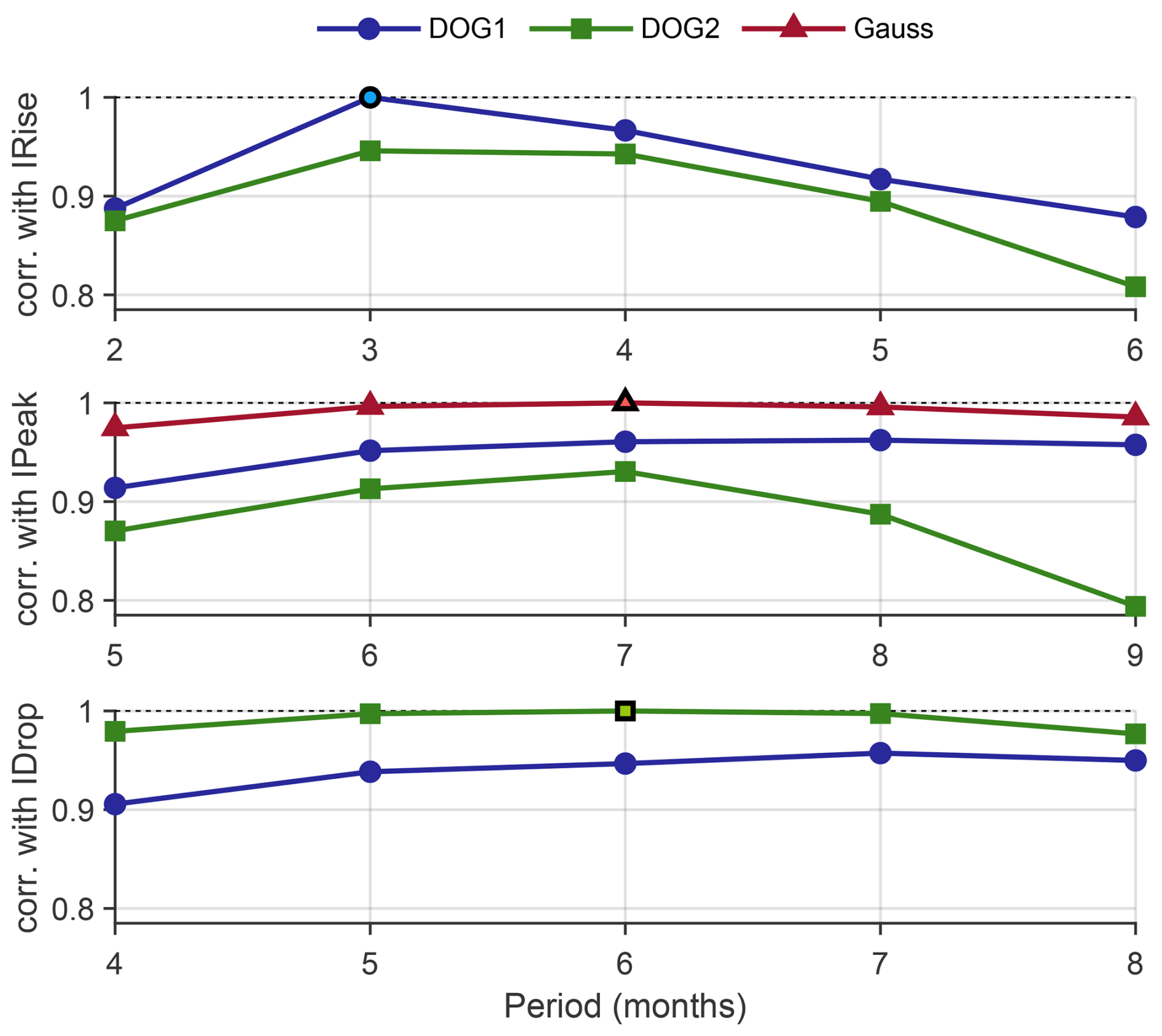
Figure 7 Sensitivity of IRise (top), IPeak (middle) and IDrop (bottom) to wavelet type and analysis period, expressed as correlation with the reference configuration. Wavelet types are indicated by marker shape and color: DOG2 (green squares), DOG1 (blue circles) and Gaussian function (red triangles). For each indicator, the reference configuration (IRise: DOG1, 3 months; IPeak: Gaussian, 7 months; IDrop: DOG2, 6 months) is highlighted by a lighter color and a black outline, corresponding to a correlation value of 1. The dashed horizontal line indicates perfect agreement.

The influence of wavelet selection was limited overall, as indicators computed using alternative wavelets showed consistently high correlations with the reference configuration. On average, changing the wavelet reduced correlations by 4.0 % for IRise, 4.2 % (DOG1) and 11.3 % (DOG2) for IPeak and 5.1 % for IDrop. Differences were smallest when wavelets shared similar shapes (e.g. Gaussian vs DOG1, DOG1 vs DOG2) and increased when moving toward more structurally distinct wavelets. For IPeak, deviations were most pronounced when using the DOG2 wavelet at periods longer than 7 months. At these scales, the temporal support of the wavelet approaches one year (about 360 d at an 8-month period), extending well beyond the current growing season and incorporating approx. 230–260 d preceding the start of carbon uptake. This extended support corresponds to increased contributions from the previous season.

Sensitivity to period selection differed among indicators. IPeak and IDrop showed limited sensitivity, with correlations relative to the reference configuration remaining above 0.975 across all tested periods and exceeding 0.996 within ±1 month of the reference period. In contrast, IRise was more sensitive to the analysis period, although correlations remained above 0.88 across all tested configurations. Lower correlations were observed at shorter periods (2 months), while correlations gradually decreased for longer periods. Additional tests at shorter periods (not shown) resulted in a marked drop in correlation (r=0.56 at 1 month), reflecting the inability of these time windows to capture the full spring rise.

Taken together, these results indicate that the proposed indicators are robust across a range of plausible parameter choices, while still requiring consistency between wavelet shape, temporal scale, and the targeted signal feature to avoid biased estimates.

3.3 Benchmarking

Comparison between indicators and reference values (Fig. 8) indicates strong overall agreement, all correlations being highly significant (p<0.001). In general, IPeak showed the strongest agreement between methods (r=0.96–0.98), with IRise following suit (r=0.88–0.96). IDrop comparisons presented more scatter (r=0.83–0.90), with large drops dominating the relationships. Years with relatively early GPP drops and strong late GPP drops tended to be more severely punished using the WAI and contributed strongly to the scatter. A notable example is year 2016 at FR-Hes: excluding this year increased the correlation to 0.95.

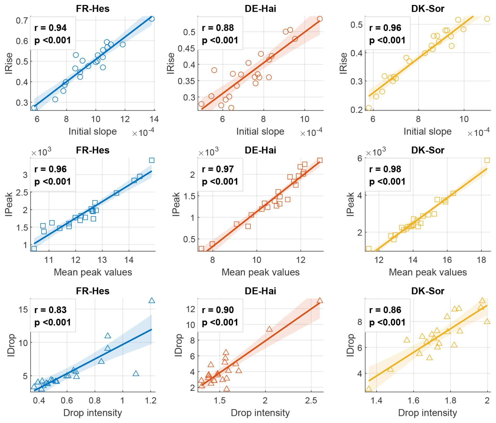
Figure 8 Benchmarking of the three GPP indicators: initial slope (IRise, top), peaking values (IPeak, middle) and mid-season drop intensity (IDrop, bottom). WAI-derived indicators (y-axis) are compared to corresponding values estimated using GPP time series (x-axis) for three forest sites (FR-Hes, DE-Hai and DK-Sor). Computation details are given in Sect. 2.4.3. Correlations and p-values are indicated for each relationship.

As for indicators, all phenological markers were significantly correlated to reference dates (p<0.001 for all correlations, see Fig. S7). When fixing the intercept to 0, slopes were all in range 0.99–1.01 for CUS and 1.04–1.06 for CUE. Estimated MSD on smoothed GPP was less correlated with WAI-derived metrics (r=0.69–0.80): slopes were highly different from 1 (in range 0.36–0.53) and significant shifts were found between metrics and reference dates (up to 40 d). Relationships at DK-Sor presented the lowest correlation with reference values for all metrics. At this site, early GPP increases and late GPP decreases were more progressive, which led to greater uncertainty in CUS and CUE.

3.4 Indicators

The mixed-effects models revealed substantial differences among sites for several indicators (Table 3).

Table 3 Estimated marginal means (EMMs) evaluated at a reference year (center point of each dataset) from linear mixed-effects model with Site, centered Year and Site × Year as fixed effects and a random intercept for Year. Grouping letters (referring to FR-Hes, DE-Hai and DK-Sor in order) denote homogenous groups from Holm-adjusted pairwise contrasts. Sites sharing a letter are not significantly different at α=0.05. The p-values are given for significant differences between sites and for Site × Year interactions. See Figs. 9 and 10 for time-varying differences. If Site × Year is significant, EMM and letters apply at reference year. Model results are detailed for each indicator (IRise, IPeak, IDrop) and phenological marker (CUS, MSD, CUE, CUL).

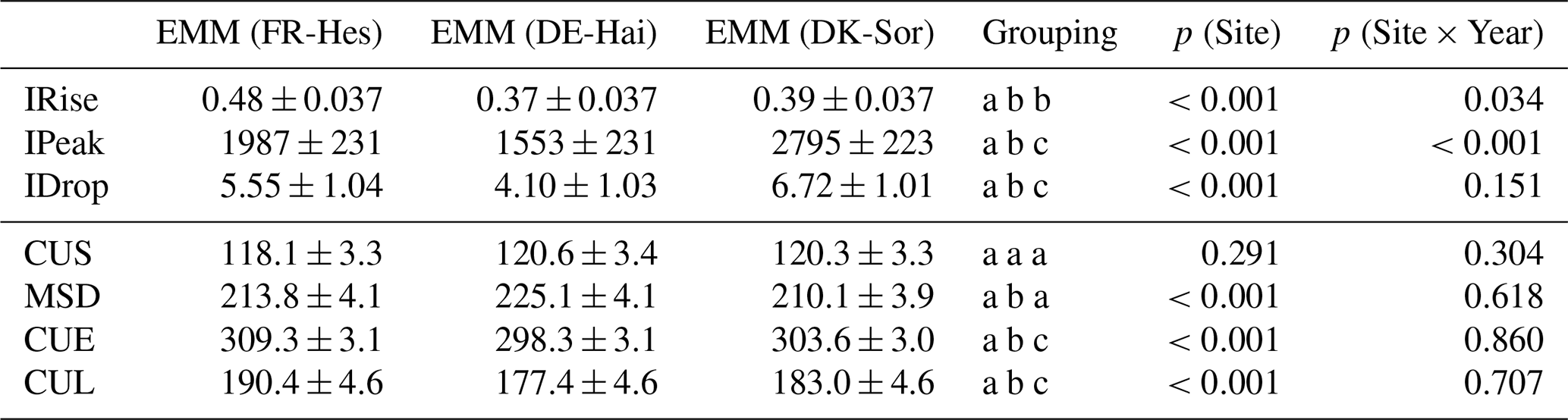
A significant Site × Year interaction was observed for IRise (p=0.034), indicating that differences among sites slightly evolve over time. This is consistent with the temporal trajectories of IRise, as only FR-Hes showed a significant decreasing trend (slope = −0.0065 yr⁻¹, p=0.032; Fig. 9). As a result, differences between FR-Hes and the other two sites tended to decrease over time. At the mean centered year, EMMs indicated higher IRise at FR-Hes (0.48 ± 0.037) compared to DK-Sor (0.39 ± 0.037) and DE-Hai (0.37 ± 0.037). Pairwise contrasts confirmed that FR-Hes exhibited significantly higher IRise than DE-Hai (difference: Δ= 0.11, p<0.001) and DK-Sor (Δ= 0.10, p<0.001), whereas no significant difference was detected between the latter two sites.

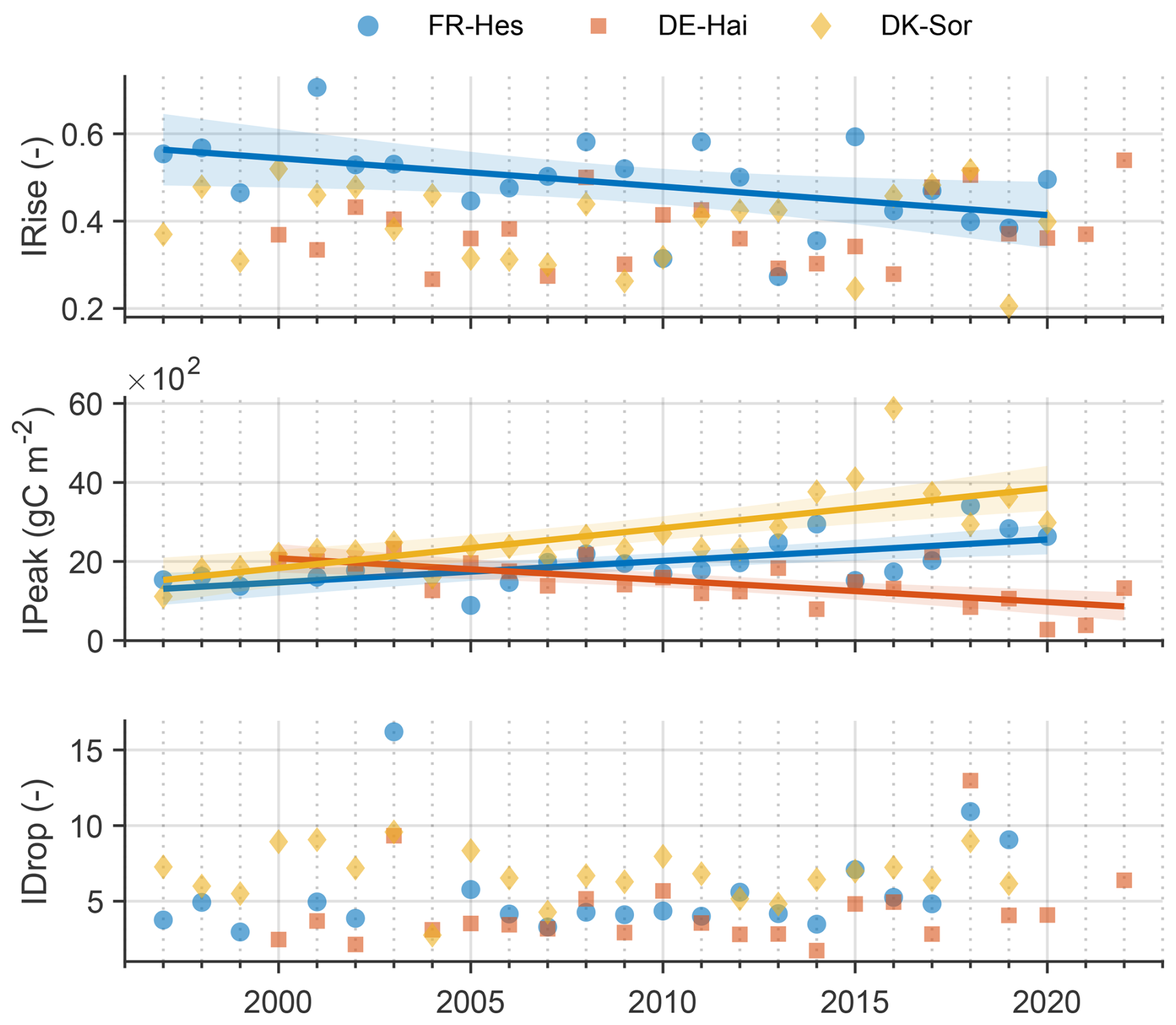
Figure 9 Temporal evolutions of the three indicators for the three forest sites (FR-Hes, DE-Hai, DK-Sor). Each panel corresponds to a different GPP indicator: initial slope (IRise, top), peaking values (IPeak, middle) and mid-season drop intensity (IDrop, bottom). Data points represent observed annual values for each indicator. When site-specific slopes were significant (p≤0.05), linear trends (solid line) alongside 95 % confidence intervals (shaded areas) are displayed. Note that indicator units are not directly interpretable, as they reflect wavelet-derived features rather than absolute physical quantities.

IPeak presented a highly significant Site × Year interaction (p<0.001), meaning that differences between sites were strongly time-dependent (as seen in Fig. 9). DK-Sor presented by far the fastest increase (slope = 101 gC m⁻² yr⁻¹, p<0.001) followed by FR-Hes (slope = 54.3 gC m⁻² yr⁻¹, p<0.001). On the other hand, IPeak values at DE-Hai decreased over years (slope = −55.4 gC m⁻² yr⁻¹, p<0.001). These dynamics lead to inter-site differences widening over time. Around year 2000, all sites presented similar IPeak values with DE-Hai being the highest by a small margin. By year 2020, GPP peaking values were significantly higher at DK-Sor, FR-Hes being intermediate and DE-Hai being the lowest (Fig. 9). At FR-Hes, LAI and IPeak were strongly correlated (r=0.85, p<0.001).

No significant Site × Year interaction was observed for IDrop (p=0.15). All three sites presented significantly different EMMs (Table 3). Values were highest at DK-Sor (6.72 ± 1.01), intermediate at FR-Hes (5.55 ± 1.04) and lowest at DE-Hai (4.10 ± 1.03), although DK-Sor presented no years with exceptional mid-season drop intensity contrary to the other two sites (Fig. 9). No significant temporal trend was detected for either site.

3.5 Phenology

Across all phenological markers, no significant Site × Year interaction was detected (Table 3), indicating that phenological differences among sites were consistent through time. Site effects can therefore be interpreted as overall differences in phenology, independent of temporal trends.

Pairwise comparisons of EMMs showed no significant differences in the CUS among sites. In contrast, the end of the carbon uptake period differed significantly between all three sites. DE-Hai exhibited the earliest CUE, followed by DK-Sor (Δ= 5.3 d, p=0.0048) and FR-Hes (Δ= 11.0 d, p<0.001). In consequence, CUL was significantly shorter at DE-Hai than at DK-Sor (Δ= 5.5 d, p=0.027) and at DK-Sor than at FR-Hes (Δ= 7.4 d, p=0.0032).

MSD occurred significantly later at DE-Hai than at both FR-Hes (Δ= 11.3 d, p<0.001) and DK-Sor (Δ= 15.0 d, p<0.001). The latter two sites did not differ significantly in mid-season drop timing.

A significant long-term trend was observed at FR-Hes (Fig. 10), where CUS advanced over time (slope = −0.43 d yr⁻¹, p=0.030). Temporal trends suggested a slight lengthening of CUL at DE-Hai (slope = 0.29 d yr⁻¹, p=0.45), DK-Sor (slope = 0.37 d yr⁻¹, p=0.28) and FR-Hes (slope = 0.73 d yr⁻¹, p=0.027), but the trend was significant only at the latter site. No significant temporal trends were detected for other sites and metrics. A noticeably late MSD was observed in 2014 at DE-Hai, reflecting atypical seasonal dynamics for that year.

Figure 10 Phenological markers for the three forest sites (FR-Hes, DE-Hai and DK-Sor). Years are displayed on the vertical axis (in reversed chronological order) and day of year (DOY) on the horizontal axis. Marker shape differentiates three phenological events: carbon uptake start (CUS, circle), mid-season drop (MSD, square) or carbon uptake end (CUE, triangle). Horizontal segments connect events within each year. Linear temporal trends are shown (in dashed lines) only when the regression slope is statistically significant (p≤0.05). Shaded bands represent 95 % confidence intervals around significant regression lines.

Correlations between indicators and between indicators and phenological markers were almost all non-significant. Interestingly, IRise showed a significant negative correlation with the mid-season drop date relative to CUS at FR-Hes ($r=-\mathrm{0.59}$, p=0.005) and at DE-Hai ($r=-\mathrm{0.65}$, p<0.001), suggesting that later GPP drops within the season are associated with lower spring GPP rise rates. A similar relationship was observed at DK-Sor ($r=-\mathrm{0.33}$, p=0.12), although non-significant. Nonetheless, this relationship becomes significant using the reference CUS ($r=-\mathrm{0.67}$, p<0.001) although relationships for other sites did not change, hinting to the difficulty of identifying phenological markers at DK-Sor using the GPP signal.

4 Discussion

4.1 Performance and robustness of indicators and phenological dates

The sensitivity analysis provides insight into the effect of methodological choices on the indicators. First, the limited impact of wavelet selection confirms that the method primarily depends on the ability of the wavelet to match the temporal structure of the targeted feature, in line with classical recommendations in wavelet analysis (e.g. Farge, 1992; Torrence and Compo, 1998). Wavelets with similar shapes produce comparable indicators, while more distinct wavelets introduce moderate deviations. This effect is particularly visible for IPeak, where deviations from a bell-shaped weighting lead to systematic differences, especially when using multi-lobed wavelets that integrate signal components outside the peak period. Second, the dependence on period selection reflects the nature of each indicator. IRise is the most sensitive because it represents a rate of change and therefore strongly depends on how the temporal window captures the growing phase. Periods that are too short fail to capture the full increase in GPP, while larger periods integrate more stable parts of the signal, leading to smoother but slightly dampened values. In contrast, IPeak and IDrop are inherently less sensitive to period. IPeak is centered on a stable maximum GPP and is therefore weakly affected by changes in period, especially when combined with smooth weighting functions (i.e. applying progressively lower weights farther from the peak). IDrop integrates information from both halves of the growing season, making it inherently less dependent on a specific temporal window. Taken together, these results emphasize that the method does not require precise parameter tuning, but rather a consistent alignment between wavelet shape, analysis scale, and the ecological process of interest. When this condition is satisfied, different configurations yield comparable indicators, supporting the robustness and transferability of the approach to other datasets.

Benchmarking against GPP “reference” values shows strong overall agreement, with IPeak and IRise exhibiting higher concordance than IDrop. This hierarchy is mechanistically intuitive: peak-season GPP is typically characterized by strong signal-to-noise ratio, while mid-season features (the drop) integrate multiple interacting stressors (e.g. vapor pressure deficit, soil moisture limitation, heat) and are therefore both more variable and more method-sensitive (Panwar et al., 2023; Rukh et al., 2023). Similarly, MSD is the most difficult phenological marker to recover robustly, with lower correlations and large potential shifts relative to smoothed GPP reference dates (up to 40 d). This is not surprising as mid-season “drop” is an emergent property of episodic stress, and thus it depends strongly on how the seasonal curve is smoothed and how “drop” is operationally defined.

More generally, the divergence between phenological markers was greater than for indicators. This is expected, as phenological dates derived from GPP are highly sensitive to smoothing and threshold choices (Panwar et al., 2023), whereas indicators integrate signal behavior over broader temporal windows and are therefore less sensitive to methodological choices. This increased sensitivity is further reflected in site-specific responses. The overall lower correlations of phenological markers at DK-Sor reflect the smoother spring and autumn transitions of GPP at this site. This is consistent with the stand's managed and relatively even-aged structure, as well as with the milder, maritime climate, which tends to produce more gradual seasonal transitions (Pilegaard and Ibrom, 2020).

4.2 Contrasting annual carbon balances across sites

Across the three temperate forest sites, the NEE is consistently negative (net sinks), but the magnitude and direction of temporal change differ markedly. The fact that interannual and long-term variations in NEE track GPP more strongly than Reco aligns with broader eddy-covariance evidence that productivity metrics tend to show stronger sensitivity to interannual variability and long-term change than ecosystem respiration (Baldocchi et al., 2018; Moreaux et al., 2020). Reco remains comparatively buffered because it is distributed across heterogeneous organ and microbial sources and constrained by substrate availability (Granier et al., 2008; Ngao et al., 2012).

The declining annual GPP at DE-Hai is consistent with mechanisms proposed for age- or size-related declines in forest production, where increasing tree height/size can introduce hydraulic limitations, reduce stomatal conductance, and depress photosynthesis, even if respiration does not increase proportionally (Drake et al., 2011). These mechanisms can operate at stand scale even when structural heterogeneity is high, as in old forests (Genet et al., 2010; Hesse et al., 2023). Conversely, increasing GPP at DK-Sor and FR-Hes is consistent with managed stand dynamics: thinning can sustain or enhance canopy light distribution and maintain higher assimilation capacity per unit leaf area, while stand development in younger/maturing forests can still be on the rising limb of productivity (Granier et al., 2008). Furthermore, frequent thinning enhances tree performance during drought by increasing soil water availability, reducing stand-level transpiration, and sustaining higher radial growth before, during, and after drought events (Sohn et al., 2016). These interpretations are consistent with long-term FR-Hes and DK-Sor records, which report increasing net CO₂ uptake and persistent flux-phenology relationships (Granier et al., 2008; Pilegaard et al., 2011).

4.3 Inter-site differences in indicators and phenology

The rate of increase in GPP (IRise), significantly higher at FR-Hes than at DE-Hai or DK-Sor, suggests a more rapid spring activation of photosynthesis in this relatively young beech-dominated stand. Nonetheless, IRise has significantly declined at FR-Hes over the study period. Concurrently, the CUS has advanced by approximately 0.43 d yr⁻¹, a rate slightly higher than previously reported for European beech stands (Schwartz et al., 2006; Skvareninova et al., 2024). These two trends are interconnected: an earlier CUS extends the time available to reach peak GPP, typically occurring near the summer solstice (median dates of 14, 21 and 22 June resp. for DK-Sor, DE-Hai and FR-Hes). Consequently, peak productivity is reached later in the GS, resulting in a slower overall GPP growth rate.

This advancement in budburst has been widely documented across beech stands in various climates and elevations (Bednářová et al., 2014; Fu et al., 2018; Prislan et al., 2019; Skvareninova et al., 2024; Stagakis et al., 2022). It is particularly pronounced in cooler climates and at higher altitudes, where beech phenology is more strongly regulated by temperature than photoperiod (Vitasse and Basler, 2013). In contrast, in warmer regions, photoperiod exerts a greater influence on spring phenology, offering a more stable seasonal cue than temperature, which is subject to local variability and extremes (Basler and Körner, 2012). Despite its mild climate and low elevation, the FR-Hes site exhibits a pronounced advancement in CUS (Prislan et al., 2019; Skvareninova et al., 2024; Vitasse and Basler, 2013), suggesting a strong temperature sensitivity in budburst timing, which contributes to the observed decline in IRise. The trend may be further amplified by the temperature dependency of bud development rates (Basler and Körner, 2014). However, the long-term trajectory of IRise remains uncertain, as beech at FR-Hes may adapt to warming by increasing its reliance on photoperiod to regulate ecodormancy release (Basler and Körner, 2012; Fu et al., 2015). This interpretation is consistent with the decreasing differences in IRise between FR-Hes and the other sites over time, suggesting a possible convergence in spring productivity dynamics. Additionally, pre-summer temperatures enhance IRise, which could partially offset the negative impact of earlier CUS on IRise. This compensatory effect may be moderated by two factors: (1) structural changes in the stand, as the FR-Hes beech stand presents an increased basal area and reduced tree density, which enhances LAI development (Bequet et al., 2011), and (2) shifts in the species composition, with a rising proportion of hornbeam and oak, species that exhibit respectively earlier and later leaf-out compared to beech (Zahnd et al., 2023). Nevertheless, no clear changes in IRise or CUS were observed following thinning, suggesting that the influence of species composition shifts remains limited.

IPeak shows both strong site differences and divergent temporal trajectories, with DK-Sor increasing most rapidly, FR-Hes increasing moderately, and DE-Hai decreasing. Explanations are most likely multifactorial as peak GPP integrates canopy capacity (leaf area, nitrogen status, light distribution), physiological constraints (stomatal regulation under VPD), and stand structure. For DE-Hai, the decline in IPeak aligns with expectations for an aging, unmanaged system where hydraulic limitations, competition, and structural senescence can reduce maximum canopy conductance and assimilation capacity (Drake et al., 2011). At FR-Hes, the forest experienced consistent biomass accumulation and canopy expansion, enhancing photon capture and CO₂ assimilation. IPeak therefore correlates strongly with LAI, a key driver of productivity (Le Dantec et al., 2000). In parallel, atmospheric CO₂ concentrations rose significantly at all sites. Elevated CO₂ concentrations enhance GPP by increasing substrate availability at Rubisco's catalytic site (Jiang et al., 2020; Stitt, 1991). Free-Air CO₂ Enrichment experiments and modelling studies have demonstrated that elevated CO₂ can also increase LAI by modifying crown architecture and promoting carbon allocation to shaded leaves (McCarthy et al., 2007; Norby and Zak, 2011). The observed correlation between CO₂ concentrations and LAI supports this hypothesis, although their relationship remains complex and is constrained by resource availability (Duursma et al., 2016). Furthermore, evidence of this effect is still scarce and most apparent in stands with low LAI (Norby and Zak, 2011).

IDrop shows no consistent temporal trend across sites. This variability is expected, as IDrop is primarily influenced by meteorological conditions during the growing season, particularly aerial and edaphic drought (Wankmüller et al., 2024). Beeches are known to show strong physiological sensitivity to drought and heat, including stomatal closure, reduced photosynthesis, and, during severe events, early senescence or canopy damage (Bréda et al., 2006; Leuschner, 2020). Large reductions in beech vitality and productivity have been reported during drought across Central Europe, with legacy effects and increased vulnerability to subsequent stressors (Rukh et al., 2023; Thomas et al., 2024). While drought frequency has increased in recent years, its intensity remains irregular, preventing the emergence of a monotonic trend.

Nonetheless, IDrop differs consistently among sites, indicating that the magnitude of mid-season reductions in photosynthesis represents a stable site-specific property. The unmanaged old-growth stand at DE-Hai displayed the lowest mid-season declines. This summer stability is consistent with features typical of unmanaged old-growth beech forests, i.e. deep and spatially heterogeneous rooting systems, multilayered canopies that buffer radiation and vapor pressure deficit, and a conservative water-use strategy that can mitigate short-term summer stress (Adhikari et al., 2025; Genet et al., 2010; Yu et al., 2022). In contrast, DK-Sor exhibited the highest IDrop values, reflecting stronger mid-season reductions in GPP. The stand's vertically concentrated canopy combined with high exposure to atmospheric conditions, likely amplifies summer constraints by producing a large proportion of leaves at the canopy top, where heat load and vapor pressure deficit are maximal (Bachofen et al., 2020; Pilegaard et al., 2003). Despite these larger reductions, DK-Sor also showed the lowest interannual variability in IDrop, suggesting that while mid-season declines are more pronounced, they occur with greater year-to-year consistency, reflecting the stability of its maritime climate (Chiesi et al., 2016; Pilegaard and Ibrom, 2020). FR-Hes showed intermediate values with large variability, consistent with its mixed management history, the more constrained hydrology of its luvisol/stagnic luvisol soils and its partially shifting species composition.

The absence of significant Site × Year interactions for all phenological markers implies that site differences in phenology have remained stable over time, despite ongoing climate change. CUS is remarkably similar among sites, suggesting that spring phenology is largely driven by regional climate rather than by stand structure or age. In contrast, CUE (and the overall CUL) differs significantly across sites, implying stronger influence of local stresses and stand properties. At DE-Hai, the earlier CUE suggests that late-season carbon assimilation is constrained, most likely by the forest's structural and physiological characteristics (Herbst et al., 2015). DE-Hai is an uneven-aged, old-growth stand where mature trees experience stronger hydraulic limitations and higher respiration costs (Curtis and Gough, 2018), making them more vulnerable to stress-induced declines in late-season productivity. In contrast, FR-Hes exhibits the latest CUE and the longest CUL. Although no direct evidence exists that younger stands systematically delay the end of the growing season, younger and fast-growing trees are known to show greater phenological plasticity and higher photosynthetic capacity per unit leaf area, which can translate into extended activity under favorable conditions (Vitasse, 2013). At this site, senescence timing has been shown to be a primary driver of interannual variability in CUL and GPP, with later senescence strongly associated with higher productivity (Granier et al., 2008). These features provide a plausible physiological basis for the prolonged carbon-active season observed at FR-Hes, even if autumn phenology drivers (including age effects) remain insufficiently quantified in current literature (Silvestro et al., 2025).

The negative correlation between IRise and the timing of the mid-season drop suggests a potential intra-seasonal trade-off: faster early-season development, driven by accelerated leaf expansion, leads to an earlier, though not necessarily more pronounced, decline in GPP. This pattern suggests a coupling between spring and autumn phenophases, where rapid spring development may trigger earlier senescence. Similar relationships have been observed across temperate and boreal forests (Zohner et al., 2023). They likely result from early-season warming, which accelerates leaf development but also promotes faster tissue maturation (Zani et al., 2020), hormonal changes (Chen et al., 2022) and downregulation of photosynthesis due to non-structural carbohydrates accumulation (Luo et al., 2024; Tian et al., 2024).

4.4 Interest of the WAI-based approach

The WAI follows directly from the mathematical structure of the CWT, yet its use and potential have, to our knowledge, not been described in scientific literature. This absence likely stems from historical perspectives: wavelet analysis has long been framed as a spectral tool derived from the FT (Debnath and Shah, 2015), and the intuitive “frequency-oriented” interpretation of Fourier coefficients was simply transferred to wavelets. As a result, alternative ways of interpreting individual wavelet coefficients have rarely been explored. In addition, applying WAI in practice requires selecting specific coefficients from the large number produced by the transform, and its interpretations depend on the shape of the chosen wavelet. These factors make WAI difficult to use as a standalone analysis tool. By embedding WAI within the structured 3-step workflow introduced in this study, coefficient selection becomes systematic, wavelet dependence becomes explicit and interpretable, and the method becomes reproducible and accessible to non-specialists. In this integrated form, WAI operates as a practical extension of wavelet analysis, enabling meaningful ecological interpretations of seasonal carbon-cycle patterns.

The WAI-based approach expands the information typically extracted from scalograms. Whereas classical wavelet analyses focus primarily on dominant patterns (i.e. local maxima in coefficient amplitude), examining peak distributions within period bands provides a systematic view of recurrent behaviors in the signal. This procedure highlights both regular seasonal features and irregularities, such as missing or isolated peaks, and greatly enlarges the set of wavelet coefficients that can be meaningfully interpreted. The WAI then links each selected coefficient to its contributing areas, enabling direct interpretation without relying on significance testing, although statistical tools can still assist in guiding exploration. Although different wavelets may emphasize different structures, the DOG2 wavelet generally offers a robust starting point for ecological applications due to its stability in detecting peaks and trend discontinuities.

This broader interpretative capacity makes it possible to construct various indicators that closely match specific signal features. While some metrics could theoretically be approximated by simpler measures (e.g. numerical slopes for IRise), such substitutions lack the versatility and sensitivity of the WAI approach. The dates identified from period-band peaks determine the temporal windows used for indicator calculation, removing the need to define external positioning criteria. The method also avoids explicit signal manipulation: no smoothing, thresholds, or curve fitting are required. This is particularly valuable because choices in smoothing or thresholding can shift phenological transition estimates by weeks, with uncertainties especially large near transitional periods where the GPP signal is weakest or most complex (Panwar et al., 2023). These considerations are central for defining the MSD, which is often not a discrete event but a consequence of intra-seasonal variability in ecosystem conditions. This characteristic is illustrated by years such as 2014 at DE-Hai, where an atypical early-season reduction in GPP resulted in delayed MSD positioning, highlighting the sensitivity of this metric to intra-seasonal variability. As a result, MSD should be interpreted with caution at the annual scale and is more robust when used to assess interannual patterns (e.g. median timing or trends), or to characterize years with pronounced mid-season declines (e.g. drought events).

Finally, WAI offers practical advantages for working with real-world ecological data. Like Fourier-based approaches, CWT assumes continuous, regularly spaced inputs, which is rarely met in environmental records. By targeting specific coefficients, the WAI limits this requirement to the wavelet support, allowing small gaps within that interval to be handled using local gap-filling without altering the broader analysis. Nonetheless, indicator stability still depends on data quality, and large gaps or low-quality periods can influence results. Within these constraints, however, the WAI-based workflow provides a robust, reproducible, and flexible way to extract ecologically meaningful information from complex time-series.

4.5 Perspectives in ecology

A key strength of the WAI-based 3-step approach is its ability to detect recurring patterns even when the spacing between events is irregular. Because the method operates on the distribution and structure of wavelet coefficients, it can identify repeated behaviors regardless of their periodicity or strength. This property is particularly valuable for ecological applications in which seasonal dynamics are weak, episodic or highly variable across years. Tropical ecosystems, for instance, often exhibit aseasonal or event-driven productivity pulses, or shorter and less predictable growing seasons compared to temperate forests (Reich, 1995). While Fourier-based analyses have been used to describe such flexible cyclicity (Bush et al., 2017), they do not provide temporal localization of events. By contrast, the WAI approach naturally accommodates these systems, allowing both the timing and the strength of recurrent features to be compared across periods. More broadly, similar characteristics are found in other land-cover types such as grasslands with multiple growing cycles or disturbance-driven systems (e.g. drought- or fire-affected ecosystems). For ecosystems with relatively well-defined and recurrent seasonal cycles, transferability is expected to be direct, as similar signal structures can be targeted. Conversely, systems characterized by weak, irregular or event-driven dynamics require a more exploratory application, with greater reliance on WAI visualization to identify relevant features and less systematic definition of indicators.

Beyond identifying patterns, the indicator framework enables direct comparison of signals through a small, interpretable set of metrics. Indicators summarize the behavior of specific signal features, allowing comparisons among sites, ecosystems or experimental treatments without relying on full time-series inspection. This is particularly valuable for multi-site analyses, where similar processes may express differently depending on local constraints. The approach also provides a practical tool for model evaluation: discrepancies between observed and simulated indicators highlight which aspects of ecosystem dynamics are well or poorly represented in the model.

Linking indicators to environmental drivers offers another promising direction. Long-term ecological studies often rely on broad annual metrics, such as sums (Baldocchi et al., 2018) or anomalies (Aubinet et al., 2018), or multiscale methods, such as time-series decomposition (Wu et al., 2012), random forests (Moreaux et al., 2020), or wavelet decomposition (Sturtevant et al., 2016). Because indicators isolate specific signal features, their correlations with drivers provide a complementary lens, by revealing localized and process-specific influences that are not captured by aggregated metrics. This can enhance our understanding of ecosystem-atmosphere interactions, stress responses, and population or community dynamics, and ultimately improve model parameterization. Exploring these relationships is the focus of the companion paper (second part of this study), which examines how indicator-driver linkages elucidate the mechanisms underlying interannual GPP variability.

The WAI-based date selection approach also opens new possibilities for phenological research. Metrics such as canopy development, senescence timing or growing-season boundaries are typically derived from smoothed vegetation indices and threshold- or derivative-based methods (Caparros-Santiago et al., 2021). Our method avoids assumptions about curve shape and does not require smoothing, as dates arise directly from discontinuity detection in the signal. This ensures period-specific adaptation and improves robustness when dealing with complex or noisy seasonal transitions. However, performance still depends on data quality and on selecting an appropriate wavelet, since inadequate choices can obscure subtle or short-lived events. WAI visualization offers a practical way to guide these decisions. Because the method relies on the detection of localized peaks in the wavelet domain, it reduces the number of arbitrary methodological choices compared to threshold-based approaches. In combination with independent phenological observations, this feature-based selection provides a flexible yet robust framework for identifying key transitions in ecosystem dynamics.

Finally, the WAI framework could be extended to bivariate wavelet tools such as the cross-wavelet transform or wavelet coherence, which examine relationships between variables (Cazelles et al., 2008). These methods are powerful but limited when analyzing delayed effects, because their usable lag range is constrained by the wavelet support, shape and complex/real nature. Ecological studies give increasing attention to delayed effects, particularly in recent years (Aubinet et al., 2018). If driver-response lags are expected, the indicator-comparison framework provides greater flexibility, as lags can be adjusted manually within the limits of the dataset.

While these perspectives highlight the versatility of the approach, its application remains subject to several methodological constraints that should be considered.

First, the approach relies on the assumption that the wavelet shape and the selected scale appropriately reflect the temporal structure of the targeted signal feature. Although the sensitivity analysis shows that indicators are robust across a range of plausible configurations, inappropriate choices may still lead to biased estimates, particularly when the temporal extent of the process is not well constrained.

Second, while the method avoids explicit smoothing of the signal, it remains sensitive to data quality. Noise, gaps, or residual biases in eddy covariance data can affect the computation of wavelet coefficients, especially at short periods where the number of detected features increases.

Third, the interpretation of indicators depends on the assumption that seasonal features are sufficiently well defined in the signal. In ecosystems with weak or highly irregular seasonality, or where multiple overlapping processes occur, the identification of consistent features may become more uncertain.

Finally, although the framework is designed to be transferable, its application to other ecosystems requires careful adaptation of wavelet selection and analysis scales to the specific temporal dynamics of the system. In this respect, visual inspection and preliminary sensitivity analysis remain essential steps of the workflow.

5 Conclusions

This paper introduces a wavelet-based framework that systematically identifies recurrent seasonal events in ecosystem carbon-flux time series. By using the full structure of wavelet coefficients rather than a restricted set of significant power regions, the approach provides a flexible and scale-aware foundation for characterizing seasonal dynamics in gross primary productivity. The WAI method enabled the extraction of consistent carbon-uptake phenological markers while the three structural indicators (IRise, IPeak and IDrop) offered complementary information about the timing, magnitude and internal shape of the seasonal GPP cycle. Benchmarking against smoothed-GPP references confirmed the robustness of these indicators, especially for spring rise and peak productivity, while clarifying the expected uncertainty in mid-season metrics.

Applied to long-term eddy-covariance records from three contrasting European beech-dominated forests, the framework revealed clear and ecologically meaningful differences in seasonal structure and long-term carbon-sink trajectories. The unmanaged old-growth forest exhibited declining peak productivity and a shortening effective carbon-uptake period, while the two managed stands showed sustained or increasing productivity, highlighting the combined influence of forest age, management and climate. Across sites, the indicators exposed consistent seasonal contrasts (such as rapid spring activation, variable mid-season resilience, and site-specific end-of-season timing) and uncovered an intra-seasonal trade-off linking strong spring growth to earlier mid-season declines.

Together, these findings demonstrate that the proposed wavelet-based approach provides a powerful and broadly applicable tool for extracting ecological information from noisy, non-stationary signals. It opens new avenues for understanding how seasonal processes scale to long-term carbon-sink dynamics, and how forest responses to climate and management evolve across decades. As long-term flux networks continue to expand, such tools will be increasingly valuable for diagnosing ecosystem change and improving predictions of forest carbon dynamics under future climate conditions.