Quantifying the impact of groundwater fauna and temperature on the ecosystem service of microbial carbon degradation; a proof-of-principle approach

Groundwater ecosystems fulfil functions that humankind relies upon, e.g. for sustainable drinking water production. Quantification of these services is lacking so far. Thus, it is not possible to predict scenarios (e.g. future climates). Based on data from a comprehensive groundwater ecosystem study comprising four zones of varying land use and groundwater/surface water exchange, we parameterized a quantitative dynamic food web model (recharged organic carbon, microorganisms using the biodegradable fraction of this carbon, and fauna grazing on the microorganisms), in a proof-of-principle approach. With the model satisfactorily reflecting the field data, we calculated five further scenarios, three of which without fauna (mortality e.g. due to contamination, sudden peaks of temperature etc.). Two of the “fauna” and two of the “no fauna” scenarios were run with temperature elevated by 1.5 and 3 °C, respectively. The ecosystem service of carbon degradation was expressed as the difference in carbon concentration between the beginning of the simulation and the end of the simulation. In most scenarios, remaining carbon increased over time. The remaining carbon in some scenarios was up to 6.6 times as high in the “no fauna” scenarios compared to the reference case. Fauna was thus shown to fulfil a service by promoting microbial carbon degradation that may be substantial. This model set up can serve to test other cases of varying physical and chemical variations and disturbances.

1 Introduction

Ecosystems deliver services that humankind depends upon (Daily et al., 2010). On the surface of the Earth, such services include pollination (Landis, 2017), production of nutrition (Leclère et al., 2020), transformation and decomposition of dead biomass (Blouin et al., 2013), recreational opportunities (Eigenbrod, 2016), and water purification (Mori et al., 2025), which is a prerequisite for drinking water production (Tockner, 2021).

Groundwater, i.e. sensu lato the water beneath the surface (Winter et al., 2003), is also an ecosystem (e.g. Malard et al., 2023a; Directive (EU) 2026/805). Microorganisms are found almost everywhere in groundwater, depending on different conditions (e.g. Griebler and Lueders, 2008). They produce biomass (e.g. Magnabosco et al., 2018) which may be the food source for other organisms such as protozoa and fauna (Mermillod-Blondin et al., 2025). Groundwater ecosystems, although still often ignored, deliver, among others, the ecosystem services reworking of sediments (Stumpp and Hose, 2013) which limits colmation, i.e. the clogging of sediments (Descloux et al., 201), and water purification (Avramov et al., 2010; Mammola et al., 2026). When undisturbed, this purification results often in drinking water quality (Avramov et al., 2010) through e.g. pathogenic microorganisms being removed (Tufenkji et al., 2004), pollutants being biologically degraded (Meckenstock et al., 2015), and naturally occurring carbon being transformed (Marxsen, 1981; Herrmann and Taubert, 2022). Such purification takes time and is only possible in groundwater flowing slowly (probably maximum 1 m d⁻¹) through sediments or fractures with small pore sizes. In this contribution, we focus on such relatively deep and relatively old porous groundwater, i.e. not the subsurface water in continuous exchange with the surface and the atmosphere.

The entire food web in groundwater (Malard et al., 2023b) may be involved in groundwater purification through its processing of carbon. The groundwater food web is often truncated (Gibert and Deharveng, 2002), but may encompass several trophic levels (Ercoli et al., 2019; Malard et al., 2023b), depending on the respective environmental conditions. Some groundwater food webs are qualitatively well described, in terms of e.g. “who eats whom” (Bradford, 2009; Bradford et al., 2010; Ercoli et al., 2019; Francois et al., 2016; Leijs et al., 2015). Quantitative evaluations are scarcer (but see e.g. Foulquier et al., 2011; Mermillod-Blondin et al., 2025). However, this function of purification or self-cleaning in groundwater, i.e. degrading carbon compounds (Becher et al., 2022) to ultimately the gases CO₂ or CH₄, is probably most relevant to humans. These functions are one prerequisite for sustainable drinking water production, which is one of the 17 goals (goal 6) of the 2030 Agenda for Sustainable Development (United Nations General Assembly, 2017). Where groundwater communities decline or vanish, this may lead to deteriorating groundwater health (Koch et al., 2024a), compromising an aquifer's ecosystem and its function. The new directive (EU) 2026/805 demands in recital 20 “to reduce the level of purification treatment required in the production of water”. This is only possible if humankind makes sure that groundwater remains at or is developed towards a productivity of the whole food web that reduces organic matter most efficiently.

Heterotrophs are the main players in degrading organic matter (Benner, 2011) and thus purifying the groundwater (Avramov et al., 2010). Primary production in the case of groundwater, where light is lacking, is only possible in the form of chemolithoautotrophy. While chemolithoautotrophy is more prevalent than previously thought (Kellermann, 2008), heterotrophy, i.e. using organic resources that enter the groundwater ecosystem with groundwater recharge, will dominate in most places (Herrmann et al., 2015). Where heterotrophic degradation of imported organic material yields sufficient energy, a further level of the food web may be supported, i.e. grazers consuming producers, which in the case of groundwater is the basal microbial community including both autotrophs and heterotrophs sustained by imported organic matter. When and where even the producer biomass becomes substantial, a further level may be added, i.e. predators preying on grazers and deposit feeders (Ercoli et al., 2019; Saccò et al., 2019). In the following, we will include deposit feeders in the notion “grazers”. There are few taxa with just one feeding mode – most groundwater fauna will be grazing for at least part of their life cycle (Hose et al., 2022). It is well-known that grazing either reduces (Kota et al., 1999) or advances (Mattison et al., 2005) bacterial biodegradation of contaminants. Thus, adding levels to the food web might increase or it might compromise remediation and attenuation, i.e. oxidizing or reducing organic carbon to CO₂ or CH₄, respectively, which may leave the groundwater system as gases. It can be assumed that the biomass and energy in a respective level reduces to 10 % of the underlying level's biomass and energy (Lindeman, 1942; Odum, 1957). The loss is due to respiration which occurs due to mobility, reproduction, hunting etc. (Kozłowski, 1992), and in a full budget, would result in outgassing of CO₂ (or CH₄ in an anoxic system; Herrmann and Taubert, 2022; Nydahl et al., 2020) from the respective compartment, because of respiration (Moinet et al., 2023). Under which circumstances, both on temporal and spatial (Saccò et al., 2024) scales, which complexity of the food web emerges, is still largely unknown and has thus been near-impossible to parameterize.

While structuring food webs with just producers, grazers, and predators is grossly simplifying, this pattern has successfully been used e.g. in conceptualizing biomanipulation where e.g. predatory, piscivorous fish are added to a water body which harbours producing algae, grazing zooplankton and zooplankton-consuming planktivorous fish (Carpenter et al., 1985; Vrba et al., 2024). In such systems, commonly, the planktivorous fish reduce the zooplankton so that the algae are not grazed upon, may grow to harmful algal blooms and thus, deteriorate the water quality (Dadi et al., 2023). By adding piscivorous fish, the planktivorous fish are reduced, thus, more zooplankton remains which grazes more efficiently the algal blooms (Triest et al., 2016). Adding piscivorous fish is thus one measure for improving water quality. Is such management possible in groundwater as well? Or, vice versa, will the loss of grazing fauna result in lower water quality?

In Germany, depending on the region and meteorological situations, ca. 50 % of drinking water is produced from groundwater. In drinking water production, it is advantageous to have raw water with low organic substances (Moona et al., 2021) so that little respiration (which would reduce the dissolved oxygen) takes place in the pipes on the way to the customers (Kekes et al., 2023). Where dissolved oxygen is low or lacking, respiration of organic substances may lead to CH₄ which may be harmful to organisms and might thus limit degradation further. Anoxic conditions, resulting from respiration of excessive carbon sources, may lead to reduction of substances, and thus, dissolution of compounds which are bound in macro molecules at oxic conditions. E.g. aluminium, iron, etc. may become soluble at anoxic conditions (Dadi et al., 2023), and may be toxic to organisms. Thus, high raw water quality, with low levels of carbon, begins in the aquifers with a community of active organisms, degrading the recharged carbon and ensuring high oxic state throughout the drinking water production (Schubert, 2002; Fowler and Smets, 2017).

In addition to reduced conditions leading to undesired dissolved compounds, recently, brownification has become increasingly a problem (de Wit et al., 2016). One source of high molar mass organic compounds colouring the water yellow or brown is forest die back (Kopáček et al., 2023). The combination of dry summers stressing trees, and bark beetles making use of higher temperatures to produce more offspring than at colder climates (Seidl and Rammer, 2017) have led to expansive forest die back, e.g. in the Hercynian mountains (Musolff et al., 2024) in Germany and the Bavarian and Šumava mountains at the German-Czech boundary (Schmidt et al., 2024a). This sudden increase of tree biomass is broken down to organic dissolved compounds recharging into soil and groundwater many of which are undesired in drinking water production.

But higher temperatures have more, and more direct, effects than just favouring bark beetle generation times and dry summers. Dissolved oxygen solubility in water decreases with increasing temperatures (Retter et al., 2020), and brownification is believed to be exacerbated by increased temperatures (Blanchet et al., 2022). For these, and further reasons, the temperature regime in a groundwater body is important when evaluating the current and potential future state of an aquifer. Globally, air temperature has increased by 1.5 °C compared to pre-industrial times in 2025 (Bevacqua et al., 2025). The temperature increase in groundwater is delayed (Benz et al., 2017) and depends strongly on soil and geological properties and hydrological processes (Rau et al., 2015), but has, e.g. in Austria, reached approximately 0.4 ± 0.5 K per 10 years, meaning that an increase of 1.5 °C might be observable within 40 years. Benz et al. (2024) predicted that between 2000 and 2099, groundwater will warm on average by 2.1 °C, under a medium emission pathway. It is thus important to estimate which effect these temperature increases will have on the groundwater ecosystem.

On top of increased carbon input and higher likelihood for reduced conditions, increasing temperatures also impact groundwater organisms directly. E.g., increasing temperatures were related to increased microbial biomass in a temperature plume in Southern Germany, with the microbial community changing qualitatively (Brielmann et al., 2009).

Organisms adapted to the surface and its daily influence, i.e. stygoxene and stygophile metazoa, called fauna from here on, will cope with surface temperature ranges, while fauna adapted to the groundwater without daily influence, i.e. usually at least meters and months away from surface influence, are usually not well adapted to temperatures deviating from groundwater temperatures. In a meta-analysis, Vaccarelli et al. (2023) showed that all physiological response variables tested (stress response, mortality, and metabolism) exhibited statistically significant effects from climate change. A temperature of 20.2 °C was found to be lethal for half of the tested individuals of the groundwater crustacean niphargid Niphargus inopinatus after 25 d (Brielmann et al., 2011). However, the groundwater taxon Niphargus longicaudatus, with a wide geographic distribution, showed a wide temperature range in laboratory experiments (Di Cicco et al., 2023).

A groundwater niphargid and asellid differed in the temperature range they tolerated, with the niphargid covering a wider range (Brielmann et al., 2011). While we do not know whether these two species were among those present in the study area of this contribution (introduced below), until we have better data, we assumed the parameters from Brielmann et al. (2011) to be representative enough for a modelling study. Spengler and Hahn (2018) identified a threshold value for middle European groundwater systems of 13 °C above which fauna community changed drastically in composition. Avramov et al. (2013) and Brielmann et al. (2011) performed tests analogous to toxicity tests and extrapolated lethal temperatures for various durations of exposure. Like for the favoured temperature ranges, niphargids survived longer at higher temperatures than asellids. The lethal temperatures from these experiments can be used to parameterize fauna temperature-related mortality in models. Effects of temperature on the sublethal level, e.g. dissolved oxygen consumption, have also been quantified (Di Lorenzo and Galassi, 2017) and should be included in future models – here, we concentrate on the lethal temperature effect on fauna only.

In extreme cases, in summary, a temperature increase of a few °C may be lethal to groundwater fauna (Vaccarelli et al., 2023). Groundwater fauna is thus threatened from extinction (Noethen et al., 2024), like, globally, a quarter of freshwater fauna (Sayer et al., 2025). In contrast to climate opportunists following along the preferred temperature range (Dormann et al., 2018), groundwater fauna's expansion or retreat is limited by the aquifers' physical boundaries (Iannella et al., 2020). For the same reason, any faunal community not coping with increased temperatures will probably not be replaced by a higher-temperature-adapted community.

A consequence of the microbial community changing qualitatively in a temperature plume such as observed by Brielmann et al. (2009) may be a change in microbial ecosystem function. This has so far rarely been characterized, one exception being Brielmann et al. (2011). The microbial community is the main food source for groundwater fauna. On the regional and landscape scale, clear correlations between faunal associations and temperature have so far usually been missing, which is mostly due to the number of influencing and interacting factors (dissolved oxygen, varied toxicants, land use and development over time for all such factors) in relation to the often low numbers of samples (Koch et al., 2021).

The impact of temperature on organisms has implications on ecosystem services. Avramov et al. (2013) demonstrated the response of crustacea to increasing temperatures. Increased stress in the sense of disturbance, particularly when it is of the ramp or press type (Lake, 2000), which continuously increasing temperature presents, might lead to decreased fitness, and thus, decreased ecological functions (Holmstrup et al., 2018; Taborsky et al., 2022). Where temperature is so high that fauna and thus its ecosystem function are compromised or even lacking, any effect of microorganisms being more active at higher temperatures, and thus degrading more carbon, may be (more than) compensated by the lack of grazing and thus rejuvenating microbial growth (Mattison et al., 2005).

To this date, no quantitative evaluation of ecosystem services in groundwater and their susceptibility to temperature existed. However, we urgently need to quantify the impacts of temperature on groundwater ecosystem services since we may have to future-proof drinking water production if groundwater ecosystems change their functionality due to increasing temperatures, changing climates, and land uses (Schmidt et al., 2024b).

Since it is hard to derive the relevant data sets on the required temporal and spatial resolution, while controlling for different environmental settings globally, one way to approach answers to these questions are models. Here, we present a model, as a proof-of-principle approach, based on data from one of the most comprehensive data sets on a groundwater ecosystem, in the River Fulda floodplain (Husmann and Marxsen, 1988; Marxsen et al., 2021). While many groundwater taxa are ubiquitous, neighbouring aquifer zones may differ markedly in fauna taxa composition (Di Lorenzo et al., 2025a), and so it was for the River Fulda data set, although of small size (3 km²; Marxsen et al., 2021). The River Fulda data set thus enables us to study reactions to scenarios of increased temperatures and/or setting fauna biomass to 0 as if after a calamity, in different environmental exchange conditions, under the same climate. The data set allowed to check whether the developed model represented a range of measured field conditions. Fauna being absent might also be a consequence of climate change, since, as described, fauna does not survive well elevated temperatures. Admittedly, the data from the River Fulda floodplain within the narrow zone of river-near aquifers, might not be representative for many aquifers. However, we lack data that are representative for those aquifers relevant to our drinking water resources, and thus, we decided to take the data from one of the most comprehensive studies and made further assumptions relating to more secluded aquifers with a low range in temperatures and low adaptation of fauna to higher and lower temperatures.

The hypotheses in this proof-of-principle approach were: (1) Without fauna, a groundwater ecosystem shows lower carbon degradation, thus, higher remaining organic carbon. (2) An increase in temperature by 1.5 or 3 °C leads to an increase in microbial degradation, and thus, lower remaining organic carbon. (3) Fauna is compromised more by increasing temperatures, than microorganisms profit from a temperature increase; thus, a scenario of modelling fauna at a temperatures increased by 1.5 °C and more so at 3 °C will show decreased degradation of organic carbon, leading to higher organic carbon remaining than in the reference scenario with fauna at current temperature.

2 Study area and methods

The data that the proof-of-principle approach modelling was based on, were taken from a field study in the Johannisaue, River Fulda floodplain, described e.g. in Husmann and Marxsen (1988) and Marxsen et al. (2021). This study is to this date one of the most comprehensive (chemical and physical conditions, prokaryotes and fauna; microbial growth rate measurements) and longest-running studies (measurements between 1978 and 1984), including dividing prokaryote cells into size fractions allowing detailed biomass distributions. The size of the studied region was 3 km² (Marxsen et al., 2021), with the distances among wells ranging from 100 to 2028 m from each other (Table S1 in the Supplement).

Marxsen et al. (2021) had performed a k-means cluster analysis on the physical and chemical properties of the River Fulda data set (locality: Johannisaue), assuming four groups. One group combined wells near the river Fulda and in intense exchange with the river (“R”; Fig. 1), one group covered wells that were characterized by a plume of a carbon source from the near-by village (“P”), one group was characterized by agriculture with elevated nitrogen and phosphorus concentrations (“A”), and the fourth group represented wells of a mixing zone being situated in-between the other three zones and combining characteristics of all zones (“M”; Fig. 1). These groups are used here for different exchange situations at the same climate. The data set allowed checking whether the developed model represented a range of measured field conditions.

Once satisfied with the model, it is possible to change parameters and/or exclude fauna biomass to run scenarios representing warmer climates, and comparing ecosystem functions (here: degradation of organic carbon) when fauna is present versus absent. Fauna being absent might also be a consequence of climate change (see above). Admittedly, the data from the Johannisaue within the narrow zone of river-near aquifers, might not be representative for many aquifers. However, we lack data that are representative for those aquifers relevant to our drinking water resources, and thus, we decided to take the data from one of the most comprehensive studies and made further assumptions relating to more secluded aquifers with a low range in temperatures and low adaptation of fauna to higher and lower temperatures.

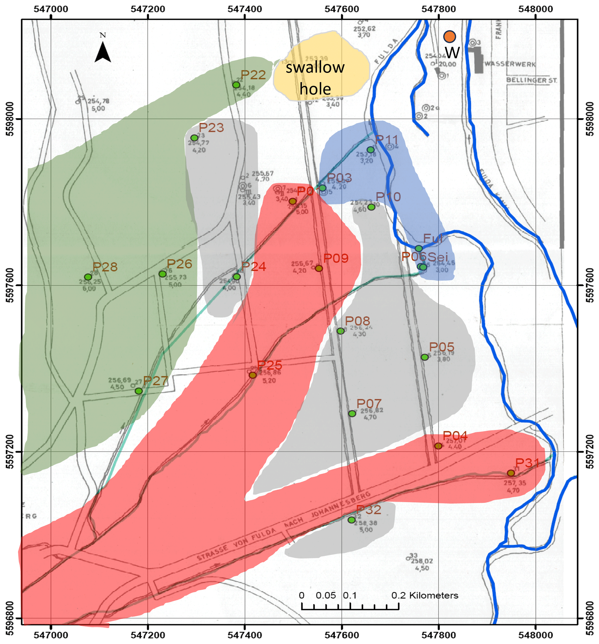
Figure 1 Map of the study area near Fulda, with the four groups of wells derived in Marxsen et al. (2021) colour-coded. Blue: river-near, abbreviated as “R”, grey: mixing zone (“M”), red: plume (“P”), and green: agricultural area (“A”). W: weather station Fulda Horas, DWD 1526. Changed after Marxsen et al. (2021). Coordinate system: ETRS 1989, UTM Zone 32N.

Groundwater temperature was only measured at the time of sampling in the wells in the river Fulda floodplain, i.e. at the maximum monthly. Therefore, we took the daily temperatures from the DWD (German weather service) station Fulda Horas (1526, 255.00 m above sea level (m a.s.l.); geographical latitude 50.5335; longitude 9.6750; on the east shore of the river at the north of the investigated area; “W” in Fig. 1). From the relationship of the minima and maxima of the in situ groundwater temperatures, compared to the minima and maxima of the Fulda Horas air temperature, we derived daily groundwater temperatures separately for the four groups of wells (Sect. S2 with Fig. S1). These were the basis for the scenario runs where temperature was one variable influencing maximum microbial growth rate and microbial half saturation concentration (refer to Sect. S5 in the Supplement for further explanations). We used the precipitation data from the same meteorological station 1526: Fulda Horas for estimating recharge (Sect. S3 in the Supplement). We then modelled carbon import into groundwater by multiplying the respective daily recharge volume from precipitation with an average carbon concentration. All carbon sources, and all organism compartments, were transformed to mol COD, i.e. chemical oxygen demand, to allow directly comparing compartments. See Sect. S4 in the Supplement for these calculations.

We assumed here that detritus would largely stay in the catchment. We further assumed that BOC would be the more influential factor for food webs and drinking water production, as e.g. in Vogt et al. (2023), and thus, we focussed on BOC and its pathway in the following.

For modelling microbial and faunal growth, we chose hybrid Monod/Verhulst models (Schlogelhofer et al., 2021), combining resource-dependent growth with the limiting factor of a carrying capacity. For microbial growth, the equation reads

$$\begin{array}{}\text{(1)}& \begin{array}{rl}{\displaystyle \frac{d_{{\mathrm{MO}}_{\mathrm{het}}}}{\mathrm{d}t}}& ={\mathit{\mu }}_{max,\mathrm{MO}\mathit{\_}\mathrm{het}}{c}_{{\mathrm{MO}}_{\mathrm{het}}}\\ (\mathrm{1}& -{\displaystyle \frac{c_{{\mathrm{MO}}_{\mathrm{het}}}}{K_{{\mathrm{MO}}_{\mathrm{het}}}}}\left)\right({\displaystyle \frac{c_{\mathrm{BOC}}}{K_{\mathrm{S},\mathrm{BOC}}+c_{\mathrm{BOC}}}})\end{array}\end{array}$$

where c_BOC is the concentration of biodegradable organic carbon (BOC; see below), c_{MO_het} is the concentration of heterotrophic microorganisms, μ_{max,MO_het} the maximum growth rate of heterotrophic microorganisms, K_{MO_het} the carrying capacity, and K_S,BOC the half saturation concentration (Schlogelhofer et al., 2021). We derived growth rate and carrying capacity from the maximum biomass (dry mass) measured in the wells and their temperature dependence (Sects. S5–S7 in the Supplement). Modelled biomasses unlimited by something like a carrying capacity tend to increase exponentially because natural limiting processes such as heterogeneity of the environment are not incorporated in the model. The equation for faunal grazing on microorganisms was built accordingly. For fauna, the model was implemented with c_{MO_het} instead of c_BOC, c_fauna instead of c_{MO_het}, μ_max,fauna instead of μ_{max,MO_het}, K_fauna instead of K_{MO_het} for the carrying capacity, and K_{S,MO_het} instead of K_S,BOC for the half saturation concentration.

With the paradigm “Everything is everywhere but the environment selects” (Baas Becking, 1934) still holding (de Wit and Bouvier, 2006), microorganisms can be assumed to change in composition when environmental conditions change. The functionality largely remains the same, due to functional redundancy (Taubert et al., 2019). For microorganisms, there is no mortality in the stricter sense. Instead, maximum growth rate and carrying capacity are parameters usually describing limited growth quite well. Since most bioreactions are most efficient at temperatures between 25 and 35 °C (Kong et al., 2020), temperature increases in groundwater can be expected to lead to increases in microbial functions up to ca. 35 °C, which will probably never be reached in groundwater unless under geothermal or anthropogenic influences. Therefore, we chose the simplistic approach of modelling temperature increasing microbial growth rate, based on Schmidt et al. (2018). Due to the lack of knowledge on parameters for faunal growth rates, we chose a linearly increasing temperature-induced mortality instead, based on data in Avramov (2013; see below and Sect. S7 in the Supplement).

Models were run separately for the four well groups derived in Marxsen et al. (2021). Some characteristics, such as air temperature, precipitation, TOC (total organic carbon) in precipitation, fauna growth parameters maximum growth rate μ_max, half saturation concentration K_S, and carrying capacity for microorganisms and fauna, fauna mortality rate, fauna excretion rate, were the same for all four groups, because group-wise measurements were lacking. The group-wise means of the first date from which measurements were available, for detritus, DOM, heterotrophic microorganisms' biomass (dry mass), microbial growth rate parameters μ_max, half saturation concentration K_S, and fauna dry mass, were taken as the start values for the model.

The values for particulate organics measured in the River Fulda floodplain (Marxsen et al., 2021) were assumed here to be representative for detritus, and it was assumed that continuously, a fraction k₁ of 0.0001 d would become biologically available, and this form was referred to as BOC (biologically oxidizable carbon) here (Sect. S4 in the Supplement).

Since the remaining BOC concentrations after the modelled period of 3.5 years might just be a hot or cold spot or moment (McClain et al., 2003), we fitted trends over the modelled period to approximate overall development of carbon in the respective compartment. This also allowed to compare fitted trends among scenarios.

With a regional sensitivity analysis (RSA) based on Pianosi et al. (2015, 2016), implemented in the R package “SAFER” v. 1.2.1 (Gollini et al., 2025) parts of which we adapted to the groundwater trophic model, we narrowed down which of the deduced and estimated variables were most influential and warrant special attention in the future. To demonstrate the influence these parameters indeed had on the model, and thus to narrow down uncertainty when using particular values for parameters, we performed two additional runs each for the two most influential parameter, with a minimum and maximum value tested for sensitivity, respectively (see model parameters in “parameters.xlsx” in the “gtm” (groundwater trophic model) repository on github: https://github.com/suisch/gtm_River_Fulda_floodplain, last access: 30 September 2026).

All simulations, statistical evaluations, and plots were done in R 4.5.0 (R Core Team, 2025). Colours were chosen to be distinguishable by colour blind people using the package “ggokabeito” (Barrett, 2021).

3 Results

Precipitation and air temperature showed the expected seasonality, with the years 1978 having been drier, and the year 1981 wetter than the other years (Fig. 2a). Figure 2b–e show the measurement points and the simulations results (lines) over the investigated period. Sect. S8 in the Supplement: Fig. S2 includes the trends added to Fig. 2b–e as an example. The other figures with measured values and trends are not shown because the figures would have been largely redundant with the comparison of trends across scenarios (see below).

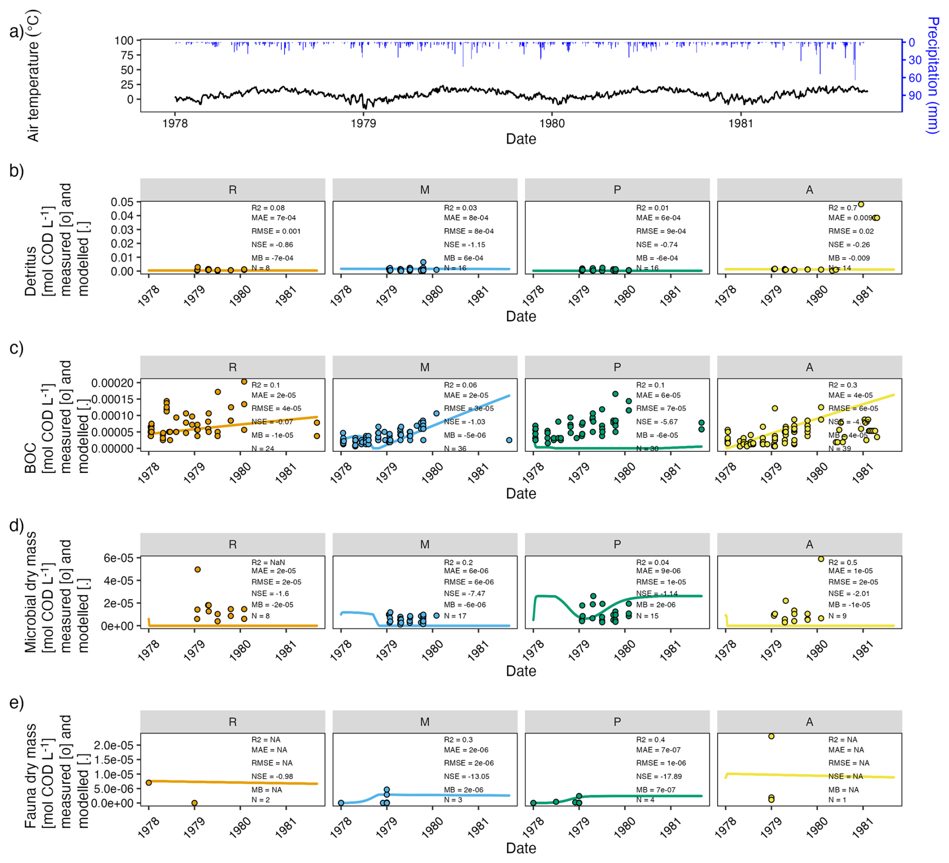
Figure 2 Visualization of the measured and modelled carbon compartments in the river Fulda floodplain for which Marxsen et al. (2021) had divided groundwater wells into four groups: river-near =  “R”, mixing zone = “M”, plume = “P”, agricultural area = “A”. (a) Air temperature (black) and precipitation in Fulda Horas meteorological station 1526 (blue) for the four years covering the study period. (b)–(e): measured (dots) and modelled (lines) carbon compounds in the four well groups (refer to text and Fig. 1). This scenario is referred to as the “Reference” scenario. Please note that the highest measured value in fauna dry mass (1.3 × 10⁻⁴ mol COD L⁻¹ in P03, group “R”; on 1 January 1979) was omitted from the plot to enable visualization of the modelled time course. In each subplot, 5 error measures and the number of values between measured data, averaged per group and date, and the model data are given.

The simulations (lines) in Fig. 2b–e reflect the measured values (points) well in general, even if the error measures indicated low quality, partly due to the low number of measured values. For BOC, the highest discrepancy between measured values and the modelled development, and the worst fit parameters, were found for the polluted zone “P”. We therefore used this model and changed only the parameters for the presence of fauna and for temperature in the scenarios of “no fauna” and/or “+1.5 °C”, and/or “+3 °C”, respectively (described below). The respective overviews of the same format as Fig. 2 are included in Sect. S8 in the Supplement: Figs. S3–S7.

The modelled detritus did not change much during the modelled time span (Fig. 2b). Event-based recharge in response to precipitation appeared to contribute little under the model assumptions (Fig. 2b). Modelled BOC first decreased then increased in the agriculturally-influenced “A” and the plume “P” zones (Fig. 2c). In the mixing “M” zone, after an initial increase, there was a decrease in BOC until autumn 1978 and then a steady increase. In the mixing “M” and the agriculturally-influenced “A” zones, BOC reached higher values at the end of the modelled time span than the measured values (Fig. 2c). The increasing trend was largely consistent with an apparent increasing trend in the in situ values over the study period (Fig. 2c).

The microbial dry mass initially decreased in the “R” and “A” zones and stayed at low levels (Fig. 2d). In the “M” and “P” zones, dry mass initially increased to the carrying capacity, which was set to be the maximum microbial dry mass measured per group. The dry mass more or less stayed on the carrying capacity or slightly below, for the better part of 1978, and then decreased. This decrease was only temporary in the “P” zone (Fig. 2d).

Modelled fauna dry mass (after an initial slight increase in zone “A”) slowly and steadily decreased in the river-near “R” and the agriculturally-influenced “A” zones (Fig. 2e). In the “M” and “P” zones, fauna dry mass increased until late autumn 1978, and then stayed on a level just below the carrying capacity (the highest measured fauna dry mass per group).

The scenarios for the simulations with increased temperatures and/or lack in fauna are given in Sect. S8 in the Supplement: Figs. S3–S7. The error metrics all indicate a worse-than-desired fit. In particular, for the fauna data for the groups river-near “R” and agriculturally-influenced “A” there were only data available from 1 or 2 dates, respectively, so that the error metrics could not even be calculated. The trend parameters of all scenarios are given in Sect. S10 in the Supplement: Table S2.

The modelled BOC, microbial dry mass and fauna dry mass showed only slightly different patterns in the “+1.5 °C” scenario (Fig. S4), but very different patterns in the “+3 °C” scenario (Fig. S6). The three “no fauna” scenarios (Figs. S3, S5, S7) showed seasonal patterns for faunal dry mass. At +1.5 °C, fauna decreased seasonally (Fig. S4). However, this did not seem to influence net microbial growth and net BOC degradation. At +3 °C, however, fauna seemed to break down to low levels in summer 1978 (Fig. S6), from which they hardly recovered in the following springs and stayed low afterwards. Due to the lacking faunal grazing, microbial dry mass reached highest values, even to the parameterized carrying capacity. In turn, the resulting BOC values after the 3.5 years were the lowest of all scenarios, particularly in the “R” and “P” zones.

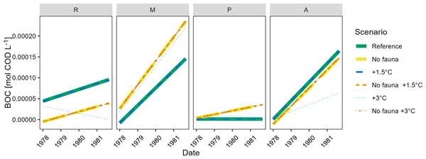
An overview over the start and end values of the modelled run, and of the linear fit, along with the fit parameters, is given in Sect. S10 in the Supplement, Table S2. The comparison of all trends is given in Fig. 3 for BOC, for microbial dry mass in Sect. S9 in the Supplement, Fig. S8, and for fauna dry mass in Sect. S9 in the Supplement, Fig. S9. In all zones, the three “no fauna” scenarios (“No fauna”, “No fauna +1.5 °C”, “No fauna +3 °C”) were indistinguishable from each other (yellow, bright orange and dark orange lines fall together). For the “M” and “P” zones, BOC trends rose to the highest values per zone, thus, highest BOC values remained in the system in the “no fauna” scenarios in these two groups (Fig. 3). Except for the “+3 °C” scenario in the “R” group and all “fauna” scenarios in the “P” group, BOC trends rose in all scenarios. In all four groups, the BOC trends for the “reference” and “+1.5 °C” scenarios were indistinguishable from each other. In the “P” zone, the “+3 °C” scenario also fell visibly into one line with the two other “fauna” scenarios. The main difference was thus not among scenarios of varying temperature, but among “fauna” and “no fauna” scenarios (Fig. 3).

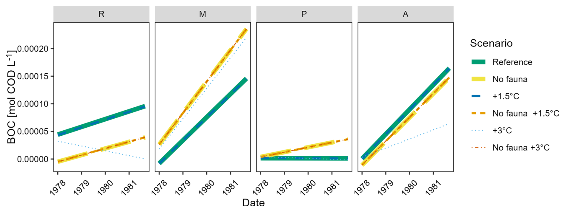
Figure 3 Trends through the modelled BOC in the river Fulda floodplain for the six scenarios which are given in the legend: “Reference”: input variables according to Marxsen et al. (2021); “No fauna”: setting all fauna variables to 0; “+1.5 °C”: raising all groundwater temperatures by 1.5 °C; “No fauna +1.5 °C”: setting all fauna variables to 0 and raising all groundwater temperatures by 1.5 °C; “+3 °C: raising all groundwater temperatures by 3 °C; “No fauna +3 °C”: setting all fauna variables to 0 and raising all groundwater temperatures by 3 °C. The four sub plots depict the four aquifer groups: river-near = “R”, mixing zone = “M”, plume = “P”, agricultural area = “A”; see text and Fig. 1.

The ecosystem service of carbon degradation was expressed as the concentration of mol COD of biologically oxidizable carbon BOC remaining in the system compared to the start value of the simulation, with column “Modelled concentration at end minus modelled concentration at time 0” being the difference between the columns “Modelled concentration at the end” and “Modelled concentration at time 0” (Sect. S10 in the Supplement, Table S2). We divided this difference by the value in column “Modelled concentration at time 0” to yield the value in the column “% change at end compared to modelled concentration at time 0”. BOC decreased by almost 100 % over the modelled period to very low values in the fauna scenarios in the plume “P” zone (Sect. S10 in the Supplement, Table S2), while it increased by over 700 % during the same period in the “no fauna” scenario in the mixing “M” zone. This shows that it depends on the start condition and measured microbial rates per zone what the outcome of the simulation will be – there is no general behaviour. We then related the “Modelled concentration at the end” of any scenario to the reference case to yield “factor by which modelled end concentration changed from reference modelled end concentration”. A value below 1 indicates a decrease in the respective concentration compared to the reference case. For BOC, this was observed in the “R” and “A” zones without fauna, and in the “R” and “P” zones at elevated temperatures, and at +3 °C additionally in the “A” zone (Sect. S10 in the Supplement, Table S2). In the “+1.5 and “+3 °C” scenarios, the remaining BOC increased only slightly above the reference level: with a factor of 1.37 in the “M” zone at +3 °C. In the “no fauna” scenarios, the remaining BOC increased by a factor of up to 6.6 in the plume “P” zone, compared to the reference scenario, regardless of the respective temperature increase (Sect. S10 in the Supplement, Table S2).

In partial agreement with the second hypothesis, an increase in temperature by 3 °C led to lower remaining BOC in most scenarios. However, an increase of 1.5 °C did now show a visible effect, except for the fauna dry mass. Microbial dry mass fitted trends increased beyond the reference case in the “no fauna” scenarios, except for the “P” zone. Fauna dry mass showed lower fitted slopes for the “+3 °C” scenarios in the “R” and “M” zones. The trends of faunal dry mass at “+3 °C” was different in every zone and (almost) fell together with the “no fauna” scenarios in the “P” zone. Clearly, a groundwater temperature increase by 3 °C had impacts on fauna which in the “R” and “A” zones led to increased microbial dry masses, which, in turn decreased remaining BOC trends in the “R” and “A” zones. The increase of temperature, however, cannot be assumed to act on all aquifers in the same way.

In order to deduce how sensitive the model was to changes in specific parameters, we conducted a regional sensitivity analysis separately for the four zones. k₁ was the most important or second most important only in three zones: “A”, “R”, and “M”, while microbial yield was the most or second most sensitive parameter in all four zones (Sect. S11 in the Supplement; Figs. S10–S13).

Since microbial yield on carbon and k₁ proved so sensitive, we ran the reference scenario (recent temperature, fauna present) with the minimum (0.0001; Fig. 4) and maximum (0.8; Fig. 4) microbial yield tested in the sensitivity analysis, and the minimum (0.000001; Fig. 5) and maximum k₁ (0.001; Fig. 5), to evaluate uncertainty. The fitted linear model trends for these extreme scenarios and the reference scenario for comparison are listed in Sect. S11 in the Supplement, Table S4.

High k₁ and low microbial yield led to the highest-per-group BOC values at the end of the model run (Figs. 4, 5, Sect. S11 in the Supplement, Table S4). With low microbial yield, BOC first decreased to low values (near-zero in zones “M” and “P”), but were higher than the reference at the end of the model run (Fig. 5). High yield, in contrast, decreased BOC in the “M” and “P” groups, and led to an initial peak in the “A” group, but at the end of the modelled period, the values were higher and close to those of the reference scenario (Fig. 5). Resulting BOC was visually higher in the low yield scenario than in the high yield scenario (Fig. 5). Where BOC increased, microbial dry mass declined to low values (Sect. S11 in the Supplement, Table S4). Fauna dry mass was higher in the high microbial yield “M”, “P”, and “A” zones than in the low microbial yield scenarios (Sect. S11 in the Supplement, Table S4).

Both the minimum k₁, i.e. minimum partitioning of detritus into biodegradable organic carbon, and the maximum yield, i.e. efficiency in transforming the taken-up BOC into microbial biomass, resulted in up to 100 times less BOC left over, depending on the group (Table S4). High k₁ and low microbial yield increased left-over BOC by a factor of up to 33, depending on the group (Table S4).

The uncertainty was high, particularly for the “M” mixing zone, when using extremely low and extremely high k₁ values (Fig. 4). Extremely low k₁ led to low concentrations of BOC to start with and consequently less BOC being left over after the simulation period, while extremely high k₁ led to a surplus of BOC.

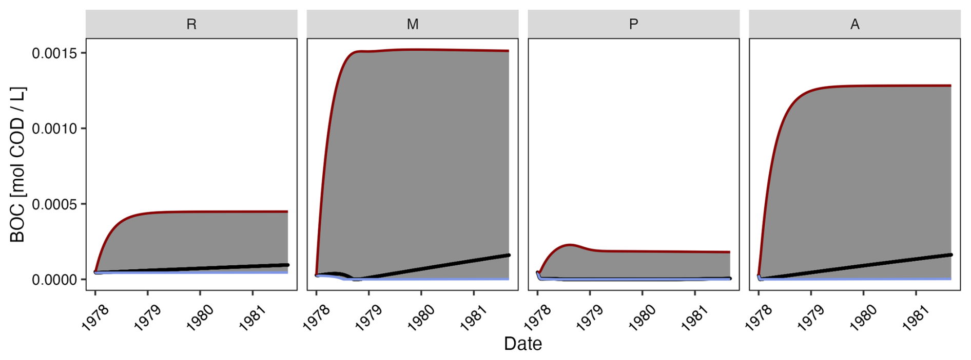
Figure 4 Model run of the reference scenario, as in Fig. 2 (black line), with the uncertainty range (grey polygon) between the scenario with the minimum value for k₁ tested in the sensitivity analysis (0.000001; light blue line limiting the grey uncertainty polygon) and the maximum value for k₁ (1; dark red line). River-near = “R”, mixing zone = “M”, plume = “P”, agricultural area = “A” (for the explanation of the zones, refer to text and Fig. 1).

In contrast, extremely low and extremely high microbial yield only resulted in a – narrow – uncertainty range around the scenario 1 for the groups “R” and “A” (Fig. 5). For the zone “P”, all three scenarios reached a minimum for BOC between mid 1978 and 1979 from which both extreme scenarios picked up earlier than the reference scenario. In the mixing “M” zone, the highest yield led to the slowest depletion of BOC, with a quick recovery of the BOC.

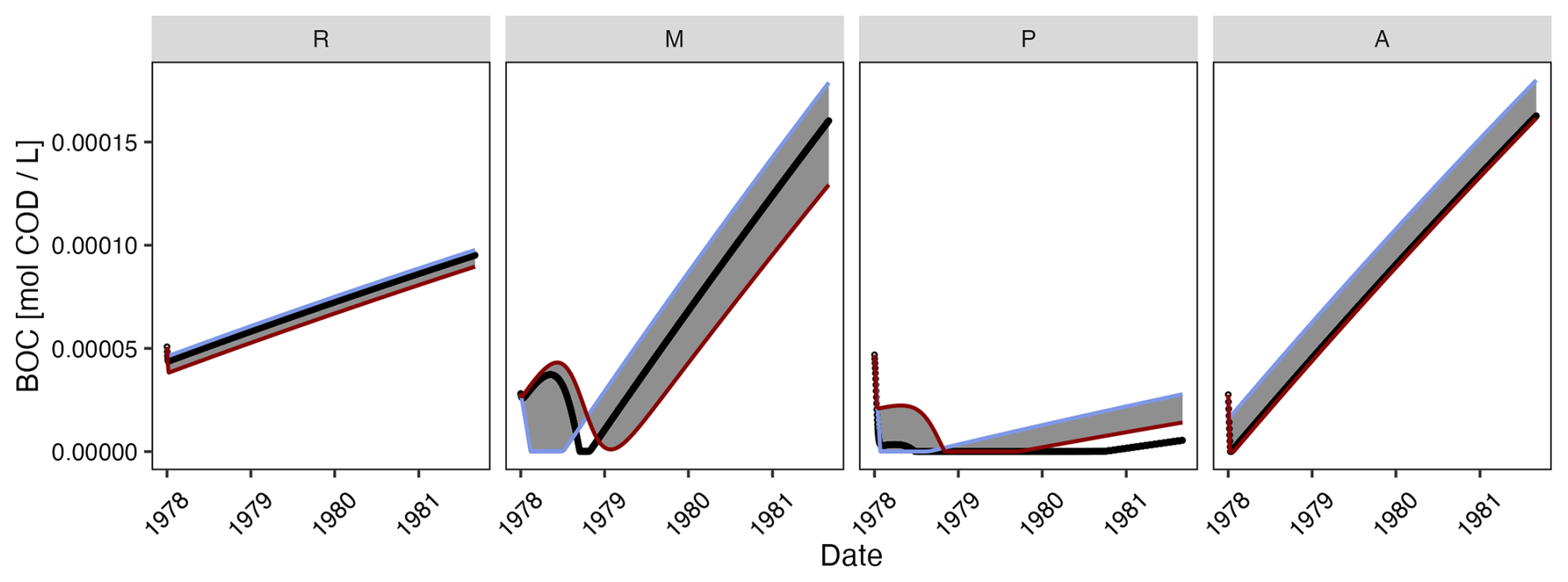
Figure 5 Model run of the reference scenario, as in Fig. 2 (black line), with the uncertainty range (grey polygon) between the scenario with the minimum value for microbial yield tested in the sensitivity analysis (0.001) and the maximum value for microbial yield (0.08). River-near = “R”, mixing zone = “M”, plume = “P”, agricultural area = “A” (refer to text and Fig. 1).

4 Discussion

This is to our knowledge the first attempt at developing a process-based proof-of-principle approach model of the groundwater food web, and it is the first endeavour at comparing scenarios of excluding fauna from the system. There have been laboratory studies exposing fauna to increasing temperature (e.g. Brielmann et al., 2011; Di Lorenzo and Reboleira, 2022; Spengler, 2017), but to our knowledge this has never been translated to a trophic dynamic model, even if restricting to the major part of the food web, as done here. One reason for such attempts not having been done before, lies in the difficulty of parameterizing such models. Our knowledge of the groundwater ecosystems' processes and dependencies is still patchy because field studies are usually conducted in hydrogeologically and hydrochemically heterogeneous aquifers with low numbers of monitoring wells, with sampling too rare in time so that local influences and site-specific parameters linked to variations in topography and geology superimpose effects from single variables such as temperature and oxygen (Koch et al., 2024a). Thus, the choice and development of appropriate parameters is crucial but virtually impossible based on the available field and laboratory data and to-date has to necessarily remain speculative. If the reference case is not appropriately parameterized, using it as a base for further scenarios is not reliable.

4.1 Modelling the reference case with fauna at the temperature of the observation period

Largely, the model set up, including the parameters, proved to be appropriate for representing the measured data. Modelled detritus in the reference case with fauna at the temperatures of the observation period stayed in the same order as most of the measured values and was a constant source of carbon in abundance.

Modelled BOC concentrations, designed to represent the bioavailable carbon fraction, mostly increased, and even beyond the measured values, over the investigated period of 3.5 years in the mixing “M” and the agricultural “A” zones. The model thus did not indicate a quasi steady state. This may be an artefact of the combination of model parameters and needs to be studied further. However, this increase was in the order of 0.00015 mol COD L⁻¹ over the investigated period of 3.5 years, while the highest values of detritus measured in the field were around 0.05 mol COD L⁻¹. Thus, this BOC increase was negligible for the catchment-scale budget. It just means that, seen over the whole 3.5 year modelling period, less of the biologically available carbon pool was taken up by microorganisms than was refilled from precipitation, physical breakdown, and import from the soil in the zones “M” and “A”. In contrast, in the polluted zone “P”, where measured values were as high as in zone “R”, the modelled BOC curve however approached 0 and did not rise visibly. One reason may be that the numbers of prokaryotes were high in the measured values, and were the highest in the model. Thus, similar amounts of carbon present in the area were taken up faster and to a higher degree in zone “P” by higher biomasses.

Assuming that the ecosystem in fact should have been in a quasi steady state, the trends would have been expected to be even closer to 0 in the reference model case, but for a simplistic food web model, we believe that the current approach is sufficiently close to the measured values. It further ensured that carbon was not limiting at the bottom of the food web over the whole period. This enabled comparison of the degradation of this resource being in over abundance. The less exchange with the surface, i.e. the deeper and the more secluded aquifers are, the more dependent on carbon import they will be (Schmidt et al., 2017; Schmidt and Hahn, 2012). Such scenarios will be part of the next questions to be addressed with the model.

In the scenarios, temporarily, modelled BOC was reduced to near-zero during the growth phase of the microorganisms (see below) in the mixing “M” and the plume “P” zones. This indicates feedback among the carbon fractions' concentrations – their scales seemed to be appropriate to reflect dynamic ecosystem behaviour. It also means that a longer-term simulation might have yielded different end concentrations and trends. This may be the subject of further model applications.

Modelled microbial dry mass showed (at least temporary) reductions to near-zero concentrations. In the “P” zone, dry mass rose to apparently the carrying capacity, dipped at the beginning of 1979 to low values and then rose again to apparently the carrying capacity. Fauna dry masses were lowest in the “P” zone (see below). In the “M” zone, the microbial dry mass rose very slightly to apparently the carrying capacity and then dropped at the end of 1978 to near-zero and never recovered. Also in the “A” and “R” zone, dry masses dropped to near-zero, already early in 1978, and never recovered. The fact that the dry masses in the “A” and “R” zones dropped so early, might reflect moments of feeding by higher-than-average fauna biomass (see below). The highest measured value for microbial dry mass had been observed in the agricultural “A” zone (compare Marxsen et al., 2021) and concurrently, carrying capacity was set to be at this high level, but was never nearly reached in the model with the current parameter set up. One reason for this may be that the modelled fauna dry mass stayed highest in the “A” zone compared to other zones and thus, fauna exerted grazing pressure, in this case reducing the microorganisms' capacity of degrading BOC, such as observed in Kota et al. (1999). This can be seen in the steadily rising modelled BOC. It is likely that the groundwater microbial community under agricultural land use exhibits growth and degradation characteristics much different from other zones (e.g. Dibbern et al., 2014), because subsurface carbon characteristics differ under the different land uses (Lehmann et al., 2021). It might be necessary to adapt the parameters and maybe even the model set-up for agricultural zones in future work. Another source of variation may be the distribution of organic carbon within the aquifer – in a porous environment, it might be physically separate from the microbial cells (Schmidt et al., 2017). To take such micro scale resource heterogeneity into account, requires a model which parameterizes at least two spatial dimensions (Schmidt et al., 2018), instead of the spatial 0D approach taken here.

Modelled fauna dry mass showed a steady increase within the first year in the mixing “M” and plume “P” zones, concurrent with a decrease in the microbial dry mass in the same zones, particularly towards end of winter in early 1979. With the end values being lower than the start values in the “R” and “A” zones, the fitted trends across the models were negative. The fauna fitted trends for the “+3 °C” scenarios decreasing to below 0 are an artefact. In the cases where the dry mass stayed at elevated levels over at least a certain period at the start, the drop down was steeper than in scenarios where fauna decreased at the beginning. The reason for the fauna dry masses not increasing later when the microbial dry mass was at carrying capacity, i.e. when food was presumably not limiting, e.g. in the “+3 °C” scenario, requires further investigation, but is most likely due to increased mortality of fauna at generally higher temperatures. Experiments on feeding and growth rates, building up on the published experiments on reproductive rates in Rütz et al. (2022) from central Germany, are still scarce and hardly available for middle-European temperate weather groundwater environments.

We had checked data from three studies for their potential use as parameters in the current model. These experiments had been conducted at 14 and 17 (Di Lorenzo et al., 2025b), at 15 (Navel et al., 2011), and at 10 °C (Mermillod-Blondin et al., 2025). Thus, only the study by Mermillod-Blondin et al. (2025) was under conditions somewhat comparable with the River Fulda floodplain. The study by Navel et al. (2011) was even conducted with a 12 h light 12 h dark cycle because of the studied interaction with a surface amphipod. Both elevated temperature (see above) and light (Simčič and Brancelj, 2007) may be stressful for stygobites though, and we did not deem the parameters appropriate for our model. This reduced the available parameters. Considering these caveats, for the sake of a first simplistic food web model, we considered the model set-up sufficient for the purpose.

4.2 Modelling the lack of fauna

In partial agreement with the first hypothesis, the “no fauna” scenarios in the “M” and “P” zones resulted in the highest remaining BOC, both in models, and in the fitted trend lines. In parallel, microbial dry mass was mostly highest in the “no fauna” scenarios. Less microbial degradation despite higher measurable dry masses points to a lack in rejuvenating grazing (Mattison et al., 2005). The bulk growth of microorganism was probably higher in the “fauna” scenarios, leading to higher degradation, but faunal grazing reduced the measurable microbial net dry mass (see also above). In addition to quantitative effects, grazing might also qualitatively change the microbial community (Longnecker et al., 2009) and might thus influence functions, and in the consequence, ecosystem services. As an example, groundwater crustacean abundance correlated with low-nucleic-acid (LNA) bacterial cells (Di Lorenzo et al., 2025a). This may hint to selective feeding (Jochem et al., 2004). HNA cells are often more metabolically active (Longnecker et al., 2005) and might thus be the preferred food source in grazing, leaving over microbial biomass less functionally active which then degrades even less carbon than the same dry mass of an un-grazed community might have done. Elucidating the actual microbial growth and uptake of organics per cell requires tracer studies (e.g. for marine systems: Zubkov and Tarran, 2008). It is interesting that this pattern emerges clearly from the rather simple food web modelling with the hybrid formula of combining the Monod model with the Verhulst model (Schlogelhofer et al., 2021).

The opposite effect of microbial uptake being reduced due to faunal grazing, described by Kota et al. (1999), was observed in the “R” and “A” zones. We lack understanding of the circumstances under which one pattern dominates. Also, the cited publications refer to grazing by protozoa, while we lacked quantitative field data for protozoa from the River Fulda floodplain and assumed that the grazing can be subsumed under a multicellular “fauna” dry mass term, based on the fauna appraisal in the River Fulda floodplain. To date, there is no field or laboratory study quantifying multicellular fauna, protozoa, and microorganisms in the same groundwater samples. Qualitative food webs were constructed based on molecular data in the Hainich aquifer (Herrmann et al., 2020).

Depending on the zone, remaining BOC concentrations decreased to the point of vanishing (plume “P” zone in the “+3 °C” scenario; discussed below), but increased in all other cases. This increase was up to more than 6.6-fold over the 3.5 year observation period. Without groundwater fauna, drinking water production will have to compensate by intensified treatment of organics which raises costs and insecurity.

4.3 Modelling an increase of groundwater temperature

It was surprising that an increase by 1.5 °C, while resulting in different fauna dry mass (except for the “P” zone), did not translate in different microbial or BOC fitted trends in the “fauna” scenarios. This may show that the lower grazing pressure from fauna was apparently compensated by faster microbial growth resulting in the net biodegradation of BOC being no different from the reference scenario. It might also have been a combination of the effect described by Kota et al. (1999) and thermally increased biodegradation rates. Fauna being clearly compromised by +3 °C translated into higher microbial dry mass. This higher microbial dry mass, however, did not alter BOC fitted trends in the “P” zone. Here, the diminished “rejuvenating” grazing might have compromised degradation, along with Mattison et al. (2005). The strongest increasing by 3 °C effect on faunal dry mass was seen in the “R” and “A” zones. In both zones, microbial dry mass fitted trends steeply increased over the course of the 3.5 modelled years, almost in parallel. However, the BOC fitted trends in these two zones were not parallel: it decreased in the “R” zone and increased in the “A” zone. In the “R” zone, thus, more remaining microbial dry mass degraded more, while in the “A” zone, it might have been a lack in rejuvenating grazing (Kota et al., 1999) again, which compromised degradation.

4.4 Modelling the lack of fauna at an increase of groundwater temperature

In contrast to the third hypothesis, the combination of increased temperatures and lack of fauna led to reduced degradation and higher remaining BOC compared to the reference scenario, only for the “M” zone at +3 °C. In that scenario, the difference to the BOC increase in the “no fauna at recent temperature” was negligible and thus, the reduced degradation was almost only due to lack of faunal grazing. In the “P” zone, the only factor shaping the BOC fitted trend was presence versus absence of fauna – temperature did not influence at all. The lack in temperature effects on fauna might partly be due to the overall low dry masses of fauna in the “P” zone.

While the faunal and microbial dry mass fitted trends were similar in the “R” and “A” zones, the BOC fitted trends diverged, particularly for the “+3 °C with fauna” scenarios. The reason may lie in different indirect effects which are hard to capture with the present set-up. More combinations of start conditions and parameters are needed to single out direct and indirect effects (Fišer et al., 2025).

BOC trends were lowest for the “+3 °C” scenarios in the “R” zone, and thus, the lowest BOC remained at the highest temperature with fauna, although fauna was clearly compromised. One explanation is that the “intermediate” disturbance caused by the temperature did, in this case, not lead to the highest diversity, as proposed in the original “intermediate disturbance hypothesis” (Connell, 1978), but to the highest ecosystem services. However, it needs to be tested how sustainable this pattern would be in the longer run under increased temperatures.

In general, the effect of losing fauna was mostly stronger than that of increased temperatures. The risk of losing fauna altogether increases with increasing temperatures, and thus, the risk of running into “no fauna” scenarios with partly clearly decreased degradation, increases.

4.5 Reduced ecosystem services

Here, we focused on degradation of BOC as a main ecosystem service relevant to drinking water production for humankind, as also demanded in Directive (EU) 2026/805. In some scenarios, particularly the “no fauna” scenarios of the “M” and “P” zones, the trends through the modelled BOC concentration increased more than the reference scenario over the study period. In other words, based on the fitted trends, the remaining carbon increased, which is an indicator of a reduced ecosystem service. Thus, the ecosystem service was reduced mainly under the lack of fauna. Losing groundwater fauna would mean losing a substantial part of the microbially-driven ecosystem service of carbon degradation.

This ecosystem service of degrading organic carbon comes at costs. E.g. the oxidation of carbon to CO₂ requires oxygen. There are a few laboratory studies quantifying the uptake of oxygen by groundwater fauna, e.g. Di Lorenzo et al. (2024), Hervant (1997), Hervant et al. (1998, 1999), Malard and Hervant (1999), and Mermillod-Blondin et al. (2008). Future studies should make dissolved oxygen a reaction partner in the organisms' uptake models, in order to evaluate where the provision of ecosystem services may be hampered by the aquifer's oxidation state. The wells in the Fulda aquifer which we used to parameterize the current models were largely fairly well oxygenated and dissolved oxygen was shown to be not limiting in Marxsen et al. (2021), but in other aquifer situations, dissolved oxygen played a major role in shaping communities (Strayer et al., 1997) and thus needs to be included in future models which should be applicable for other areas as well.

4.6 Sensitivity analysis

The two parameters showing higher sensitivity in one group each than other parameters were the microbial growth parameter yield and the k₁ (proportion with which detritus split into biologically oxidizable carbon). It is thus paramount to derive these two parameters carefully, to exclude artefacts, since we are showing here that changing microbial yield may change the outcome of the model considerably for BOC. After the study period, minimum k₁ and maximum yield had reduced the BOC left over from the feeding network, depending on the group, while high k₁ and low microbial yield had largely the inverse effect. There is thus high uncertainty for BOC, depending on these two most sensitive parameters. The uncertainty introduced from k₁ was high, particularly for the mixing “M” zone and extremely high k₁ values. The excess BOC was apparently not used by the food web and would be imported into drinking water production facilities, requiring more treatment than where the food web uses BOC efficiently.

The uncertainty from the tested range of the microbial yield was more complex and the four zones differed strikingly. The uncertainty was low for the groups “R” and “A”, meaning that different microbial taxa or different states of the taxa with a varying yield would not have led to high differences in remaining BOC. Changing the microbial community, e.g. by biostimulation or bioaugmentation would not have influenced the degradation much in these two zones. For the plume zone “P”, all three scenarios reached a minimum for BOC between early 1978 and mid 1979 from which both extreme scenarios picked up earlier than the reference scenario. All three scenarios would thus have led to a quite efficient use of BOC within the first year.

However, the low yield with high substrate use, and thus possibly steep biomass increase within the first months might have led to increased grazing by fauna which would, in turn, have kept a check on the increase of microbial biomass compared with the low yield and the reference scenario, leaving more BOC unused. In contrast, the high yield and thus low substrate use led to the latest minimum in BOC. The then low microbial biomass would have meant that fauna had less to graze than in the reference scenario, and the microbial biomass increased with a delay compared to the low yield scenario. The reference scenario kept the BOC at a minimum value for the longest time. Microbial biomass was using virtually all BOC introduced from detritus for the longest time, probably without losing too much biomass to grazing. This reference scenario would thus be the preferred scenario when trying to have good quality raw water for drinking water production.

In the mixing “M” zone as well, low yield with high substrate use, led to the fastest decrease in BOC, while high yield and thus low BOC use, led to the slowest decrease in BOC. After minimum values between 1978 and 1979, BOC concentrations again increased fastest with the low yield scenario, like in the plume “P” zone, probably for similar reasons. Here, however, the most effective scenario for keeping BOC low was the high yield scenario. The coinciding high substrate use under the “M” zone circumstances of the relationship between start concentrations of microbial biomass and BOC might have led to microbial biomass remaining low, but being just enough to sustain fauna which rejuvenated microbial growth optimally, depleting the resulting BOC concentrations. In follow up studies, the food web will be followed for a longer period, to check whether there are longer amplitudes in the growth and decline of BOC and microbial dry mass, than visible in the study period.

It needs to be noted though that particularly facultative oligotrophs are known to exhibit different growth parameters when facing different substrate concentrations (Ishida et al., 1982). This will be hard to parameterize representatively for an entire prokaryote community and questions how important exact microbial growth parameters can really be, and which uncertainty will remain even if parameterization has improved beyond this proof-of-principle study. It is hard to tell which process, physical degradation of complex organic molecules to become microbially palatable sources, or microbial efficiency (yield) is the most important. Because the growth parameters depend on substrate concentrations (Ishida et al., 1982; see above), an interaction between the two is more than likely. The form of the interaction will determine whether uncertainty will be a sum of the uncertainties of the two most sensitive parameters, or more or less than that.

4.7 Full budget

Full accounts of the productivity of groundwater systems with or without fauna, and at different temperatures, require incorporating CO₂ into the budget. While dissolved bicarbonate had been measured in the River Fulda aquifer study, some of the CO₂ (and CH₄ if produced; Herrmann and Taubert, 2022) will gas out. Such carbon loss from the system needs to be measured with the appropriate methods. Isotopes of the carbon atom may assist in such calculations (Schwab et al., 2019). A study on all carbon fractions in a groundwater ecosystem is still lacking – the AQUADIVA project (Küsel et al., 2016) offers probably the most complete data set on all compartments. But important grazer groups such as the rotifera (Ejsmont-Karabin and Karpowicz, 2025) and protozoa (Sinclair et al., 1993) require different sampling methods than the larger fauna and are thus often not included in quantitative groundwater grazer accounts. For a full budget of the standing stocks and processes in the groundwater ecosystem, these compartments need to be included in future field studies and in the models based on their results.

4.8 Necessary steps for further development

The error metrics between measured data and model fits were not satisfactory which was to be expected with the scant data base (low N of measured data). For the comparisons in the fauna data for the groups river-near “R” and agriculturally-influenced “A”, for which data were only available from 1 or 2 dates, respectively, the error metrics could not even be calculated. The overall low number of fauna data are the weakest point in this data set. This weakens of course the conclusions drawn from the modelling results for fauna. However, the field data show a wide variability which seems adequate when compared to field data from e.g. a 60 km² field site (Schmidt et al., 2007), a similar size field site in the River Isar valley (Brielmann et al., 2009) or from a region-scale investigation in Western Czechia (Schmidt et al., 2024b). Thus, we believe that the range of fauna abundances would have been not much larger with more frequent sampling data available. The trends over time cannot be evaluated with the in situ data set, but the modelled trends reflect what has been measured in monthly data e.g. in Schmidt et al. (2007). We thus assume that the sampled data and the modelled time course are representative for what was really happening, until more comprehensive data show the opposite.

We hope that this lack in fit prompts the necessary investigations and improvements on the model in more comprehensive studies following on this proof-of-principle study. In particular, it is important to reflect the traits (Hose et al., 2022) of not only the common and rather well-studied stygoxenes and stygophiles, but also of stygobites, and the proportion with which they occur, in the model parameters, to show robustness of the approach. The data necessary for such assessment are lacking.

In this modelling study we considered different kinds of energies as equal, due to a lack in better knowledge and data. This approach may lead to errors (Odum and Odum, 2000). Odum and Odum (2000) suggested to express everything in an ecosystem in the solar energy used to make each item. However, in an ecosystem where the sun does not shine, and where instead not only the import of plant material, but also chemolithoautotrophy without solar energy provide resources at the basis of the food web (Herrmann et al., 2015; Kellermann et al., 2012), compromises must be found.

Many temperature-related processes are not considered here, namely environmental changes, such as lower solubility of dissolved oxygen, higher dissolution of ions (Retter et al., 2020), all of which may be detrimental to organisms. Thus, the net optimum for groundwater microbial activity is probably lower than the physiological activity optimum itself. However, we lack parameters for groundwater ecosystems to include such dependencies into models.

This study was based on a plethora of assumptions most of which might trigger discussions. Also, here, only average compartment carbon concentrations were modelled. It is relevant to focus on the whole range of likely conditions, i.e. including minima and maxima. However, because of error propagation, this is not a straightforward process and requires diligent development. The present study aims to serve as a starting point for future developments.

Climate change does not happen everywhere in the same way – it not only translates into increased temperatures, but also into changed recharge patterns which were not considered here. One next step is to use spatially resolved temperature scenarios and chemical reaction solvers such as PHREEQ-CE to extrapolate groundwater ecosystem services under climate scenarios to the national, continental, and global scale.

5 Conclusions

This first proof-of-principle study on quantifying the change in ecosystem services at scenarios of lost groundwater fauna, and of increased temperature, showed that the partial loss of ecosystem services (here: organic carbon degradation) due to lacking fauna increased remaining organic carbon up to 6.6-fold, based on the 3.5-year observation period. While there were differences among aquifer zones that were characterized by differing patterns in nutrient and carbon background, some general patterns emerged for all four groups of studied wells. This increased confidence in the model, so that we began changing parameters and/or excluding fauna biomass to run scenarios representing warmer climates, and comparing the ecosystem function degradation of organic carbon when fauna is present versus absent. These in silico manipulations showed that the lack of fauna could potentially strongly affect water quality and thus costs for drinking water production. This means that biomanipulation by protecting and promoting groundwater fauna for improving water quality, might be a promising concept.

The fauna's role in groundwater purification might in general still be underestimated. This has implications for drinking water production which will locally have to compensate the lack of fauna's ecosystem services by increased treatment which raises costs and insecurity. We hypothesize that sustainable drinking water production that is foremost based on reducing organic carbon is more reliable and less costly when groundwater fauna in the production area more active.

To address such hypotheses, particular efforts will have to be spent on the variables and parameters. Those used in this modelling exercise will have to be confirmed and adapted by more detailed field studies to ascertain transferability of the model to other regions, other biogeochemical conditions, and other resident fauna. Particularly, the data from the river-near Johannisaue area might not be representative for aquifers in other topographies, hydraulic exchange situations, and geological strata. More adequate data with which to parameterize process-based models are urgently needed.