Biome classification across global vegetation models reveals consistent biome shifts under future climate change

Climate change is altering ecosystems and will reshape the global distribution of biomes. These shifts can significantly influence biodiversity, ecosystem functions and services that are essential for human livelihoods. Robust assessments of future biome dynamics are therefore urgently needed. Here, we aimed to robustly quantify and map future biome shifts under climate change using a reproducible, multi-model ensemble approach. We employed random forest models to classify outputs from five global vegetation models (GVMs) into 31 observation-based biome maps representing land cover under current climate conditions. Model-derived biome maps showed strong agreement with observation-based maps (average κ=0.77 for 31 maps), with higher agreement for biomes with well-known temperature constraints. Then we used the random forest models and GVM simulations for future climate conditions to infer future biome distributions, and we evaluated potential biome shifts for each GVM-biome map combination under three climate change scenarios (RCP2.6, RCP6.0, RCP8.5, 403 maps in total). Across all scenarios, GVMs projected biome shifts until the end of the century, where the likelihood of change increased with the level of climate change in RCP scenarios. Between 4 % and 56 % of the land surface were projected to undergo biome transitions in the full model ensemble of 403 different combinations of GVMs, RCPs and observation-based biome maps used to create biome maps. Broad spatial patterns of biome change were consistent across models. Biomes in cold regions were most susceptible to biome shifts, as boreal and temperate biomes shifted poleward, following temperature change. Equatorial rainforests remained largely stable, while other studies found forest dieback. These findings highlight regions and biomes most susceptible to future climate change, even under the low-emission scenario RCP2.6. Overall, we developed a multi-model GVM ensemble of future biome projections, based on a unified and reproducible biome classification approach. This approach allows quantification of uncertainties related to biome classification schemes across multiple GVMs and RCP scenarios, and it can be applied to any vegetation model. We provide critical insights for targeted climate mitigation and adaptation strategies and conservation of the remaining natural vegetation.

1 Introduction

Climate change is already affecting ecosystem dynamics, their biogeographic distribution, and thereby the provision of ecosystem services that are essential for human societies (Parmesan et al., 2022). In turn, changes of the land surface can influence climate via biophysical feedbacks (Bonan, 2008). Future climate change is expected to strengthen such impacts, and result, for instance, in drought-induced tree mortality (McDowell et al., 2018), enhanced fire danger (Hetzer et al., 2024), or threats to ecological networks (Schleuning et al., 2016). A robust assessment of potential changes of ecosystem dynamics and ecosystem services is therefore urgently needed to inform conservation and climate change mitigation and adaptation. Biomes, large-scale vegetation formations defined by their functional or structural features (Mucina, 2019), have often been used as units to assess vegetation change (e.g., Bonannella et al., 2023; Tobian et al., 2024; Huntley et al., 2023). Biomes are typically well associated with the prevailing climatic conditions due to bioclimatic limits such as chilling requirements or frost tolerance (Prentice et al., 1992), as well as with natural disturbance regimes that constrain the spatial distribution of biome-specific species. Biomes have been associated with important ecosystem services such as carbon storage, climate regulation, or biodiversity (Parmesan et al., 2022). Here, we aimed to robustly quantify and map future biome shifts under climate change using a reproducible, multi-model ensemble approach.

Assessing future biome change is complex, as different drivers of their distributions interact and may have contrasting effects on their distribution. For instance, in tropical savannas, increases in atmospheric CO₂ and CO₂ fertilization of C₃ photosynthesis may enhance woody encroachment and transitions towards woodland and forest (Midgley and Bond, 2015), while increasing drought or changes in fire regimes due to management or changes in fire conditions may counteract woody encroachment (Scheiter and Savadogo, 2016). In boreal forests, warming may enhance growing season length and photosynthetic rates, which are all strongly controlled by temperature, and hence forest expansion (Lucht et al., 2002). Climate model-derived future projections of temperature changes show more consistent global patterns than those for precipitation changes, which are more uncertain (Shi et al., 2021). Both temperature and precipitation changes are expected to cause vegetation changes and shifts in biome patterns. Yet, under the current climate model projections with more consistency in temperature change than in precipitation change, we expect that boreal forests and other biomes with clear temperature-related bioclimatic limits should respond more consistently to climate change across different climate change scenarios than biomes primarily limited by moisture or disturbances, or those without clear bioclimatic limits. In addition to climate, land use and management have substantially transformed biome patterns, and a large proportion of the land surface is covered by non-natural biomes (Fischer et al., 2022). Direct anthropogenic impacts, such as transformation into cropland, can override any climate change-induced biome change.

Global vegetation models (GVMs, Prentice et al., 2007) have been used to study the potential impacts of climate change on biome distributions, ranging from the regional (e.g., Scheiter et al., 2018) to the global scale (e.g., Gonzalez et al., 2010). Such comparisons are, however, associated with different sources of uncertainties. GVMs differ in the representation of ecological processes, plant functional types (PFTs) and disturbances such as fire or drought-induced mortality, and how PFTs are parameterized, such that simulations of current vegetation patterns and responses to climate change differ between models (Smith et al., 2014; Sitch et al., 2008). Further, the biome type of a grid cell is typically not a model output variable but derived in a post-processing step. Using model state variables such as leaf area index (LAI) or cover fractions of different PFTs and biome-specific thresholds for those state variables, modeled vegetation is classified into different biomes. For instance, in a classification scheme typically used for LPJ-GUESS, a tree LAI above 2.5 and dominance of the tropical evergreen tree PFT represent tropical rainforest (Hickler et al., 2012), and in aDGVM, tree cover of more than 80 % is typically categorized as forest (Martens et al., 2021). Model variables, thresholds and biome types used in different studies and GVMs are commonly not unique and to some extent arbitrary, and may differ between studies. This makes direct comparisons of modeled biome patterns and biome change difficult. We argue that a reproducible biome classification applicable to any GVM is required to facilitate multi-model comparisons of future biome shifts and a quantification of uncertainties related to biome classification. Dallmeyer et al. (2019) therefore harmonized functional types and biomes to enable comparisons of modeled biome distributions, and Champreux et al. (2024) proposed a method to aggregate biome types to allow comparisons of biome schemes with different numbers of biome types.

A further caveat for analyzing modeled biome distributions and to evaluate models based on observation-based biome maps is that multiple observation-based biome or land cover maps were developed (see Beierkuhnlein and Fischer, 2021; Fischer et al., 2022,  for overview). These maps differ in the quantities used for classification, in the number and definition of biome types included in the maps, and their spatial patterns. For instance, the Olson et al. (2001) and Dinerstein et al. (2017) maps are based on biogeographic zonation and species distributions, and the Whittaker and Likens (1975) is based on temperature, precipitation and plant community distributions. More recent biome maps were often informed by remote sensing products. For instance, Buchhorn et al. (2020) used multi-spectral reflectance data, and Higgins et al. (2016) used a range of products including productivity and height. Biome maps are widely used in climate change and biodiversity research. For instance, the Olson et al. (2001) map is often used for biome-specific analyses (e.g., Newbold et al., 2016) or as a reference map in international initiatives such as Intergovernmental Science-Policy Platform on Biodiversity and Ecosystem Services (IPBES) or World Wide Fund For Nature (WWF). Champreux et al. (2024) showed that disagreement between biome maps is generally highest in areas with moderate vegetation cover and strong anthropogenic impacts. The biome classification scheme applied to GVM results and the observation-based biome map used for data-model comparisons can therefore influence data-model agreement and projected rates of biome shifts under future climate conditions (Scheiter et al., 2024a). Misclassification of biomes may result in inappropriate conclusions for conservation and management policies for ecosystems (Kumar et al., 2020).

These uncertainties and caveats make it difficult to provide an objective comparison of potential biome change across different GVMs. To achieve robust and comparable projections of biome shifts and quantify uncertainties in biome projections across GVMs, climate change scenarios and existing observation-based biome classification schemes, we first developed a novel and reproducible biome classification framework. Specifically, we used machine learning (random forests) for a reproducible biome classification based on the LAI distribution simulated by five GVMs and 31 observation-based biome maps provided by Fischer et al. (2022). All GVMs were run following the protocol of the Inter-Sectoral Impact Model Intercomparison Project phase 2b (ISIMIP2b) using the same environmental forcings (Frieler et al., 2017) and fire enabled, but correcting for anthropogenic land use to represent only natural vegetation biomes. We applied supervised classification to classify annual LAI of different PFTs simulated by the GVMs under current conditions (2006 to 2020) into each of the 31 biome maps. Even though a variety of variables such as vegetation cover, vegetation height or productivity is available for the GVMs and suitable for biome classification, we only selected LAI. This variable is directly simulated by GVMs, observable globally, and it is a core biophysical variable in GVMs, linked to canopy structure, light availability and productivity. It has also been used for biome classification in GVMs (e.g., Smith et al., 2014) and our analyses are therefore consistent with previous studies. Using our novel classification approach, we assessed the agreement between all combinations of GVM- and observation-based biome maps, and agreement of potential biome change until the end of the century (2085–2099) under three climate change scenarios (RCP2.6, 6.0 and 8.5) to identify the areas with biome stability and areas most susceptible to biome change. We used regression models to relate the susceptibility to environmental drivers. As temperature changes are more consistent in climate change projections (Shi et al., 2021), and PFTs in GVMs are often defined by temperature-related bioclimatic limits, we expected more consistent responses to temperature than to precipitation, and in biomes associated with temperature-related bioclimatic limits. The representation of plant hydraulics and drought-induced tree mortality are a source of uncertainty in many GVMs, limiting the model's capacity to simulate responses to precipitation change, particularly drought, and temperature effects on vapor pressure deficit (VPD). In addition to GVM results, we applied random forest models to classify observation-based PFT maps into biomes (Tuanmu and Jetz, 2014; Harper et al., 2023), and we compared the performance of classifications based on GVMs and observation-based PFT maps. While GVM uncertainties related to different climate forcings (Ahlström et al., 2012), climate change scenarios (Martens et al., 2021; Tobian et al., 2024), and the representation and parametrization of vegetation (Pappas et al., 2013) have been analyzed in previous studies, we address uncertainties related to the post-processing step of biome classification, by eliminating model-specific biome classification rules and applying a consistent, observation-informed scheme across models.

We hypothesize that (1) observation-based biome maps can be reproduced using GVM results, but we expect that agreement between modeled and observation-based biome maps (quantified by κ statistics) differs between GVMs and biome maps used to inform biome classification; (2) accordingly, the extent of biome change until the end of the century differs between GVMs, while the broad spatial patterns of biome stability and susceptibility to biome change are consistent between GVMs, (3) model performance (i.e., κ statistics) is better for biomes where the boundaries are largely driven by relatively well-understood temperature limits, because temperature-related bioclimatic limits in the models constrain the extent of PFTs and accordingly of biomes, and (4) future projections are more consistent for biomes with well-understood temperature limits, because of the robust trends of temperature change in the climate change scenarios used in our analysis.

2 Methods

2.1 Data

GVM simulation results were obtained from the ISIMIP repository (https://data.isimip.org, last access: 14 November 2025, see Table S1 for summary of all data sets used for the analysis). Specifically, we used simulation results from ISIMIP2b simulations for the climate change scenarios RCP2.6, RCP6.0, and RCP8.5, simulated with climate forcings from IPSL-CM5A-LR or HADGEM2-ES Earth System Models (ESMs, Frieler et al., 2017; Reyer et al., 2024). Both climate forcing data sets were bias corrected with EWEMBI observational data (Lange, 2018, 2019). ISIMIP2b simulation runs include different combinations for direct anthropogenic impacts and atmospheric CO₂ (increasing or fixed). Here, we used the scenario where land use, nitrogen deposition and fertilizer input was included but fixed at the levels of the year 2005 (“2005soc” scenario in ISIMIP repository) and where CO₂ increased according to the respective RCP scenario (“co2” scenario in ISIMIP repository). We selected the combination of IPSL-CM5A-LR, “2005soc” and “co2”, because for this combination, results were available for five different GVMs for RCP6.0. This combination of scenarios had the highest number of GVMs available, ensuring model comparability. Model results were available for LPJ-GUESS (Smith et al., 2014), ORCHIDEE (Guimberteau et al., 2018), ORCHIDEE-DGVM (Guimberteau et al., 2018), CLM4.5 (Thiery et al., 2017), and CARAIB (Minet et al., 2015; Warnant et al., 1994; Dury et al., 2018). For RCP2.6 and RCP8.5, we used HADGEM2-ES results for CLM4.5, as results for IPSL-CM5A-LR were not available in the repository. For RCP8.5, results were only available for LPJ-GUESS, ORCHIDEE and CLM4.5. As we did not run model simulations for this study but only used available model results, we do not provide model descriptions or model comparisons and refer to the key references for the different models (Supplement Sect. S1, Tables S2 and S3 for temperature-sensitive parameters and bioclimatic limits in the GVMs).

The target variable for biome classification was leaf area index (LAI), because this variable has historically been used for biome classification (e.g., Hickler et al., 2006; Smith et al., 2014). Using LAI ensures consistency with previous studies. The GVMs simulate state variables such as carbon pools, height or LAI separately for each PFT in response to environmental conditions, competition and disturbances such as fire (Prentice et al., 2007). The cover of different PFTs within grid cells can be static and informed by land cover maps (ORCHIDEE, CLM4.5) or change dynamically in response to biotic and abiotic factors (LPJ-GUESS, ORCHIDEE-DGVM, CARAIB). For our analyses, we only used PFTs representing natural vegetation while bare ground and anthropogenic PFTs were ignored (see Supplement Sect. S1 for details). Annual LAI data were averaged for the 15-year periods 2006–2020 and 2085–2099, representing early and late conditions within the future simulations of ISIMIP2b that were provided for the period 2006–2099 for each climate scenario. Climate conditions in different RCPs do not differ strongly for the early period (2006–2020) but diverge after that period. Therefore, we hereafter denote the early period as “current” irrespective of the RCP scenario, and the late period as “future”. LAI data in the ISIMIP repository did not account for cover fractions of different PFTs within grid cells. Therefore, we processed LAI data in two steps. First, we multiplied PFT-specific LAI with the cover fraction of the respective PFT. Then, we scaled the LAI of natural PFTs with the inverse sum of the cover fractions of all natural PFTs. The second scaling step removes anthropogenic PFTs and assumes that the entire grid cell is only covered by natural PFTs (see Supplement Sect. S1 natural/anthropogenic PFTs). This scaling is reasonable, as we only consider natural biome types in our biome classification (see section “Biome classification”), while all anthropogenic PFTs and land cover types are excluded. The data were available at 0.5° spatial resolution.

We used 31 biome maps compiled by Fischer et al. (2022), hereafter called F31 biome maps. Those maps were published between 1964 (Walter, 1964, with adjustments and revisions afterwards) and 2020 (Allen et al., 2020), and represent historic biome patterns observed before the publication date. Biome states may have shifted since the publication date. Yet, as the time period represented by the biome maps is not always clearly defined and as we use 15-year periods for GVM results, we ignored potential biome shifts after the publication of biome maps and compared all maps to the GVM results for current conditions (2006–2020). The approach is consistent across all observation-based biome maps, even though it may introduce minor uncertainties due to mismatches in the time periods. The biome maps were derived from different quantities and by different methods, such as biogeographic mapping of species, bioclimatic zonation or classification using remote sensing data. Hence, the biome maps represent different functional and structural features of vegetation. The maps differ substantially with respect to the number of biomes included, the definition of different biome types, and accordingly their spatial distributions. As GVM results from the ISIMIP2b repository were provided at 0.5° spatial resolution (see previous paragraph), we aggregated the biome maps to the same 0.5° resolution using the nearest neighbor method. In our analysis, we created random forest models for each combination of the 31 observation based biome maps and the GVMs and did not aggregate them into consensus biome or GVM maps. This approach is necessary because the biome maps and GVMs use incompatible biome and PFT types, respectively. Aggregation into consensus maps would itself require a series of subjective decisions and would introduce additional uncertainty. Further, our approach allows us to explicitly quantify uncertainties related to biome classification.

In addition to GVM results, we used observation-based PFT maps for our analysis: the European Space Agency (ESA) Climate Change initiative (CCI) product (Harper et al., 2023) and the Tuanmu and Jetz (2014) product. The products include different sets of PFTs (Supplement Sect. S1). Those PFT maps were derived from different remote sensing products. Harper et al. (2023) developed a cross-walking scheme to match PFT distributions with land cover classes from the CCI Multi-Resolution Land Characteristics (MRLC) product, supported by products describing for example surface water, built-up areas or tree canopy cover and height. Tuanmu and Jetz (2014) used classification and data integration approaches to create a consensus map based on reflectance data from GlobCover Land Cover (GlobCover), Moderate Resolution Imaging Spectroradiometer (MODIS2005), Global Land Cover 2000 (GLC2000) and IGBP Data (DISCover). Even though those products are observation-based, they are expert-based and subjective and affected by uncertainties (Wang et al., 2023). Classification with those products serves as reference for the evaluation of GVM results. Those maps are only available for current conditions, while future changes of PFT maps are not available. Both products were aggregated to the 0.5° spatial resolution of the GVM results using bilinear interpolation.

2.2 Biome classification

We used random forests to classify PFT information from GVMs (based on LAI) or remote sensing (cover fraction) into the F31 observation-based biomes, that is, we applied supervised classification. Random forests were fitted using the “randomForest” R package (version 4.7-1.2, Liaw and Wiener, 2002). For each combination of one of the F31 biome maps, modeled LAI or observation-based PFT cover map, and RCP scenario, one random forest model was created. Simulated LAI for current conditions or cover fractions were used as explanatory variables, the biome types of the respective biome maps were used as response variables, where all biome types were classified in one random forest model. We used the “randomForest” default settings. For each random forest, 2500 trees were created. Model performance was evaluated using out-of-bag (OOB) error estimation for each tree, therefore we did not split data into training and testing subsets. Using the random forests, we then predicted biome patterns for current conditions for each GVM or PFT map and for each of the F31 biome maps. Overall, we created 62 biome maps for PFT products (31 biome maps, 2 PFT products), 155 maps for five GVMs for RCP2.6 and RCP6.0, and 93 maps for three GVMs for RCP8.5. We further applied the random forest models to the PFT-specific LAI simulated by GVMs for future (period 2085–2099) climate and CO₂ conditions of the respective GVM, to obtain biome patterns for future conditions. This was only possible for the five GVMs, as future projections for the PFT cover products were not available. Overall, we created 403 biome maps for different combinations of GVMs, RCPs and F31 biome maps for both current and future conditions.

2.3 Analyses

For comparisons between observation-based biome maps (Fischer et al., 2022) and the biome patterns obtained from random forest models trained on the respective biome maps, we used the κ-statistics (Monserud and Leemans, 1992). This quantity allows comparisons between the spatial patterns of categorical variables and considers that agreement can be caused by random effects. Values in the range 0–0.2 indicate slight agreement, 0.2–0.4 fair, 0.4–0.6 moderate, 0.6–0.8 substantial and 0.8–1 almost perfect agreement. We created maps to identify areas where the F31 and respective modeled biome maps agree or disagree, and assessed the relationship between κ values and the number of biomes in the respective biome map. We further calculated κ for each biome type in each F31 biome map and related it to the number of grid cells covered by the respective biome type, to analyze if the performance of the random forest model was related to biome coverage. Therefore, the target biome type was set to one while all other biome types were set to zero, and κ values were then calculated based on the binary maps. We assumed that the entire 0.5° grid cell is covered by only one biome type, both in the F31 maps and the model results. For these analyses of model performance under current climate conditions, we present only results from the RCP6.0 scenario, as vegetation simulations for the current period and agreement with observation-based biome maps are similar.

For the GVM results, we analyzed the susceptibility to biome change under future climate and CO₂ conditions for the entire ensemble of GVM and biome maps and regions of biome stability. Therefore, we created maps indicating biome change or stability between current and future climate conditions for each GVM and for each of the F31 biome maps. Hence, we obtained 155 maps of biome change (5 GVM × 31 biome maps) for RCP2.6 and RCP6.0 and 93 maps for RCP8.5. These maps were then overlaid and the number of models projecting a biome change was counted. Values approaching 155 or 93 indicate that all models consistently predict biome change whereas low values indicate that models consistently predict biome stability. We denote the number of models projecting biome change as the susceptibility of biome change. A high number of GVM-biome-map projecting a biome change in a grid cell is associated with a high susceptibility of biome change, accordingly, a low number is associated with low susceptibility and biome stability. For visualization, we categorized these results, where “low” indicates that 0 % to 20 % of the models predict a biome change (representing low susceptibility and stability), “Medium” indicates 20 % to 40 %, “high” indicates 40 % to 60 % and “very high” more than 60 %. We assessed if the proportion of grid cells affected by biome change was related to the agreement between data and model results (i.e., to the κ value) or to the number of biomes in the respective biome map.

We used a linear regression to test if the number of grid cells affected by biome changes can be explained by the RCP scenario, GVM, F31 biome map, and number of biomes in the biome map. In this analysis, spatial information was aggregated into an average value for each combination of F31 map, GVM and RCP. To identify main drivers of biome change at the grid cell level, we modeled the susceptibility to biome change using a Random Forest (RF) regression using the “ranger” R package (version 0.16.0, Wright and Ziegler, 2017). Data from RCP2.6, 6.0, and 8.5 scenarios were modeled both individually and in a joint model to capture response patterns across all scenarios. Predictors were current (2006–2020) temperature and precipitation, anomalies between current and future (2085–2099) climate (Figs. S1, S2), and geographic coordinates. To isolate the susceptibility to biome change in different temperature zones, we also used the current temperature zone as predictor (cold <5 °C, temperate 5–18 °C, warm >18 °C). Relative driver influence was assessed via permutation importance, and an interaction model was used to statistically validate sensitivity differences across temperature zones. To isolate responses to temperature change, we created partial dependence plots between biome change susceptibility and temperature change for the three temperature zones.

2.4 Olson et al. (2001) map as an example

To exemplify modeled biome distributions and biome change, we analyzed the results for the Olson et al. (2001) biome map in more detail. We selected this map as it is commonly used as reference biome map, for example in IPBES or in biome-specific analyses (e.g., Sanderson et al., 2002; Loarie et al., 2009; Newbold et al., 2016). We created maps showing the current and future biome patterns, agreement between modeled and observation-based biome distributions, as well as maps indicating regions where biome shifts occur. To quantify the agreement per biome, we calculated contingency tables for each model indicating the percentages of overlap between observation-based and modeled biomes. In addition, κ values were calculated per biome by setting grid cells covered by the target biome to one and all other biomes to zero, and then calculating the κ value for the binary map. We created Sankey plots to illustrate transitions under biomes between current and future conditions using the “ggsankey” package (version 0.0.9999, Sjoberg, 2024), and quantified biome coverage and transition rates for current and future biome distributions.

To test if agreement between modeled biomes for current conditions and the Olson et al. (2001) biomes is higher for temperature-driven biomes, we first split the biome types into those mainly driven by temperature and those driven by other factors (Table S4). This classification is based on literature and expert-knowledge of the authors, and other authors may use another classification. We did, however, not test the sensitivity of our results to this classification as we used random forest regressions to analyze biome changes for the full model ensemble in response to multiple predictors (see previous section). Then, we calculated the mean κ values for both groups and all GVM and PFT maps. To test if the likelihood of biome change differs between biomes mainly constrained by temperature or other factors, we calculated the percent of grid cells predicted to undergo biome change for both groups. In contrast to the temperature-related analyses of the full ensemble including all 31 biome maps (Sect. 2.3), this approach tests temperature responses indirectly via assumptions on temperature sensitivity of biomes.

To test if biome change is more consistent for biomes with well-defined temperature limits such as chilling requirements or frost tolerance used to define PFTs, we used the coefficient of variation as proxy for consistency. Specifically, we calculated for each GVM and each biome transition the respective percent of grid cells affected by this biome change. Then we calculated mean, standard deviation, and coefficient of variation of these percentages for each biome change across the GVMs. To account only for relevant biome change, we excluded those with less than 5 % coverage under current conditions. Finally, we used a t-test to compare mean coefficient of variation for biomes with well-defined temperature limits and biomes explained by other factors. If biome change for temperature-defined biomes are more consistent, we would expect lower coefficients of variation.

All analyses were conducted using R (version 4.4.2, R Core Team, 2024). Spatial data were processed using the “terra” (version 1.8-10, Hijmans, 2024) package. Figures were created using the “ggplot2” (version 3.5.1, Wickham, 2016) package. All R scripts are provided in Scheiter (2026).

3 Results

3.1 Biome classification

Data-model agreement varied strongly across the 31 biome maps (Fischer et al., 2022) and different LAI or PFT data used for the biome classification (Fig. 1). Overall, κ values were higher for biome classification using observation-based PFT data (mean κ=0.95, indicating almost perfect agreement) than for LAI data simulated by GVMs (mean κ=0.77, indicating substantial agreement). Of the F31 biome maps used to inform the biome classification, agreement was highest for the Schultz (2016) biome map when averaging κ for all GVMs (κ=0.83), for the The Nature Conservancy (2009) map for GVMs and PFT maps combined (κ=0.87), and for the Buchhorn et al. (2020) biome map using only the observation-based PFT maps for classification (κ=0.98). The lowest overall performance was obtained for the Tateishi et al. (2011, 2014) map (κ=0.75). The relation between the κ values and the number of biomes included in the F31 biome maps was weak (Fig. S3, Table S5). The κ values per biome were related to the fraction of grid cells covered by the respective biome, i.e., biomes with large cover had a higher κ values, while biomes with smaller cover showed large variation of κ values ranging between zero and one (Fig. S4).

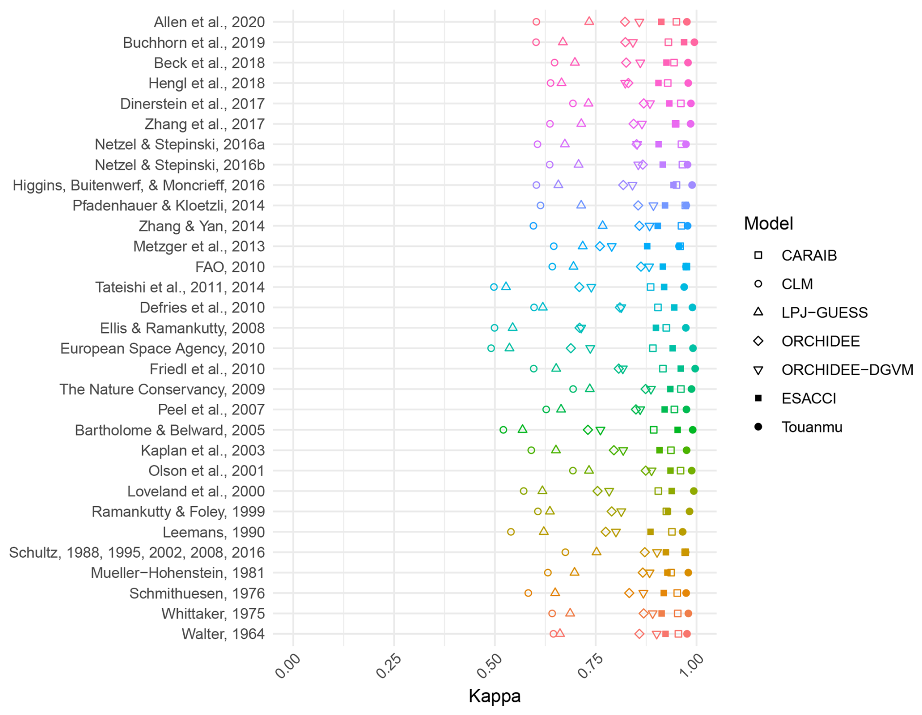
Figure 1 Data-model agreement for different biome maps. For each F31 biome map and each biome map derived from classifying PFTs into biomes, the κ value was calculated. Here, all biomes globally were considered, i.e., κ values were not calculated per biome. Biome classification was conducted with PFT-specific LAI for GVMs and PFT cover for remote sensing products. For the GVMs, simulations for RCP6.0 were used (other RCPs not shown).

Regions where observation-based and modeled biomes agreed or disagreed were spatially heterogeneous (Fig. S5). Agreement was high, for example, in Northern Europe, Northern America, and tropical forest regions in Brazil or Southeast Asia (Fig. S5). Agreement was low on the Tibetan plateau, a large part of the sub-tropics in South America and regions bordering the central African rainforests. Those spatial patterns differed between GVMs and observation-based PFT maps (Fig. S5). For instance, CARAIB showed the highest disagreement in northern latitudes and around the Equator, whereas ORCHIDEE-DGVM showed highest disagreement in sub-tropical regions bordering equatorial forests.

3.2 Biome shifts under climate change

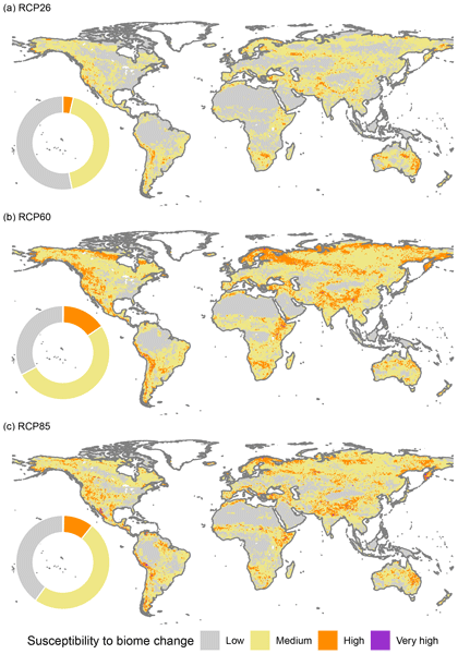
The proportion of grid cells projected to be affected by biome change increased from RCP2.6 to RCP6.0 but was lower in RCP8.5 than in RCP6.0. The RCP8.5 scenario lacks CARAIB and ORCHIDEE-DGVM simulations, the two models with the highest rate of biome shift in other RCP scenarios. In addition to the proportion of grid cells, the susceptibility category, i.e., the number of GVM-biome map combinations that predict biome transitions, increased, indicating higher consensus between different models regarding predicted biome change (Fig. 2). Thus, the area affected by low susceptibility changed from 53.1 % in RCP2.6 to 32.8 % in RCP6.0 and 40.1 % RCP8.5, while the proportion of grid cells affected by high or very high susceptibility increased from 3.6 % in RCP2.6 to 15.5 % in RCP6.0 and 10.7 % in RCP8.5. Yet, the broad spatial patterns of regions affected by biome change were similar for the different RCPs (Fig. 2). For instance, the tropical forests of Africa and Southeast Asia were projected to be stable in all scenarios (grey areas in Fig. 2) while northern latitudes or southern Africa showed a susceptibility to biome changes in all RCPs. The spatial patterns of biome change also differed between GVMs (Fig. S6).

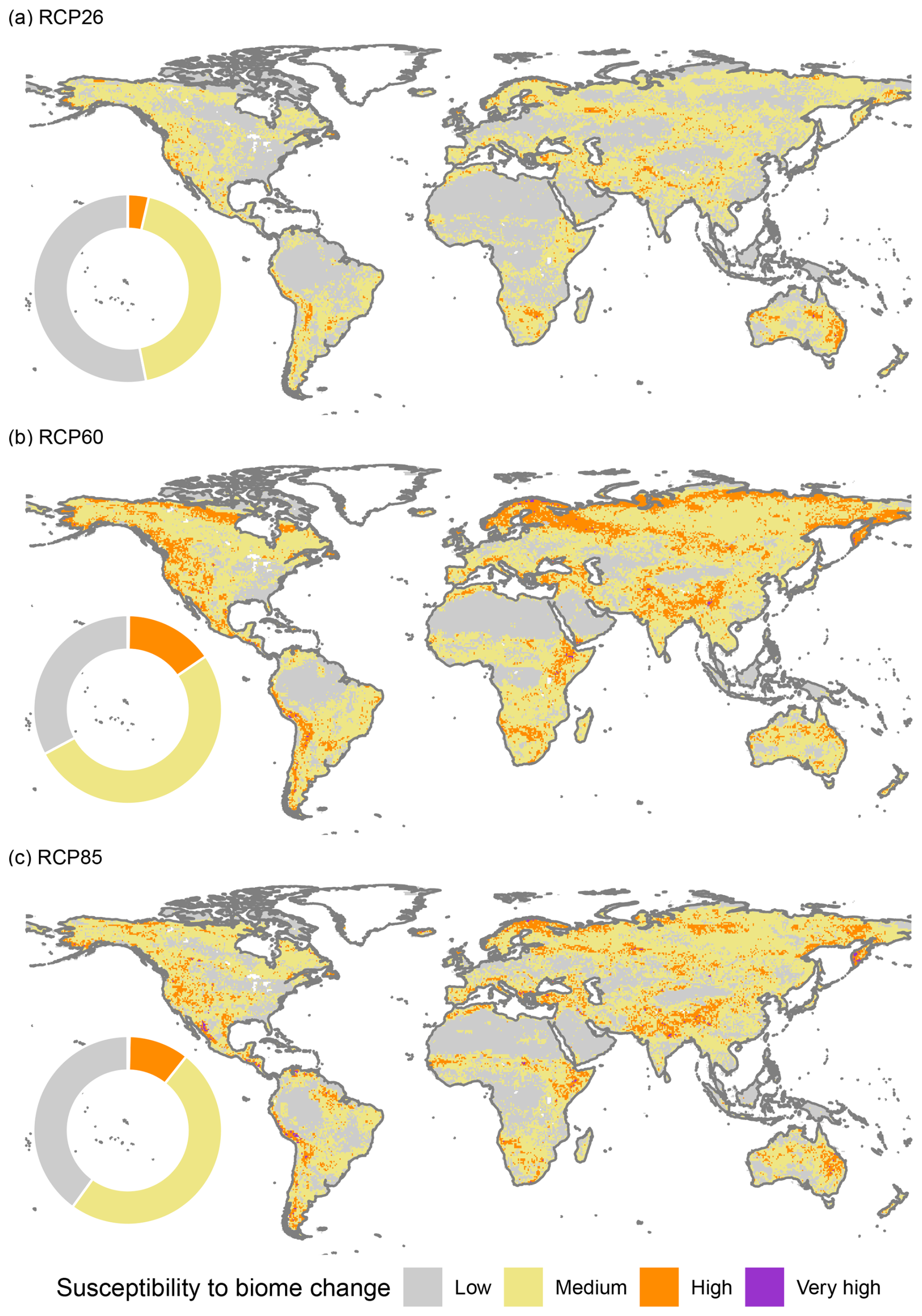
Figure 2 Susceptibility to biome change for different RCP scenarios for all GVMs and all 31 biome maps. The maps show the susceptibility categories derived from the number of models that project a biome change until the end of the century for all combinations of the F31 biome maps and all GVMs available for different RCPs (full ensemble with 403 maps in total). The circle plots indicate the proportion of the land surface in different categories. Susceptibility categories are Low: 0 % to 20 % of the models predict biome shift (i.e., biome stability under climate change); Medium: 20 % to 40 %; High: 40 % to 60 %; Very high: more than 60 %. Note that for RCP2.6 and RCP6.0, 5 different GVMs were available, but only 3 GVMs for RCP8.5. Hence, the categories refer to 155 and 93 biome maps derived from random forest classification.

For all combinations of the GVMs and F31 biome maps, the proportion of the grid cells affected by biome change ranged between 4 %–45 % for RCP2.6 (155 maps), 7 %–56 % for RCP6.0 (155 maps), and 9 %–53 % for RCP8.5 (93 maps, Figs. 3, S7). When averaged across all F31 biome maps for each GVM and each RCP, the proportion of grid cells affected by biome change was lowest for CLM4.5 for all RCPs (4.2 %, 6.6 % and 9.3 %) and highest for CARAIB and ORCHIDEE-DGVM for RCP2.6 (44.5 %), CARAIB for RCP6.0 (56.3 %) and LPJ-GUESS for RCP8.5 (52.7 %, with CARAIB and ORCHIDEE-DGVM not being available for RCP8.5). The proportion of grid cells affected by biome shifts was related to data-model agreement (i.e., the κ value of the respective model, Fig. 3, Table S6). Considering each GVM individually, the proportion decreased when κ is increasing, that is, higher data-model agreement implied a lower rate of biome shifts. When considering all models together, the proportion increased with increasing κ, and the model with the highest overall performance (CARAIB) showed the highest proportion of biome shifts (Figs. 3, S7). These relations were consistent for all RCPs (Fig. S7). The relation between the rate of biome shifts and the number of biomes in the biome map was positive but weak (Figs. 3, S7, Table S7), i.e., more biome types in the biome map imply a higher proportion of biome change. Yet, some biome maps with a lower number of biomes also showed high proportions of biome change.

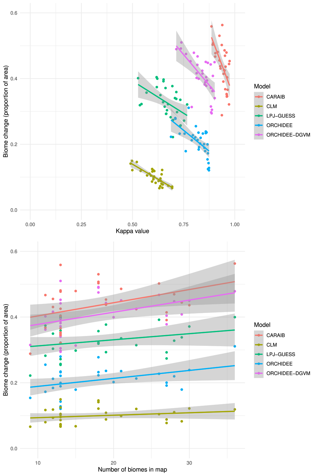
Figure 3 Rate of biome change in relation to data-model agreement and the number of biomes. Each point represents a biome classification for one of the F31 biome maps, and is an average of the entire global-scale results. The κ values were calculated for all biomes in the respective data-model combination. Change represents the proportion of grid cells undergoing biome transitions until the end of the century for a given GVM and biome classification. Figures represent RCP6.0, results for all RCPs are provided in the Supplement.

The regression model showed, that the RCP scenario had a highly significant effect on the number of grid cells affected by biome change (t statistics <0.001, Table S8). The effects of the F31 biome map, GVM and the number of biomes in the map had lower effects, but still significant (t statistics between 0.01 and 0.05). The random forest regression model explained 76.4 % of the variance in the susceptibility to biome change (R²=0.764, RMSE=3.63 %, Fig. 4, Table S9). Temperature anomalies had higher importance than precipitation anomalies. The interaction analysis revealed that temperature sensitivity was significantly higher in the cold zone (temperature <5 °C, p<0.001, Table S10). The partial dependency plots (Fig. S8) revealed a consistent non-linear increase in the susceptibility to biome change with rising temperature anomalies across all climatic zones. The susceptibility saturated at higher temperature increases for all climate zones (Fig. S8). Notably, the cold zone exhibited the highest absolute probability, compared to the temperate and warm zones. In the linear interaction model, the marginal effect of temperature anomalies on the susceptibility to biome change was 1.19 percentage points per °C for the cold zone. In contrast, the sensitivity in warm ecosystems was significantly lower, as indicated by a negative interaction term ($\mathit{\beta }=-\mathrm{0.63},p<\mathrm{0.001}$), resulting in a marginal effect of only 0.55 percentage points per °C.

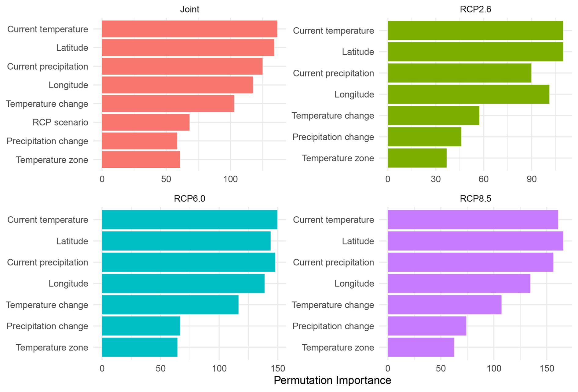
Figure 4 Relative importance of climatic and geographic drivers for susceptibility to biome change. Variable importance was determined using permutation-based importance from random forest models (Combined: R²=0.764; individual RCPs: R²>0.73). “Joint” represents a model where all RCPs were combined.

3.3 Comparison with Olson et al. (2001) biomes

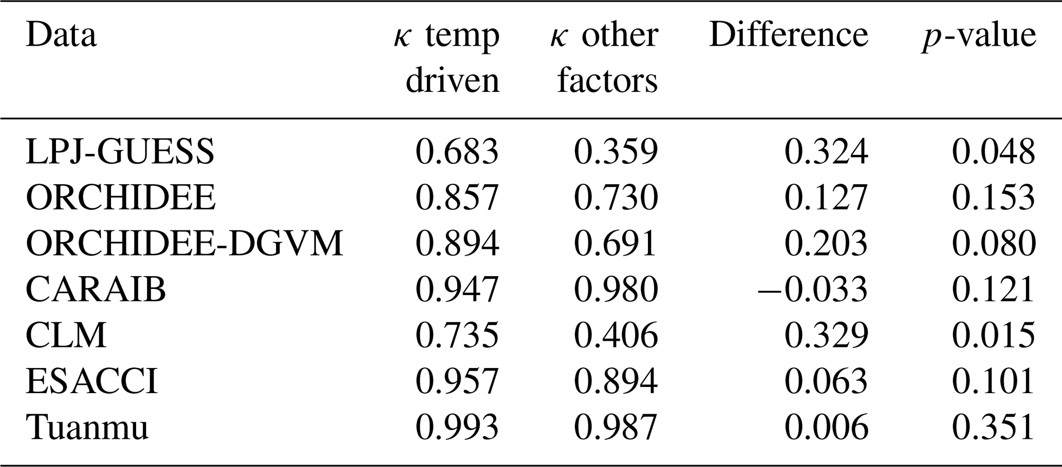
Our biome classification with random forests reproduced the Olson et al. (2001) biome map with high agreement (Fig. S9). The κ value ranged between 0.69 for random forests informed by CLM4.5 and 0.99 for models informed by Tuanmu and Jetz (2014), indicating substantial to almost perfect agreement (Tables S12 to S18). Biome-specific κ varied largely within models and for biomes between different models. For example, the values ranged between 0.40 (moderate agreement) and 0.91 (almost perfect agreement) for different biomes in ORCHIDEE, and between 0.1 (slight agreement) and 0.96 for “flooded grassland and savanna” between different GVMs (and 0.99 for the Tuanmu and Jetz (2014) data). While the proportion of grid cells with data-model disagreement differed between the models, the regions overlapped substantially (Fig. S10). For example, disagreement occurred in areas bordering the central African rainforests, India or the west of North America where temperate conifer forest was not captured by some of the models (Fig. S10). Apart from the CARAIB model, κ values were higher for biomes with biome boundaries controlled by temperature, compared to biomes controlled by other factors (Table 1). Yet, differences were not significant.

Table 1 Performance of random forest models for temperature-limited biomes versus other biomes. The κ was averaged for all biomes in the Olson et al. (2001) biome map that are considered to be mainly limited by temperature or not (i.e., by other factors, see Table S4). Differences between those values were calculated and p-values of t-tests are provided. For the GVMs, only results for RCP6.0 are provided; the results for RCP2.6 and RCP8.5 under current climate are similar (not shown).

The five GVMs projected substantial biome transitions until the end of the century (Fig. 5). The proportion of grid cells where all models projected biome shifts were 0.1 %, 0.3 % and 1.4 % of the land surface for RCP2.6, RCP6.0 and RCP8.5, while the proportion of grid cells not affected by biome change in any model were 51.6 %, 38.7 % and 47.9 % for the RCPs (grey area in Fig. 5). For RCP6.0, the percent of grid cells affected by biome shifts ranged between 6.8 % for CLM4.5 and 37.1 % for CARAIB. The regions affected by biome change did not fully match, but we identified hotspots of potential biome shift. Regions where models consistently simulated biome transitions were scattered across different continents and biomes, for example along the “boreal forest” - “temperate broadleaved mixed forest” biome boundary or in the south of Brazil (Fig. S11). Further, most models projected transitions towards “tropical mixed broadleafed forest” in the regions bordering the central African rainforests, or transitions to “tropical grassland savanna and shrub” in India.

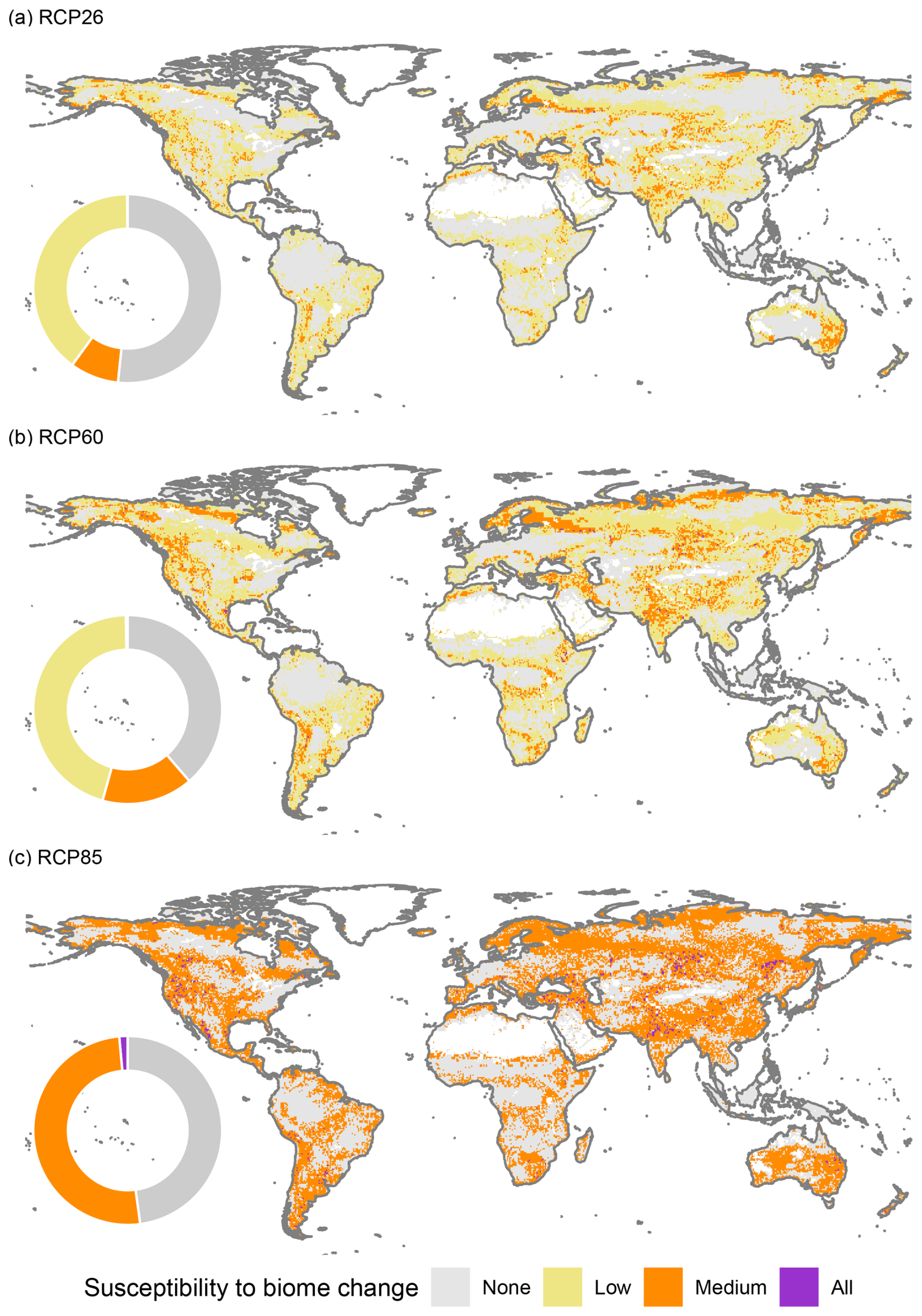
Figure 5 Susceptibility to biome shifts for random forest models informed by the Olson et al. (2001) map. The maps show the number of GVMs projecting a biome shift until the end of the century under different RCPs when biomes were classified using the Olson et al. (2001) biome map (13 maps in total). For RCP2.6 and RCP6.0, 5 GVMs were available, and “Low” and “Medium” indicate agreement of 1 or 2 and 3 or 4 models, respectively. For RCP8.5, 3 different GVMs were available, and “Medium” indicates that 1 or 2 models agree. Category “Low” is not used. Grey areas, e.g., in most tropical forests, indicate biome stability under climate change. For susceptibility maps across all 31 observation-based biome maps see Fig. 2.

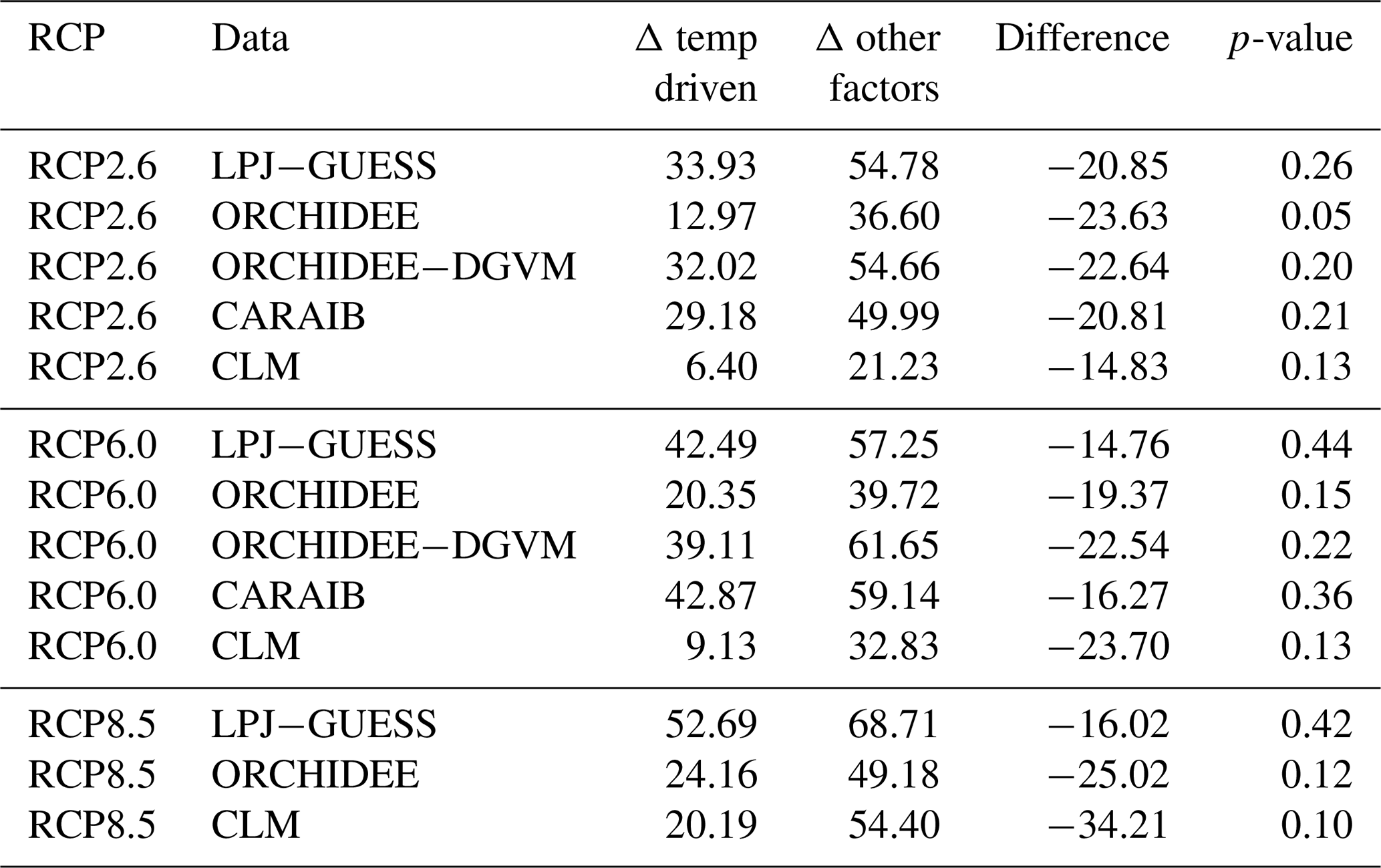
When considering all GVMs and RCPs, the most frequent biome transition was from “tropical and subtropical dry broadleaf forest” to “tropical and subtropical grassland savanna and shrubland” (43.0 %, 52.4 % and 52.9 % of grid cells affected by change for RCP2.6, RCP6.0 and RCP8.5, respectively, Fig. S12). Yet, coverage of “tropical and subtropical dry broadleaf forest” is low under current conditions. When considering only biomes with more than 5 % coverage under current conditions, the most frequent transitions were modeled between “tundra” and “boreal forest/taiga” (18.1 %, 27.8 % and 18.2 % affected, Fig. 6, Table S19). As hypothesized, the analyses showed that biome change was slightly more consistent, i.e., the coefficient of variation of areas affected by specific biome transitions was lower, for temperature-controlled biomes than for other biomes, but not significant (coefficient of variation 0.61 for temperature-driven biomes and 0.68 for others in RCP6.0, p-value 0.522 for t-test comparing coefficients of variation). Yet, the proportion of grid cells affected by change was smaller for temperature-driven biomes (Table 2).

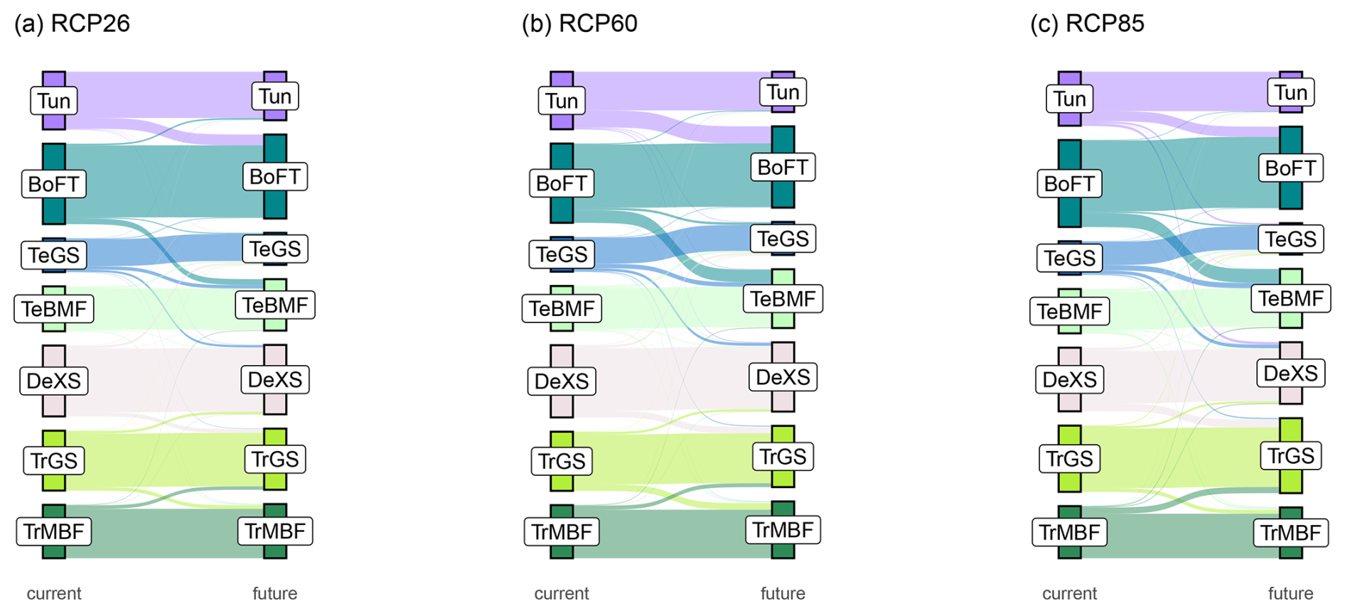
Figure 6 Biome change projected by GVMs for different RCPs. The Sankey diagrams illustrate transitions between different biomes between current and future conditions and biome classification informed by the Olson et al. (2001) map. For each scenario, all available GVMs were included. See Figs. S10, S11 for plots of individual models for RCP6.0. The height of the rectangles represents the biome coverage under current or future conditions, the width of the links represents the number of transitions between biomes. Here, we ignored biomes with low coverage, see Supplement Fig. S12 for graph with all biomes. See Table S11 for full biome names.

Table 2 Biome change for temperature-driven biomes versus other biomes. The proportion of grid cells affected by biome change between current and future conditions was averaged for all biomes in the Olson et al. (2001) biome map that are considered to be mainly limited by temperature or not (i.e., by other factors, see Table S4). Differences between those values were calculated and p-values of t-tests are provided.

4 Discussion

We used LAI simulated by five different GVMs and random forest classification to classify GVM results into biomes of 31 different biome maps (Fischer et al., 2022). In contrast to previous studies using model-specific, expert-based classification schemes, our approach is reproducible and based on multiple biome and land cover maps. This approach facilitates direct comparisons of current and future biome patterns between a large number of model projections. We showed that observation-based biome maps can be reproduced with high agreement, particularly for biomes constrained by well-known temperature limits. Substantial biome changes were modeled with all GVMs for three different RCP scenarios, and the broad spatial patterns of regions susceptible to biome change agreed. Those regions were scattered across all continents. Overall, cold regions showed the highest susceptibility to climate change, and warming had higher effects on susceptibility than precipitation change. The most consistent projection across models and scenarios were poleward shifts of biomes, following temperature increases.

4.1 Biome classification for current conditions

As expected, random forest models using GVM results and observation-based PFT maps showed high performance and agreement with the F31 biome maps (high κ value). The performance of RFs using PFT maps was higher than those using GVM results. This result is not surprising as PFT maps were derived from various remote sensing products (Tuanmu and Jetz, 2014; Harper et al., 2023), and they are therefore not fully independent from biome maps derived from similar remote sensing products (Fischer et al., 2022). It is more remarkable that biome maps derived from GVM results showed very high agreement with observation-based biome maps (κ>0.8) for some combinations of GVM and the F31 biome maps. GVMs are process-based and bottom-up (Prentice et al., 2007), and biome information is typically not directly used to parameterize such models. Yet, some models constrain current and future PFT cover fractions (e.g., CLM4.5) using observation-based PFT or biome data, instead of simulating PFT cover dynamically (e.g., LPJ-GUESS). However, LPJ-GUESS and other models use bioclimatic limits to constrain the distribution of PFTs, and these constraints also influence the possible distributions of biomes defined by those PFTs. Bioclimatic limits and responses to climate change differ between models. For example LPJ-GUESS, ORCHIDEE-DGVM, ORCHIDEE, and CLM4.5 mainly use temperature-based bioclimatic limits to constrain PFTs, whereas CARAIB adds explicit drougth tolerance constraints (Tables S2 and S3).

For GVMs, κ values were highest for the Schultz (2016) biome map. Classification in this map is based on vegetation, climate and other environmental factors, and re-evaluation of previous, regional-scale studies. The Schultz (2016) map shows a clear arrangement of biomes along environmental gradients and the relation to climatic drivers. High agreement with GVM results illustrates that biomes simulated by GVMs reflect the prevailing climatic conditions and bioclimatic limits that constrain the distribution of PFTs. Similarly, agreement between GVMs and the Olson et al. (2001) map, a map derived from species distributions and biogeographic zonation, was high. The Olson et al. (2001) map has often been used as reference map in biome-specific studies, for example, of the human footprint (Sanderson et al., 2002), climate change velocity (Loarie et al., 2009), or biodiversity intactness (Newbold et al., 2016). High agreement confirms that the Olson et al. (2001) biome map is suitable as a reference for such analyses.

Agreement between observation-based and modeled biomes was spatially heterogeneous. For example, in the Olson et al. (2001) map, agreement was lowest on the Tibetan plateau. Olson et al. (2001) also used elevation to define biomes, which is not used by the GVMs to simulate biomes. Other regions with low agreement were the sub-tropics surrounding the central African rainforests. It has been hypothesized, that in some of these regions, alternative biome states are possible (Pausas and Bond, 2020), that is, depending on fire activity or herbivores, closed forests or open savanna states are possible (Higgins and Scheiter, 2012; Midgley and Bond, 2015). Fire has been included in many GVMs (Hantson et al., 2016), including the models in our study, and shown to influence modeled tree cover and the carbon cycle (Lasslop et al., 2020). If fire enables alternative states and influences biome patterns in our results remains to be tested. Nevertheless, our study identified data-model mismatches for different GVMs and can be used to identify model limitations or to attribute uncertainties to fire, animals, humans or other factors. Doing such detailed analyses for the different models is, however, beyond the scope of our study.

Despite the large variation between different combinations of GVMs and F31 biome maps, κ values were overall higher than in previous studies. For instance, Dallmeyer et al. (2019) reports values between 0.2 and 0.79 in a comparison between different models and classification methods, and Scheiter et al. (2024a) reports a maximum value of κ=0.52 for a classification using functional traits modeled by the aDGVM2. This can be attributed to the application of random forest classification that often shows high performance (Fernandez-Delgado et al., 2014), while previous GVM studies typically applied expert-based biome classification approaches. Random forests maximize the agreement between modeled and observation-based biomes at the expense of clear and justifiable rules to separate between biomes. Further, we created a large ensemble of biome maps with κ values ranging between around 0.5 and >0.95.

4.2 Biome shifts under climate change

All GVMs projected biome shifts until the end of the century, irrespective of the Fischer et al. (2022) biome map used to inform the biome classification. Yet, the proportion of grid cells affected by biome change varied between different RCPs, GVMs and biome maps. Across all RCPs and GVMs, regions with high susceptibility of biome change were distributed across all continents, for example in southern Africa, the northern latitudes of Eurasia, or south of the Amazon rainforests. Biome stability or low susceptibility of biome change was consistently modeled in deserts and tropical rainforests globally.

Our results confirm some previous modeling results. In a global study, Gonzalez et al. (2010) also identified deserts and tropical forests as biomes with lowest susceptibility of biome change and higher susceptibility in the northern latitudes. Huntley et al. (2016) showed with LPJ-GUESS simulations that a large proportion of desert and rainforest have also been stable during the last 140 ka, showing their stability under past, current and future conditions (at least without direct human impacts). Yet, Parry et al. (2022) found that five out of seven climate-vegetation models project Amazon forest dieback at the local scale, that may, however, be compensated by increases in carbon elsewhere at larger scale. Doughty et al. (2023) argued that under future warming, tropical forests may approach ecophysiological limits that inhibit further growth, particularly under RCP6.0 and RCP8.5. In combination with deforestation, warming may lead to tipping point behavior and transitions into degraded states (Wunderling et al., 2026). However, such effects may be compensated by adaptation and acclimation of temperature optima (Choury et al., 2022), or by high functional diversity buffing drought effects (Langan et al., 2025). Amazon forests may also experience more hot droughts and non-analogue climate under future conditions, enhancing the risk of forest dieback (Chambers et al., 2025). Such large-scale die-back is not confirmed by our results and susceptibility to biome change was only low to moderate in the Eastern parts of the Amazon. The reasons for this discrepancy to other studies is not clear but likely related to different climate forcing data or to CO₂ fertilization that may overcompensate precipitation change in the GVMs. Such compensation effects have been observed, for example for Eucalyptus species grown in pots (Jiang et al., 2021).

Biomes in the cold zone were generally more susceptible to warming than other zones. Our results for the Olson et al. (2001) biome map revealed that “temperate grassland savanna and shrubland” and “tundra” were highly susceptible to biome shifts in all RCPs. This result partly agrees with Gonzalez et al. (2010), who identified temperate mixed forests, boreal conifer forests, and tundra/alpine as most vulnerable to biome shifts. Similarly, Tobian et al. (2024) showed with the LPJmL model that boreal forests are highly susceptible to dieback while temperate forests are relatively resilient and tropical forests are relatively stable.

While thermal acclimation and adaptation of temperature optima could mitigate some warming impacts (Choury et al., 2022), these processes are often not well represented in current GVMs. They often rely on fixed thermal response functions (Wang et al., 2025) to model for example photosynthesis and respiration. Consequently, the lack of dynamic acclimation in models may lead to uncertainty in predicting the resilience of ecosystems under climate change (Wang et al., 2024). Ecopysiological processes and bioclimatic limits drive the performance of different PFTs at different temperatures. For instance, at low temperatures bioclimatic limits may constrain establishment of a specific PFT and unusual extreme cold can also kill trees, while at high temperatures respiration may reduce productivity. Climate change therefore has PFT-specific effects on the productivity, LAI, spatial coverage, and may thereby trigger biome transitions. In GVMs, the climatic niche of PFTs is generally preserved, and novel climates do not imply acclimation and adaptation. Whether novel and non-analogue biome states, characterized by novel combinations of PFT composition emerge in GVMs, remains to be tested. Uncertainties persist regarding the extent to which CO₂ fertilization offsets physiological stressors (Walker et al., 2021) in emerging environmental niches and the models' ability to capture extreme heat and drought remains a key challenge for model development.

One reason for discrepancies between our and previous results is that predicted future large-scale dieback events are climate- and vegetation-model-specific (e.g., Sitch et al., 2008; Rammig et al., 2010). For example, in LPJ-GUESS in this study the high-temperature stress function for boreal trees that LPJmL includes (Tobian et al., 2024) has been deleted more than ten years ago because the developers concluded that there is not enough observational data to parameterize this function. Therefore, LPJ-GUESS does not predict heat-related mortality and dieback in the boreal forest. Which model combination is most realistic is, at present, impossible to say, partly because it has hardly been tested to what extent the current GVMs can reproduce recent increases in drought- and heat-related tree mortality and extreme fires (Steinkamp and Hickler, 2015), such as the record fires in Canada in 2023 (MacCarthy et al., 2024). Data-model comparisons for the recent sharp increase in drought-induced mortality of Norway spruce in Central Europe, in some regions reaching 50 % of the forest area, have shown that most GVMs fail to reproduce the observed large-scale forest die-back (Anders et al., 2025; Fischer et al., 2025). Thus, the current GVMs might underestimate future risks of climate-induced forest dieback and associated biome shifts, but more studies will be necessary to corroborate such a conclusion. Given the limitations of the representation of tree mortality in vegetation models (Langan et al., 2025; Scheiter et al., 2024b; Anders et al., 2025), improving the mortality in vegetation models will not only improve the representation of current ecosystem dynamics and biome boundaries, but also reduce uncertainties in projections of future climate change effects.

Our findings demonstrate that biome stability and biome shifts are primarily driven by temperature forcing, i.e., current temperature and temperature change. The higher sensitivity of biomes in the cold zone to warming suggests that these regions are approaching critical ecological thresholds. The saturation effect in the susceptibility to biome shifts beyond approximately 4 °C in the cold zone and 7 °C in the temperate and warm zone indicates a state of maximum climate-driven biome change that was reached at lower temperature change in the cold zone. These results underscore that vulnerability of biomes in the cold zone is not merely a function of higher warming under climate change but is caused by the higher intrinsic sensitivity of ecosystems to warming. In contrast to the tropics, acclimation may not necessarily buffer vulnerability to warming in cold and high-altitude biomes. Recent evidence suggests that alpine species possess a more limited capacity for thermal acclimation compared to other biomes (Harris et al., 2024).

For each GVM, the proportion of grid cells affected by future biome change decreased as data-model agreement (the κ value) with one of the 31 biome maps (Fischer et al., 2022) increased, i.e., higher agreement implies a lower proportion of grid cells affected by biome change. A similar relation was found in Scheiter et al. (2024a) for the classification of aDGVM2 results into biomes using PFT cover fractions or patterns of functional traits modeled by the aDGVM2 (Scheiter et al., 2013; Langan et al., 2025). This result suggests that the rate of projected biome shifts may be overestimated when a biome classification with low data-model agreement is used. In contrast, biome classifications with high agreement may provide an estimate of the minimum rate of biome change, and potentially a more reliable trend of biome change. For RCP6.0, this lower limit is between 21.9 % and 28.9 % for the different GVMs.

Interestingly, assessing this relation across all GVMs included in our analysis showed the opposite, i.e., an increasing proportion of grid cells affected by biome change with higher data-model agreement. For better performing GVMs (i.e., higher κ) the random forest is more precisely defined and therefore more sensitive to LAI changes. Biome maps with low performance (i.e., poorer κ values) reflect weaker compatibility with the model PFTs, leading to spurious relationships and reduced sensitivity of the random forest models to LAI changes. CARAIB has the highest number of PFTs and the highest number of grid cells affected by biome change. A biome type may, in our classification, be represented by multiple PFTs, and moderate LAI changes of multiple PFTs may translate into a biome change. In models with a low number of PFTs, such as CLM4.5, a biome can be represented by a single PFT, and substantial changes in LAI may be required to trigger a biome change. In addition, PFT cover fractions in CLM4.5 remain static under future climates, such that biome change is constrained and only driven by LAI change.

4.3 Biome shifts of temperature-driven biomes

Our results for the Olson et al. (2001) map support the hypothesis that biomes with well-described temperature limits, including for example tundra and boreal forest (Table S4), are better reproduced by the random forest models than biomes driven by other factors. Yet, differences between κ values of those groups of biomes were not statistically significant. Many GVMs include bioclimatic limits related to temperature to constrain the distribution of different PFTs (e.g., Sitch et al., 2003, Table S3 for GVMs included in the study). These limits describe, for example, cold tolerance or chilling requirements of PFTs, and they are based on empirical evidences (Prentice et al., 1992). Given the constraints on PFTs, bioclimatic limits also constrain the distribution of biomes. Yet, single PFTs do not match directly with biomes. Hence, it is not a priori clear, that GVMs using bioclimatic limits and ecosystem dynamics represented in GVMs will produce LAI and PFT patterns that represent the biomes included in different biome products. We therefore conclude that bioclimatic limits alone do not explain the good data-model agreement in our study. Thus, the border between forests and tropical and temperate grasslands is in most models not defined by bioclimatic limits and instead emerges from the competition between grasses and trees in interaction with fires.

Temperature-driven biomes showed lower proportions of grid cells affected by biome shifts than those controlled mainly by other factors. Yet, as expected, biome transitions were slightly more consistent for temperature-driven biomes (not statistically significant), i.e., the variability of possible future biome types for a given biome type under current conditions was lower between different models. This could be attributed to the representation of PFTs and bioclimatic limits in the models, but also to spatial patterns of changes in environmental conditions. Temperature is less variable among the climate models than other variables such as precipitation or aridity, and temperature changes are mainly directed poleward, in contrast to other variables (Shi et al., 2021). In the GVMs, temperature increases and elevated CO₂ in different RCP scenarios do not only modify ecophysiological processes, the carbon balance and competitive hierarchies of PFTs but temperature change may also imply that bioclimatic limits of PFTs are crossed (Tables S2, S3). Hence, climatic conditions may become unsuitable for the PFT, which implies poleward biome shifts, following the warming trends in the RCP scenarios. Changes in biomes that are not mainly driven by temperature indicate that effects of other variables such as change in rainfall regimes, CO₂ or fire activity have stronger effects on those biomes than change in temperature. Fire is included in many GVMs (Hantson et al., 2016), including models used in our study. A recent analysis highlights the model's applicability for burned area attribution (Burton et al., 2024) and further model comparisons focusing on fire are ongoing (Burton et al., 2025). Yet, we did not analyze fire effects on biome change.

4.4 Limitations and future directions

The LPJ-GUESS version used in this study and some of the F31 biome maps (e.g., Olson et al., 2001) only include natural vegetation, while other GVMs and biome maps also include cultivated areas. For consistency, we used only PFTs and biomes representing potential natural vegetation. Yet, direct human impacts such as deforestation of Amazon rainforests or intense livestock grazing in savannas have shaped the current biome distribution and can accelerate or inhibit biome change in the future (Scheiter and Savadogo, 2016). While land use, nitrogen deposition and fertilizer input were considered but fixed at year 2005 levels in our analysis, it could be repeated by including PFTs and biomes representing cultivated land and by using available ISIMIP results simulated with changes in land use, nitrogen deposition and fertilizer input according to HYDE3.2 for historic conditions (Klein Goldewijk et al., 2017) and to MAgPIE simulations for SSP2 for future conditions (Popp et al., 2014; Stevanović et al., 2016). Considering only potential natural vegetation is, however, important for conservation and protection of the remaining natural vegetation.

We used LAI simulated by different GVMs for biome classification, for consistency with biome classification schemes used in previous modeling studies (e.g.,  Smith et al., 2014). LAI is directly modeled by GVM, observable and it has direct biophysical meaning. Hence, our approach provides a functional description of biomes, based on productivity and relative abundance of different PFTs. Selection of appropriate variables for biome classification is not only relevant for model results but also for observation-based biome maps. Depending on the variables used for classification and the number of biome types represented, the resulting biome maps can vary substantially (Beierkuhnlein and Fischer, 2021; Fischer et al., 2022). The F31 biome maps span six decades and various mapping approaches, from pre-satellite expert-based maps to modern products that integrate satellite remote sensing products. Direct comparisons of their agreement would require harmonization and re-classification (Dallmeyer et al., 2019; Champreux et al., 2024). Our approach sidesteps such re-classification, by creating a random forest model for each F31 biome map.

While our random forest classification approach is reproducible and can be applied to any GVM, it has a major caveat: rules for classification are less transparent than in expert-based biome schemes tailored for specific GVMs and biome types. Yet, identifying thresholds to delineate between biomes using quantitative methods or expert knowledge has their own flaws. We therefore argue that large-scale model comparisons benefit from utilizing reproducible classification methods that can be applied to any set of PFTs included in GVMs. Expert-based classification schemes are more applicable for studies with single GVMs.

Vegetation change has been shown to lag behind change in environmental forcings (e.g., Bertrand et al., 2016; Scheiter et al., 2020; Zani et al., 2024). Hence, vegetation and biome patterns are committed to further change to reach an equilibrium state with climate, even if the climate system stabilizes. These lags can be explained by various processes including dispersal limitation, delayed responses of ecological processes such as ecophysiology, establishment and mortality, succession, and disturbances such as drought or fire. Dispersal has been integrated into GVMs (e.g., Blanco et al., 2014; Zani et al., 2022). Yet, consideration at global scale is challenging as dispersal is strongly influenced by small-scale processes and heterogeneity that cannot be represented at the 0.5° resolution of the GVM simulations (Lenormand et al., 2009; Snell et al., 2014). In our analysis, we ignored potential biome shifts between the publication of the different observation-based biome maps (Fischer et al., 2022) and our reference period for the analyses, and respective temporal mismatches or lag effects. Nonetheless, random forests based on GVM results reproduced broad biogeographic patters encoded in the different observation-based biome maps.

5 Conclusions

We present a reproducible biome classification approach that can be applied to any GVM and observation-based biome map, and that allows multi-model comparisons of climate change impacts on future biome distributions. We showed that substantial biome shifts are likely under future climate change scenarios. The most susceptible regions differ between GVMs, RCP scenarios and biome maps used to inform biome classification, highlighting the need for multi-model analyses. Despite these differences, we identified consistent patterns, including poleward shifts of biomes, primarily in response to temperature increases in the cold zone, as well as stability in desert and equatorial rainforest regions. This contrasts several previous studies that predicted widespread dieback of boreal and tropical forest. The ranges of the proportion of grid cells affected by future biome shifts ranged between 4 % and 56 % for all models and RCPs considered in this study (403 maps in total). Even in the low-emission scenario RCP2.6, biome changes were modeled and some regions are expected to experience low or even high susceptibility of biome change. Such change in the global distribution of biomes may imply substantial implications for biodiversity and ecosystem services and functions and thereby have strong impacts on human societies (Parmesan et al., 2022). Our study can help identifying biomes and regions where biodiversity conservation, adapted land management, and climate policy are most urgent.