The open uncertainty window in ocean biogeochemical responses to fossil carbon emissions

Automated parameter optimisation can effectively reduce model-data mismatch and provide information about ocean biogeochemistry parameter sensitivities, but to what extent it reduces uncertainty in responses to climate change is not well understood. To explore the robustness of simulated ocean biogeochemical responses to a “business-as-usual” RCP 8.5-equivalent fossil CO₂ emission scenario until year 2300, six biogeochemical parameters are optimised against contemporary oxygen, phosphate, and nitrate fields in three different physical configurations of the UVic ESCM. The phytoplankton maximum growth rate parameter value and the nitrogen-to-oxygen molar ratio of organic matter remineralisation were found to be robust across the calibration ensemble, with the former varying less than 1.6 % across the calibrated ensemble and the latter varying less than 4 %. While each calibrated model performs nearly equivalently in terms of optimal total misfit (a result of the model calibration objective), significant differences in biogeochemical fluxes and rates (e.g., global net primary and particulate organic carbon; POC) remain. Application of CO₂ emissions to the calibrated models to the year 2300 produces model responses that start diverging in global average trends in the early 2000s. Models with more sluggish pre-industrial circulations respond less to climate warming in terms of physical changes, but more in their primary production (as these models have been tuned to have weaker limitation on production). Models that have larger changes in circulation metrics due to anthropogenic CO₂ emissions, in particular the Southern Ocean overturning, demonstrate larger changes in shallow (130 m) and deep (2 km) POC fluxes (due to stronger parametric control on particle flux). Suboxic volume trends are smaller in models with larger changes to the physical circulation metrics owing to compensation between model tuning favouring strong biological oxygen consumption in their vigorous pre-industrial state and these models' having a greater physical sensitivity to warming. By the year 2300, the resulting model responses vary by a factor 2.8 in net primary production, 5 in shallow POC fluxes, 1.7 in deep POC fluxes, 1.5 in nitrogen fixation and 1.2 in suboxic volume, but the model spread in absolute values relative to the pre-industrial remains largely unchanged, demonstrating the utility of constraining the pre-industrial ocean state in diverse model ensembles for robust projections of ocean change. However, an uncertainty window remains open in ocean biogeochemical responses to CO₂ emissions, despite systematic tuning.

1 Introduction

Parameter choice for global biogeochemical models is a critical step in model development, as different biogeochemical parameter values will produce different pre-industrial states when integrated over thousands of years (e.g., Kriest et al., 2010, 2012; Kwon et al., 2009). Differences in the distribution of oxygen and dissolved inorganic carbon (DIC) arising from parameter choice can be the same order of magnitude as those induced by physical differences in the circulation (Najjar et al., 2007). Biogeochemical models can be calibrated using optimisation techniques to obtain similar misfits against observations such as gridded nutrients (Kriest, 2017; Kriest et al., 2017, 2020, 2023), but with large resulting differences in nutrient pathways (Yao et al., 2019) and biogeochemical fluxes (Kriest et al., 2023). Which biogeochemical parameter values may be considered optimal depends both on the metric applied to assess the misfit (Sauerland et al., 2019; Evans, 2003) and on the large-scale features of the model general circulation that is used for the optimisation (Kriest et al., 2020).

There are few studies of how biogeochemical parameter differences affect transient projections such as under anthropogenic CO₂ emissions. This is because Earth system and ocean models typically vary not only in terms of their biogeochemical parameters but also their physical set-up (e.g. Cocco et al., 2013; Cabré et al., 2015), as well as in how they are spun up (Séférian et al., 2016), how long they are spun up (Kriest et al., 2023), or in their pre-industrial ocean mean state (Ödalen et al., 2018). However, it has been shown that biogeochemical models that perform similarly against contemporary nutrient distributions may diverge under transient forcing with respect to their net primary and export production (Kvale and Meissner, 2017), the development of suboxia (Löptien and Dietze, 2017; Löptien et al., 2021), and the response of the biological carbon pump to warming (Pasquier et al., 2023). Yao et al. (2022) demonstrated that biogeochemical models performing similarly with respect to global oxygen and nutrient distributions in pre-industrial steady-state (Yao et al., 2019) can produce nitrogen cycle trends (global denitrification and nitrogen fixation) of opposite sign with climate warming. At the same time, relatively small differences in ocean vertical mixing parametrisation have been demonstrated to influence ocean heat and carbon uptake in transient scenarios in one Earth system model (Ehlert et al., 2017). Physical parameters related to circulation and anthropogenic carbon uptake (e.g. Mignone et al., 2006) have been studied for decades, but testing their impact on simulated ecology, nutrient and oxygen distributions under transient conditions is still relatively new (e.g. Bahl et al., 2019). A recent study by Pasquier et al. (2023) found that a biogeochemical model calibrated for two different ocean circulations, with similar resulting steady-state biological pump strengths (measured by the fraction of the global phosphate inventory that is regenerated), produced substantially differing carbon and oxygen cycle responses to forcing. Taken together, this body of work demonstrates a high level of parametric and structural uncertainty inherent in Earth system and ocean biogeochemical models and their projections of future ocean biogeochemical cycling, and the ecosystem services these cycles provide. Only systematic testing of model parameter space with respect to physical and biogeochemical parameters can offer insight with respect to transient model uncertainties, and how they might evolve with anthropogenic climate forcing.

Our manuscript addresses two objectives. The first objective is to define a window of model uncertainty for projections of marine biogeochemical cycling under climate change, based on a set of equally-likely biogeochemical parameter value combinations for different vertical mixing parametrisations. The second objective is to quantify correlations in circulation metrics with biogeochemical metrics for a contemporary ocean and to estimate their relevance for predicting long-timescale ocean biogeochemical change. We do this by systematically exploring biogeochemical model sensitivity to vertical mixing parametrisation and biogeochemical parameter choice in an Earth system model, using a work flow shown in Fig. 1. We use a combination of classical, fully-coupled online model simulations as well as an offline framework (Kvale et al., 2017). The offline framework exploits the computational efficiency provided by the Transport Matrix Method (TMM) (Khatiwala et al., 2005; Khatiwala, 2007). The TMM is a method to spin-up ocean circulation models 100 times faster than is normally required in a fully-coupled framework. Fast spin-ups allow us to calibrate biogeochemical parameters in the ocean model using a search algorithm and global misfit cost function to fit the model to observational data (Kriest et al., 2017; Kriest, 2017). The offline calibration framework has been adapted to the University of Victoria Earth System Climate Model (UVic ESCM Weaver et al., 2001; Eby et al., 2009; Yao et al., 2019). The parameters of three vertical mixing schemes are tuned to achieve as-similar-as-possible overturning circulation strengths in the online configuration, and their transport matrices are extracted to carry out the offline biogeochemical parameter optimisation. The mixing-specific biogeochemical parameters are then applied in the fully-coupled online Earth system model to test for resulting systemic sensitivity in carbon and nutrient cycling. All data and model setup code used to produce the parameter calibrations as well as the online transient simulations are provided in the GEOMAR repository (Kvale et al., 2021).

Figure 1 Work flow used in the model set-up and simulations. CON, TID, and BL stand for constant, tidal, and Bryan-Lewis vertical mixing schemes, respectively.

2 Methods

2.1 Modelling framework

The University of Victoria Earth System Climate Model (UVic ESCM) version 2.9 (Weaver et al., 2001; Meissner et al., 2003; Eby et al., 2009) is an intermediate-complexity Earth system model with a resolution of 3.6° by 1.8° and 19 vertical ocean depth levels. It contains an ocean model, land and vegetation components, a dynamic-thermodynamic sea ice model, and sediments. The atmosphere is represented by a two-dimensional energy-moisture balance model. Winds are prescribed from monthly NCAR/NCEP reanalysis data (Weaver et al., 2001). Continental ice sheets are fixed. The biogeochemical module (UVOK) is a nutrients-phytoplankton-zooplankton-detritus (NPZD) model that contains two classes of phytoplankton (ordinary phytoplankton and nitrogen-fixing diazotrophs), a single zooplankton class, and inorganic tracer representation of nitrate, phosphate, oxygen, dissolved inorganic carbon (DIC), and alkalinity. Water column denitrification is simulated but benthic denitrification is not. Keller et al. (2012) updated the parametrisation of grazing and added iron limitation to the phytoplankton growth equations based upon the seasonal model outputs of the global biogeochemistry model BLING (Galbraith et al., 2010). Kvale et al. (2017) separated the UVic ESCM version 2.9 biogeochemistry into the stand-alone UVOK module and introduced a Transport Matrix Method (TMM) (Khatiwala et al., 2005; Khatiwala, 2007) interface.

The TMM is an efficient, matrix-based simulation scheme for ocean biogeochemical tracers (Khatiwala et al., 2005; Khatiwala, 2007). It allows the offline computation of seasonally cycling, steady-state solutions by applying the biogeochemical equations to a sparse matrix of physical tracer tendencies which encapsulate the model steady-state circulation. Furthermore, it is massively parallel (the online UVic ESCM is serial code), which reduces equilibration times from weeks to hours when integrated on sufficiently large high performance computing machines (Kvale et al., 2017). The TMM's computational efficiency enables the systematic testing of biogeochemical model parameter space, including model calibration and parameter optimisation against various metrics.

Kriest et al. (2017) introduced an estimation of distribution algorithm (the covariance matrix adaptation evolution strategy; CMA-ES, (Hansen and Ostermeier, 2001)) to the TMM framework. The CMA-ES framework defines for each iteration (that is, “generation”) a population of 10 individual parameter value combinations that are selected from within a prescribed parameter value probability distribution. These 10 parameter combinations are integrated in the TMM for 3000 years to achieve approximate model steady-state, at the end of which a misfit function (the root-mean-square-error, RMSE) is evaluated against annual-mean gridded observations of modern ocean phosphate (j=1), nitrate (j=2), and oxygen (j=3) (Garcia et al., 2010a, b). The misfit is weighted by the volume V_i of each individual grid cell and is expressed as a fraction of total ocean volume V_T. Each individual component (j) is normalised by the global mean concentration of the observed tracer ($\overline{o_j}$) for summation. The misfit function (J) is thus:

$$\begin{array}{}\text{(1)}& J=\sum _{j=\mathrm{1}}^{\mathrm{3}}{\displaystyle \frac{\mathrm{1}}{\overline{o_j}}}\sqrt{\sum _{i=\mathrm{1}}^N(m_{i,j}-o_{i,j}{)}^{\mathrm{2}}{\displaystyle \frac{V_{\mathrm{i}}}{V_{\mathrm{T}}}}}.\end{array}$$

Here, N is the number of model grid cells (87 307 in the UVic ESCM) and m_i,j and o_i,j are modelled and observed tracer concentrations, respectively. Results of the evaluation, as well as those of the previous generations, inform a revision of the parameter value probability distribution for the next generation. Thus, the algorithm reduces misfit until an optimal parameter combination that minimizes the misfit is achieved (typically, 70–150 generations in our particular framework and model). Testing suggests the framework is limited to calibration of about 6 parameters simultaneously; more than that prevents the misfit from converging to a minimum solution.

2.2 Vertical mixing parametrisation

Similar to Ehlert et al. (2017), the UVic ESCM version 2.9 (Eby et al., 2009) is equilibrated using pre-industrial (year 1776) atmospheric CO₂ boundary conditions of 278 ppm, and 3 commonly used vertical mixing schemes: the default scheme, Bryan-Lewis (BL) (Bryan and Lewis, 1979), spatially constant (CON), and a tidally-driven mixing scheme (TID) (Schmittner et al., 2005). BL vertical mixing utilises a diffusivity parameter that increases with depth but is laterally constant (Weaver et al., 2001). CON vertical mixing uses a scalar diffusivity parameter (both laterally and depth-independent). TID mixing adds topographically dissipated tidal energy to the constant diffusivity parametrisation in order to mimic lateral and depth variability in tidally-driven mixing, where a stability dependency permits the diffusivity to evolve with the model state (in a fully-coupled online implementation) (Schmittner et al., 2005). All are hand-tuned to an average Northern Hemisphere maximum meridional overturning strength of 17.5 Sverdrups (within the middle of the range provided in Cunningham et al. (2007)); work flow step A in Fig. 1. The tuning was done by adjusting the scalar vertical diffusivity parameter (k_v) in TID and CON, or parameter scaling (in the case of BL), until the desired overturning strength was achieved. The parameter scaling in BL preserves the slope of change between surface and seafloor vertical diffusivity, where the default configuration used a k_v between 0.3 and 1.3 cm² s⁻¹. Resulting vertical diffusivity values and a selection of biogeochemistry-relevant physical diagnostics (Kriest et al., 2020) used in our analysis are given in Table 1, and the vertical diffusivity is plotted by ocean basin in Fig. 2. Numerical ocean circulation models typically use observationally-informed k_v values within a range of 0.01 to 0.5 cm² s⁻¹ (Duteil and Oschlies, 2011), so our model values are on the higher end of this range. All other physical parameters are the same across configurations. These three different models are produced to test the impact of vertical mixing parametrisation on biogeochemical parameter optimisation, while seeking to minimise the impact of variable meridional overturning. Models were integrated to steady-state over 10 000 years (work flow step B in Fig. 1). Transport matrices were then extracted from the models using methods described by Kvale et al. (2017) (work flow step C in Fig. 1).

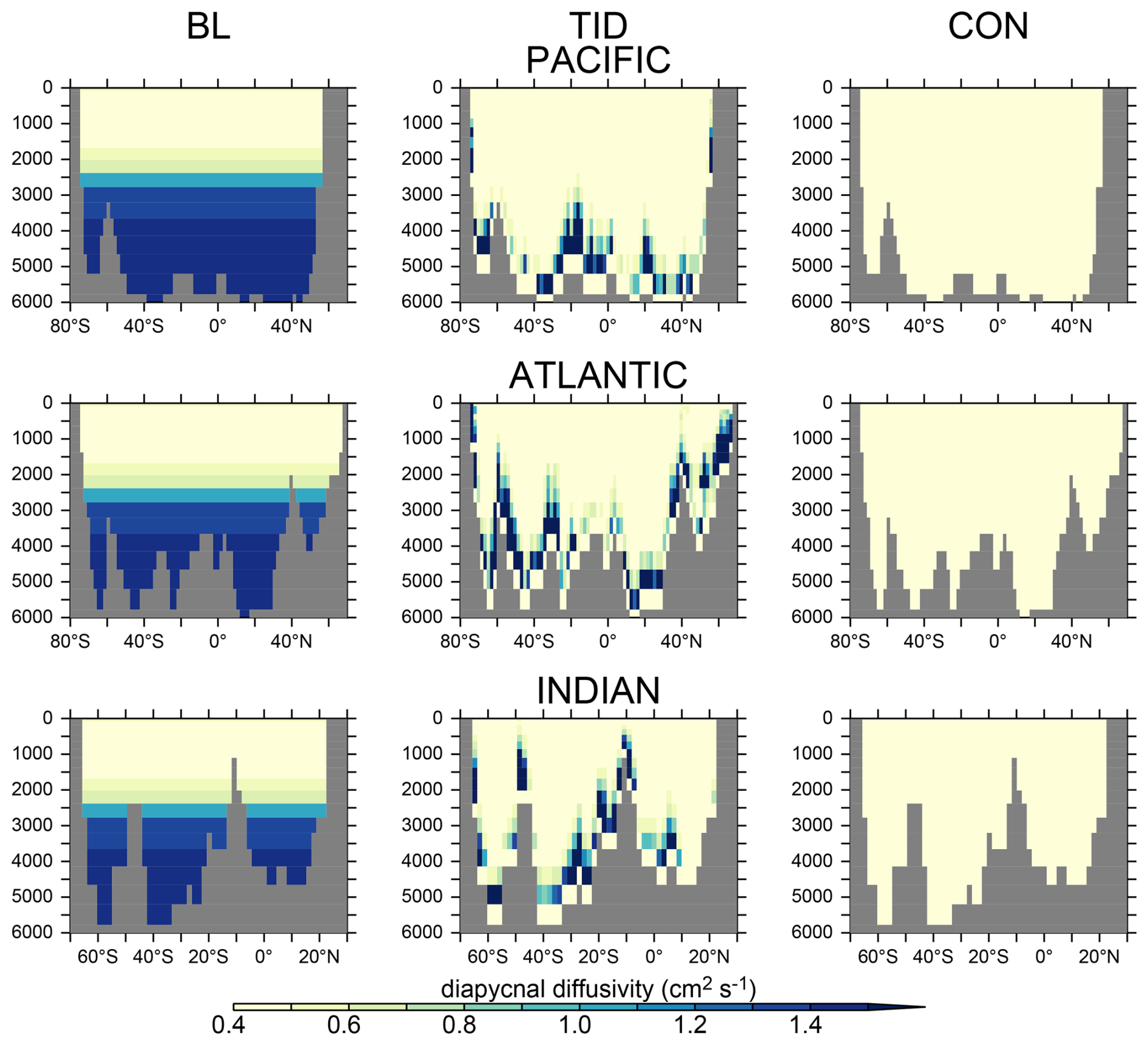
Figure 2 Longitudinal transects of diapycnal diffusivity at 150° W (Pacific Ocean), 30° W (Atlantic Ocean) and 65° E (Indian Ocean) for the three mixing parametrisations. See Table 1 for background k_v values.

Note that a linear advection scheme is required for TMM matrix extraction, thus the three vertical mixing models were produced with a linear third-order advection scheme (Quicker; Holland et al., 1998; Griffies et al., 2008) as described in Kvale et al. (2017). Kvale et al. (2017) demonstrated near equivalence in biogeochemical solutions using the transport matrices extracted with this approach, and those obtained with the non-linear Flux Corrected Transport advection scheme (Weaver and Eby, 1997) employed with the standard fully coupled UVic ESCM.

2.3 Biogeochemical parameter optimisation

Biogeochemical parameter optimisation was conducted on each of the BL, CON, and TID matrices following the framework of Kriest et al. (2017), implemented for UVOK (Yao et al., 2019). This optimisation is represented in Fig. 1 as work flow step D. The model parameters were calibrated using annual mean global misfit to World Ocean Atlas (WOA) phosphate, nitrate, and oxygen data (Garcia et al., 2010a, b). The parameters selected for optimisation are:

1. the initial rate of detrital particle sinking (w_D,0; Eq. 2)

2. the rate of increase of detrital particle sinking (wdd) with depth (Eq. 2)

3. the ordinary phytoplankton maximum growth rate parameter (a; Eq. 3)

4. the ordinary phytoplankton N uptake half-saturation coefficient (k_N, Eq. 5)

5. the phytoplankton light attenuation coefficient (k_c; Eq. 6)

6. and the molar nitrogen-to-oxygen molar ratio for organic matter degradation and production ($R_{-\mathrm{O}:\mathrm{N}}$).

Calibrated parameter values are provided in Table 2. Particle sinking parameters, the $R_{-\mathrm{O}:\mathrm{N}}$ ratio, and the N uptake half-saturation coefficient were chosen for optimisation because deep ocean nutrients and oxygen are known to be sensitive to them (Kriest et al., 2017, 2020). The light attenuation coefficient and the phytoplankton growth rate were chosen because the biogeochemical response to climate change is suspected to be sensitive to them as warming and stratification alter growth limitation regimes (Kvale and Meissner, 2017; Flynn and Skibinski, 2020).

Detrital sinking in the model is parametrised to increase with depth (z) as:

$$\begin{array}{}\text{(2)}& w_{\mathrm{D}}=w_{\mathrm{D},\mathrm{0}}+wdd\times z.\end{array}$$

Phytoplankton maximum growth rate (J_max) is parametrised as a modified Eppley curve (Eppley, 1972) and is a function of seawater temperature (T) in Celsius, an e-folding temperature parameter T_b, and iron availability (u_Fe) modifying the growth parameter (a).

$$\begin{array}{}\text{(3)}& J_{\max }=a{\exp }^{\frac{T}{T_b}}{u}_{\mathrm{Fe}}.\end{array}$$

The phytoplankton maximum growth rate is further modified as a function of macronutrients, including nitrate, following Liebig's law of the minimum. The phytoplankton growth rate J is thus:

$$\begin{array}{}\text{(4)}& J=min(J_I,J_{\max }\times u_{{\mathrm{NO}}_{\mathrm{3}}^{-}},J_{\max }\times u_{{\mathrm{PO}}_{\mathrm{4}}^{\mathrm{3}-}}).\end{array}$$

J_I is the phytoplankton light-limited growth rate. $u_{{\mathrm{NO}}_{\mathrm{3}}^{-}}$ represents biological nitrate availability determined by the concentration of nitrate and the half-saturation coefficient k_N:

$$\begin{array}{}\text{(5)}& u_{{\mathrm{NO}}_{\mathrm{3}}^{-}}={\displaystyle \frac{\left[{\mathrm{NO}}_{\mathrm{3}}^{-}\right]}{k_{\mathrm{N}}+\left[{\mathrm{NO}}_{\mathrm{3}}^{-}\right]}}.\end{array}$$

Light attenuation by algae biomass is included in the calculation of photosynthetically available irradiance at each depth level:

$$\begin{array}{}\text{(6)}& \begin{array}{rl}I& =I_{z=\mathrm{0}}\mathrm{PAR}{e}^{-k_{\mathrm{w}}\stackrel{\mathrm{̃}}{z}-k_{\mathrm{c}}{\int }_{\mathrm{0}}^{\stackrel{\mathrm{̃}}{z}}(\text{OP}+\text{DZ})\mathrm{d}z}\\ & \cdot (\mathrm{1}+a_{\mathrm{i}}(e^{-k_{\mathrm{i}}(h_{\mathrm{i}}+h_{\mathrm{s}})}-\mathrm{1}\left)\right)\end{array}\end{array}$$

where PAR stands for the photosynthetically available radiation, k_w, k_c, and k_i are the light attenuation coefficients for water, ordinary phytoplankton (OP) and diazotrophs (DZ), and ice, $\stackrel{\mathrm{̃}}{z}$ is the effective vertical coordinate, a_i is the fractional sea ice cover, and h_i and h_s are calculated sea ice and snow cover thickness. See Keller et al. (2012) for a complete set of model equations.

Parameter optimisation was performed using the CMA-ES search algorithm to minimise the global misfit against the aforementioned datasets (Kriest et al., 2017). Over the calibration, the CMA-ES algorithm “evolves” towards an optimal parameter combination for each of the 3 physical model configurations (see an example search path in Fig. 3). The CMA-ES search space can both widen and narrow from generation to generation. Parameter bounds are prescribed based on a combination of a literature survey and expert knowledge; see Table 2. The calibration was ceased when the total minimum misfit stopped decreasing with successive generations.

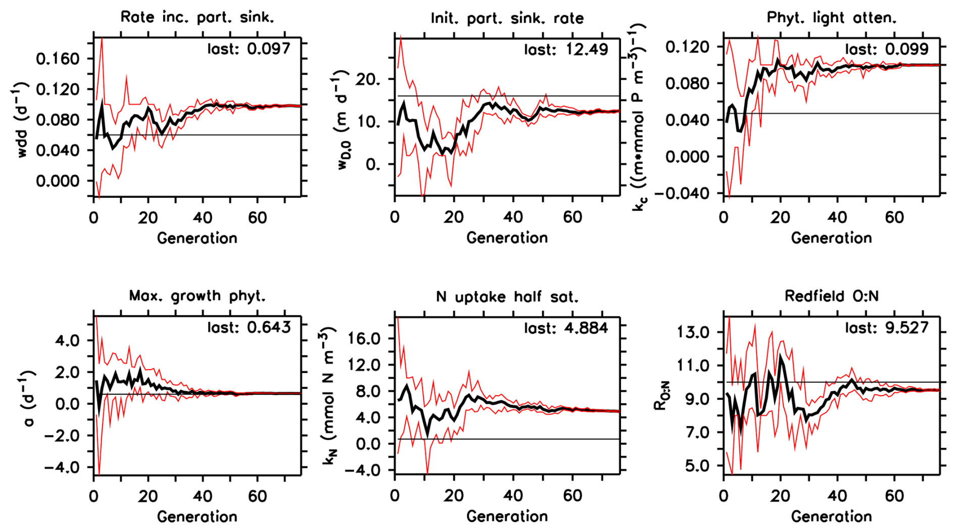
Figure 3 Resulting parameter values of the BL UVic ESCM biogeochemical parameter calibration, provided as an example of the evolution of the parameter optimisation. Thin black lines denote default model parameter values. Thick black lines are the average parameter values for all 10 individuals of a generation. Red lines are the maximum and minimum parameter values for each generation.

2.4 Transient simulations

The three optimal biogeochemical parameter sets determined by calibration within the offline TMM framework were then applied to the fully online coupled UVic ESCM, using the same physical configurations provided in BL, CON, and TID, and spun-up at least 10 000 years to physical and biogeochemical equilibrium at pre-industrial (year 1776) atmospheric boundary conditions. Atmospheric forcing encompasses CO₂, sulphate aerosol and chlorofluorocarbon concentrations, volcanic and solar radiative forcing, land ice and agricultural cover (Machida et al., 1995; Battle et al., 1996; Etheridge et al., 1996, 1998; Flückiger et al., 1999, 2004; Ferretti et al., 2005; Meure et al., 2006). This is work flow step E (Fig. 1). From year 1776, historical emissions forcing including fossil fuel and land use change CO₂ emissions is applied to year 2005, in work flow step F (Fig. 1). Solar insolation and wind forcing vary seasonally (Kalnay et al., 1996), but wind fields are fixed with respect to changing climate (Weaver et al., 2001). After year 2005, the model is forced with CO₂ emissions at a level consistent with the business-as-usual RCP8.5 atmospheric concentration scenario, to year 2100 (Riahi et al., 2007; Meinshausen et al., 2011). This scenario constitutes a rapid rise in emissions to year 2100, after which emissions stabilise and then linearly decrease to zero by 2250, and other forcings such as solar insolation and land use change remain at 2005 levels. This experimental set-up is designed to explore how the three equivalent models differ in their response to climate change.

3 Results

Our results are separated into five sub-sections, where the three vertical mixing models' equilibrated pre-industrial physical circulations are compared in Sect. 3.1. Calibrated biogeochemical model parameters are assessed in Sect. 3.2. The optimised pre-industrial ocean biogeochemistry of the three vertical mixing models is compared to observations in Sect. 3.3. Transient physical responses are described in Sect. 3.4. Model biogeochemical responses to transient forcing are described in Sect. 3.5.

3.1 Comparison of the BL, TID, and CON circulations

Here we present a suite of physical circulation metrics to compare model differences that arise due to application of the different vertical mixing schemes (Bryan-Lewis; BL, tidal mixing; TID, and a constant vertical diffusivity; CON). AMOC is maximum Atlantic Meridional overturning, calculated between the depths of 300 and 5000 m within the latitude range of 15 to 60° N and including the eddy-induced residual circulation. ACC is the maximum value of the zonal Antarctic Circumpolar Current at 68° W, integrated between 50 and 70° S and 0 to 6000 m depth. AABW is the zonally integrated minimum (anti-clockwise) meridional flow at 35° S, between 1000–6000 m depth and including the eddy-induced residual circulation. CDW is minimum (anti-clockwise) meridional flow of Circumpolar Deep Water in the Indo-Pacific basin, reported at 35° S and integrated between 1000 and 6000 m depth. Ideal age is the amount of time since a water parcel last had contact with the atmosphere (Thiele and Sarmiento, 1990; Koeve et al., 2015). These circulation metrics are selected for analysis due to their being previously demonstrated to exert control on ocean carbon storage, biogeochemistry, and primary production (e.g., Sarmiento et al., 2004; Ödalen et al., 2018; Sokolov and Rintoul, 2007) and because their responses to climate warming demonstrate strong variation across Earth System models (e.g., Ashton-Key et al., 2026; Meijers et al., 2012; Rintoul et al., 2026). Our definition of CDW effectively distinguishes the Indo-Pacific component of AABW in order to separately assess circulation-biogeochemistry correlations outside of the Atlantic. Globally averaged ideal age represents the integrated effect of the global overturning circulation on deep ocean water residence times.

Table 1 Pre-industrial circulation metrics from the three physical model configurations. Definitions are provided in Sect. 3.1 text.

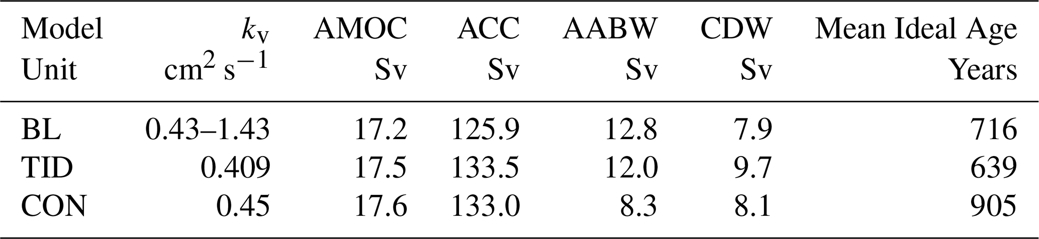
AMOC is very similar across all three model configurations (Fig. 4 and Table 1). It was hand-tuned by adjustment of the vertical diffusivity parameter value (or range of values in the case of the BL parametrisation) in each of the three vertical mixing configurations to obtain a maximum AMOC close to the middle of the range (17.5 Sv) of the observational estimate (15–20 Sv) of Cunningham et al. (2007). Depth profiles of AMOC are also similar across configurations, with the cell reaching 2.7 km depth in BL and TID, and 2.6 km deep in CON on basin average, with the maximum strength reached at about 800 m depth and 30° N in all models.

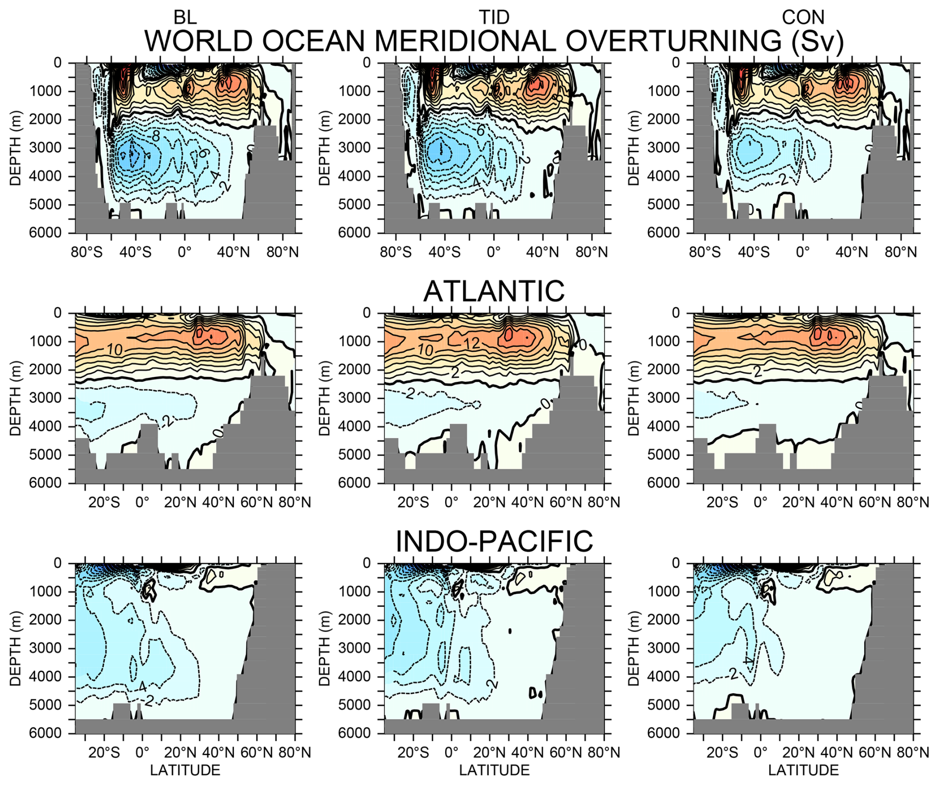
Figure 4 Average maximum pre-industrial meridional overturning in Sverdrups (globally averaged, top row) and by ocean basin for the three vertical mixing schemes. Clockwise rotation is in orange to red, anti-clockwise rotation is blue shading.

Similarities in the AMOC strength and depth do not extend to other circulation metrics, with larger differences apparent in the unconstrained Southern Hemisphere (Fig. 4). ACC strength is greater in TID and CON (133.5 and 133 Sv, respectively), and weakest in BL (125.9 Sv), Table 1). The globally prescribed wind fields are identical across models, but surface atmospheric temperatures are slightly different (13.08, 13.00, and 12.99 °C for BL, TID, and CON, respectively), resulting in small variations in wind-driven transport due the addition and parametrisation of wind stress anomalies using thermal anomalies (Weaver et al., 2001). AABW transport is strongest in BL (12.8 Sv) and weakest in CON (8.3 Sv), a factor 1.5 difference with respect to CON. More vigorous abyssal overturning circulation has been previously reported for higher values of diapycnal diffusivity (such as represented by the BL scheme) by Schmittner et al. (2005), who also reported globally stronger upwelling in the BL model than found when using the TID or CON configurations in the UVic ESCM. CDW transport strength is 23 % larger in TID compared to BL. Mean ideal ages vary by 42 % with respect to the smallest value, with CON being the oldest (905 years) and TID being the youngest (639 years).

Connectivity between upper and lower global overturning cells via CDW clearly impacts mean ideal age. The oldest deep water ideal ages (Fig. 5) in the CON simulation are consistent with this scheme having both weak CDW and the weakest AABW of the three parametrisations. The weak AABW, and strong and shallow AMOC in CON suggests a stronger isolation of deep water masses in this model configuration, with a rapidly-cycling upper ocean (including, a relatively strong ACC) and a relatively slowly circulating deep ocean. Likewise, the more “balanced” overturning in BL (estimated by AMOC-AABW yielding the smallest difference) suggests faster exchange of heat and carbon between the atmosphere and deep ocean, but the scheme does not have the youngest deep ocean on average because weaker CDW transport maintains a relatively older deep Pacific compared to TID. It is the TID scheme that has the youngest deep ocean, and mean ideal age, due to its vigorous CDW, which connects its upper and lower overturning cells of intermediate strength.

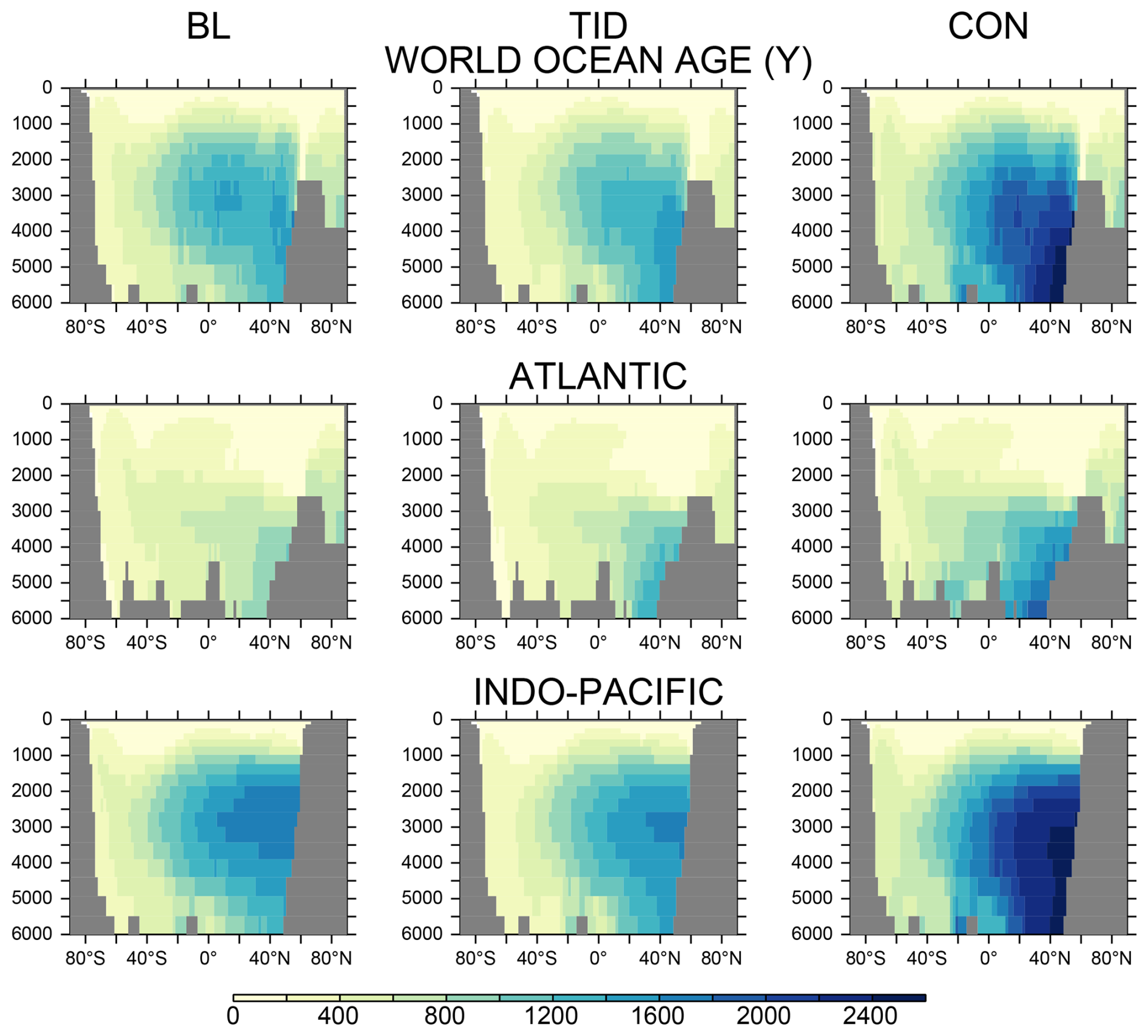
Figure 5 Average pre-industrial idealised water mass age in years (globally averaged, top row) and by ocean basin for the three vertical mixing schemes.

3.2 Comparison of the optimal parameter sets

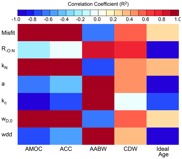
The optimal minimum misfit ranged from 0.57 (BL) to 0.62 (CON and TID). Nitrate fitness comprised the dominant fraction of the misfit, in an inverse relationship to phosphate (improvement to nitrate fitness resulted in reduction in phosphate fitness), a tradeoff that limited the total minimum misfit. Table 2 lists the optimal parameters from all three calibrations. Figure 6 examines whether the optimal misfit and optimal biogeochemical parameter values systematically vary with the models' physical circulation metrics using calculation of the square of the Pearson product moment correlation coefficient, R². The sign of the correlation indicates the slope of the relationship. It is important to note that our small sample size of only three points increases the uncertainty in our analysis, and we furthermore do not account for covariance, nor do we attempt to identify causal links. These correlations are provided as a means to explore systematic relationships between optimal biogeochemical parameter sets and minimum misfit with the models' physical circulation metrics, which could suggest some physical-biogeochemical parameter compensation. Optimal minimum misfit and biogeochemical parameter values are also plotted against physical circulation metrics, with linear regression slopes in Fig. A1. Minimum misfit demonstrates strong correlation with AMOC and ACC strength (R² values over 0.9, Fig. 6), where weaker overturning is associated with a lower misfit. This association suggests a compensation between physical model uncertainty and biogeochemical parameter uncertainty.

Of the optimal parameters, the phytoplankton growth parameter (a) shows the least variability (0.63–0.64 d⁻¹) between BL, TID, and CON. A value of 0.59 d⁻¹ is the original Eppley (1972) parameter value and this analysis demonstrates a similar value is robust for our model regardless of the vertical mixing parametrisation. The general high bias in our optimal parameter value could reflect a common bias in our model general circulation. Optimal values of a demonstrate a strong correlation with AABW strength, and strong anti-correlation with average ocean ideal age. Lower growth rates are associated with a shallower AMOC, a weaker AABW overturning, and older mean ocean ages.

Similarly, the $R_{-\mathrm{O}:\mathrm{N}}$ ratio also varies less than 4 % between BL, TID, and CON and is close to (but less than) the empirically-derived value of 10 (Anderson and Sarmiento, 1994). A robust $R_{-\mathrm{O}:\mathrm{N}}$ ratio is also broadly found in ocean observations (Körtzinger et al., 2001). The $R_{-\mathrm{O}:\mathrm{N}}$ ratio also demonstrates a strong anti-correlation with average ocean ideal age, where the smallest values correspond to the oldest ages. Smaller oxygen consumption ratios are required to compensate for slower circulation in order to fit simulated oxygen to contemporary observations, and at the same time more nitrate must be converted to its inorganic form when a sluggish model bias encourages denitrification in low-oxygen midwaters. These dual pressures may both be affecting the $R_{-\mathrm{O}:\mathrm{N}}$ ratio, as well as the air-sea equilibration of oxygen but not nitrate, and which may be sensitive to the general circulation. That the calibrated ratio for all three vertical mixing models is less than 10 is not altogether surprising as it was earlier found that multiple versions of the UVic ESCM have a sluggish deep circulation, particularly in the deep Pacific (Kriest et al., 2020).

Table 2 Resulting optimal parameter values for model calibrations. The prescribed parameter search range is the same for each calibration and is provided in parentheses in the BL line. Minimum misfit at end-of-calibration is given in the last column.

The remaining parameters display greater variability between vertical mixing parametrisations, and reflect the competing influences of upper ocean mixing and deep ocean circulation. The nitrate uptake half saturation coefficient (k_N) and initial detrital sinking rate (w_D,0) “export production” parameters vary by a factor of 2 and 1.6 compared to the lowest values, respectively, and demonstrate strong correlation with both AMOC and ACC strength (R² values above 0.9). Optimal w_D,0 values are at the upper bound of the prescribed range for TID and CON configurations, which might partly explain the relatively poorer misfit of these two mixing configurations (a larger prescribed upper range might have improved the misfit, and assumptions regarding the parameter value bounds may need to be re-evaluated in the future). The optimal k_N values in CON similarly approach the upper prescribed bound, but do not in TID. This might reflect the combined influence of AMOC (which is strong in both models) and upper-ocean diffusion gradients (stronger in TID). Light attenuation parameter k_c varies by a factor of 1.7 relative to the lowest value, and is strongly anti-correlated with AMOC strength, where a stronger AMOC is associated with weaker optimal light attenuation, and correlated with AABW strength, where a stronger AABW is associated with stronger optimal light attenuation. These relationships reflect the sensitivity of organic particle fluxes to light attenuation parameter value, where weaker light attenuation increases organic particle fluxes into the deeper ocean, below the clockwise cells of AMOC and the ACC, with their relatively fast nutrient recycling.

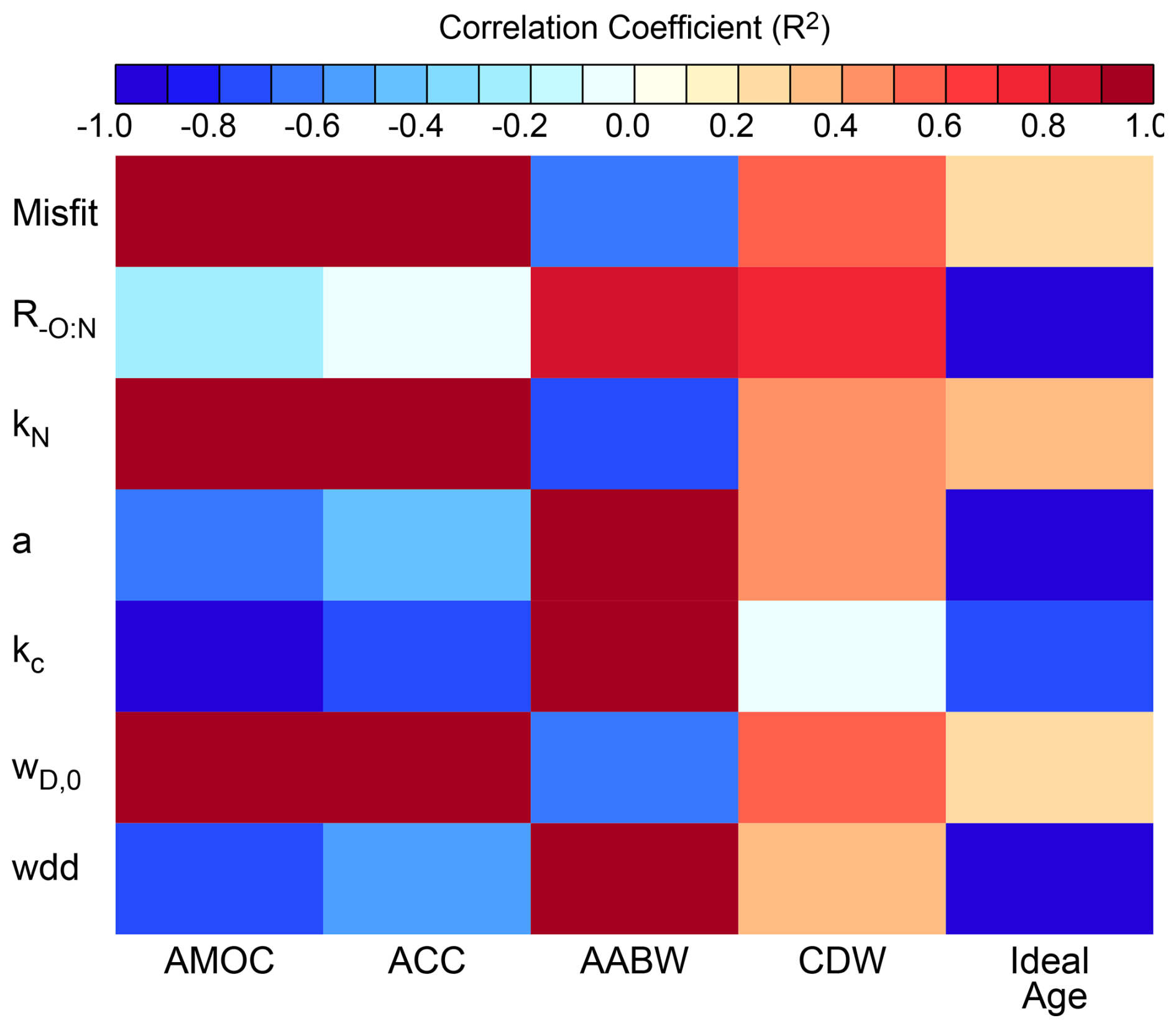
Figure 6 Mapping of optimal minimum misfit and optimal biogeochemical parameters to physical circulation metrics using calculation of the square of the Pearson product moment correlation coefficient, R² (colour coding).

The rate of increase of detrital sinking (wdd) varies by a factor of 1.6 relative to its lowest optimal value. It has the largest value in the BL calibration, which is surprising given this model is optimised with the lowest initial detrital sinking rates (w_D,0). Optimal values of wdd strongly correlate with AABW strength, where larger rates of increase for particle sinking are associated with stronger AABW overturning, and are strongly anti-correlated with ideal age. We speculate the relatively low initial detrital sinking rates control export production into the relatively vigorous and long-pathway AABW, but a rapid increasing detrital sinking rate regulates (and encourages) deeper nutrient remineralisation, which removes nutrients from the upper ocean more effectively (Kriest et al., 2020). This need in BL for upper ocean nutrient removal might relate to the relatively interactive upper and lower ocean water masses (recalling this configuration having very strong upwelling, as reported in Schmittner et al. (2005), relatively high vertical diffusivity, as well as the weakest AMOC, which suggests more “balanced” upper and lower circulation cells). In contrast, the CON calibrated rate of increase (wdd) is only roughly 60 % of that found using TID and BL, because this configuration produces a much older, slower-circulating, and more isolated deep ocean (and hence, a longer timescale of deep nutrient sequestration).

In summary, while the phytoplankton growth parameter and $R_{-\mathrm{O}:\mathrm{N}}$ ratio were robust across model calibrations, their optimal values were strongly anti-correlated with average ocean age and correlated with AABW strength. This is also the case for wdd, which showed a larger sensitivity to circulation differences. “Export production” parameters k_N and w_D,0, and total misfit are more sensitive to ACC and AMOC overturning strength, while wdd and k_c show strongest correlation with AABW strength. As was described in Kriest et al. (2020), faster overturning increases the resupply of nutrients to the upper ocean, which in turn requires stronger limitation on production parameters (which higher values of light attenuation and lower values of nitrate uptake half saturation achieve). Mean ideal age correlations with optimal parameters shows some (inverse) similarities with AABW strength, indicating the role of this transport pathway in regulating deep ocean age.

3.3 Residual uncertainties in calibrated pre-industrial biogeochemistry across the model ensemble

3.3.1 Basin mean nutrient and carbon depth profiles

All three model configurations retain similar biases in pre-industrial nutrient and carbon distributions in all ocean basins (Fig. 7) despite calibration, which result from shared biases in the general circulation (Kriest et al., 2020). Global overturning is generally too slow in the UVic ESCM (Schmittner et al., 2005; Kriest et al., 2020), and the resultant long deep nutrient sequestration timescales contributes a low bias in carbon and nutrients in the upper ocean, and a high bias in the deep ocean in all models, that cannot be overcome with calibration. This persistent circulation bias was also found by Kriest et al. (2020) using the biogeochemical model MOPS applied to the UVic ESCM circulation. However, our minimum model-observation misfits are slightly larger than what was achieved using MOPS (Kriest et al., 2020, their Fig. 4), which suggests the UVOK biogeochemical model is at least partly at fault for residual nutrient and oxygen misfits. Note that the application of the third order, linear advection scheme (Holland et al., 1998; Griffies et al., 2008) in these models has changed the general circulation compared to other previously published UVic ESCM simulations (Kvale et al., 2017), which apply a non-linear FCT advection scheme (Weaver and Eby, 1997). Further tuning of other physical parameters might be able to deepen the overturning circulation and reduce the model-data misfit across linear advection models. The objectives of this study are not, primarily, to produce a better model, but instead to highlight the window of transient responses arising from nearly identical (or only subtly different) pre-industrial models. No additional tuning of physical parameters was applied beyond adjustment of k_v for our study.

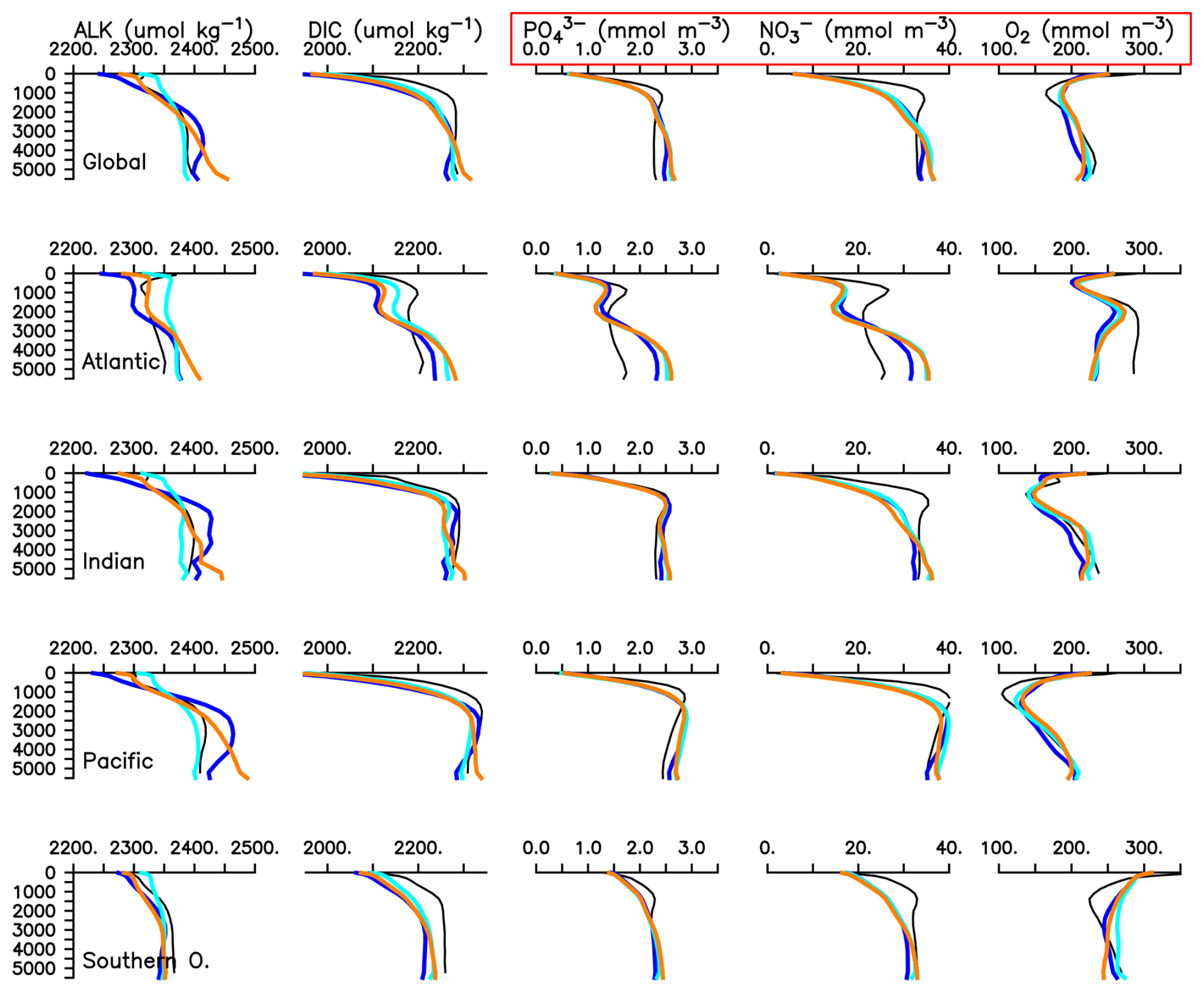
Figure 7 Biogeochemical tracer profiles for the optimal parameter sets (BL; dark blue, TID; light blue, CON; orange) of the online simulations. Black lines are observations (Key et al., 2004; Garcia et al., 2010a, b). The red box highlights the profiles targeted for calibration.

With respect to model ensemble variation in optimal, annually averaged nutrient distributions, surface concentrations in PO${}_{\mathrm{4}}^{\mathrm{3}-}$, NO${}_{\mathrm{3}}^{-}$ and O₂ are virtually identical between simulations both in global mean as well as by major ocean basin, a result of the models being calibrated against these variables. However, differences grow with depth, with up to 5 mmol NO${}_{\mathrm{3}}^{-}$ m⁻³ differences in the deep Atlantic, Indian, and Pacific basins (a result of different remineralization profiles arising due to both different mixing parametrisations and flux parameter values). Differences in the nutrient distributions optimised against are smaller than those resulting in the carbon tracers, which were not explicitly optimised for. Globally averaged surface alkalinity, an important determinant of buffer strength for air-sea carbon exchange, differs by just 3 % between models relative to the ensemble mean. The TID model performs best with respect to surface alkalinity, with a global average of 10 µmol kg⁻¹ higher than the GLODAP estimate. But differences grow with depth across the model ensemble, resulting in a difference of more than 50 µmol kg⁻¹ in the deep Atlantic, Indian, and Pacific basins between TID and BL models. These differences arise due to differences in particulate organic carbon (POC) export production, from which CaCO₃ export production (and subsequent dissolution) is calculated. Dissolved inorganic carbon (DIC) concentrations also differ between simulations in both the upper and lower water column for all basins (by nearly 50 µmol kg⁻¹ at 1000 m and below 5000 m depths in the Atlantic, but by less than 30 µmol kg⁻¹ elsewhere).

3.3.2 Biological rates and common biogeochemical metrics

Table 3 compares key global biogeochemical metrics across the model and parameter ensemble at steady-state. Globally integrated net primary production (NPP) varies by a factor 1.7 relative to the lowest value. TID and CON parameter ensembles under-estimate annual NPP relative to independent estimates, while the BL simulation falls within the range of 40–60 Pg C yr⁻¹ from Carr et al. (2006). The greatest spatial variation in NPP is in the low latitudes (Fig. 8), which is a region where all models over-estimate NPP compared to satellite-derived observations (NASA, 2018). Searching our circulation metrics for relationships, we find that calibrated models' global average NPP is strongly anti-correlated with AMOC strength (R² below −0.9) and ACC strength (Fig. 9), with weaker upper ocean circulations associated with higher NPP. We speculate that the enhanced upwelling in the BL scheme contributes to these strong anti-correlations via equatorial nutrient pumping, mainly in the Eastern Tropical Pacific upwelling zone, but note that it is not the circulation per se so much as the compensation of biogeochemical parameters to the circulation contributing this association. Pre-industrial circulation and biogeochemical metrics are plotted with linear regression slopes in Fig. A2.

Table 3 Pre-industrial biogeochemical metrics from the calibrated model configurations. Oxygen, phosphate, and nitrate inventories regridded to the UVic ESCM grid from Garcia et al. (2010a, b). Suboxic volume is defined by oxygen concentrations below 5 mmol O₂ m⁻³ and is also calculated from Garcia et al. (2010a). Primary production from Carr et al. (2006). Nitrogen fixation from Luo et al. (2014). POC flux at 130 m depth from Lutz et al. (2007), Dunne et al. (2007). These estimates employ a combination of remotely sensed chlorophyll observations, sediment traps data, and modelling to estimate POC flux in the upper ocean (100–200 m). Deep POC flux from Honjo et al. (2008).

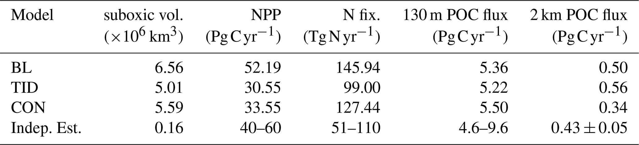
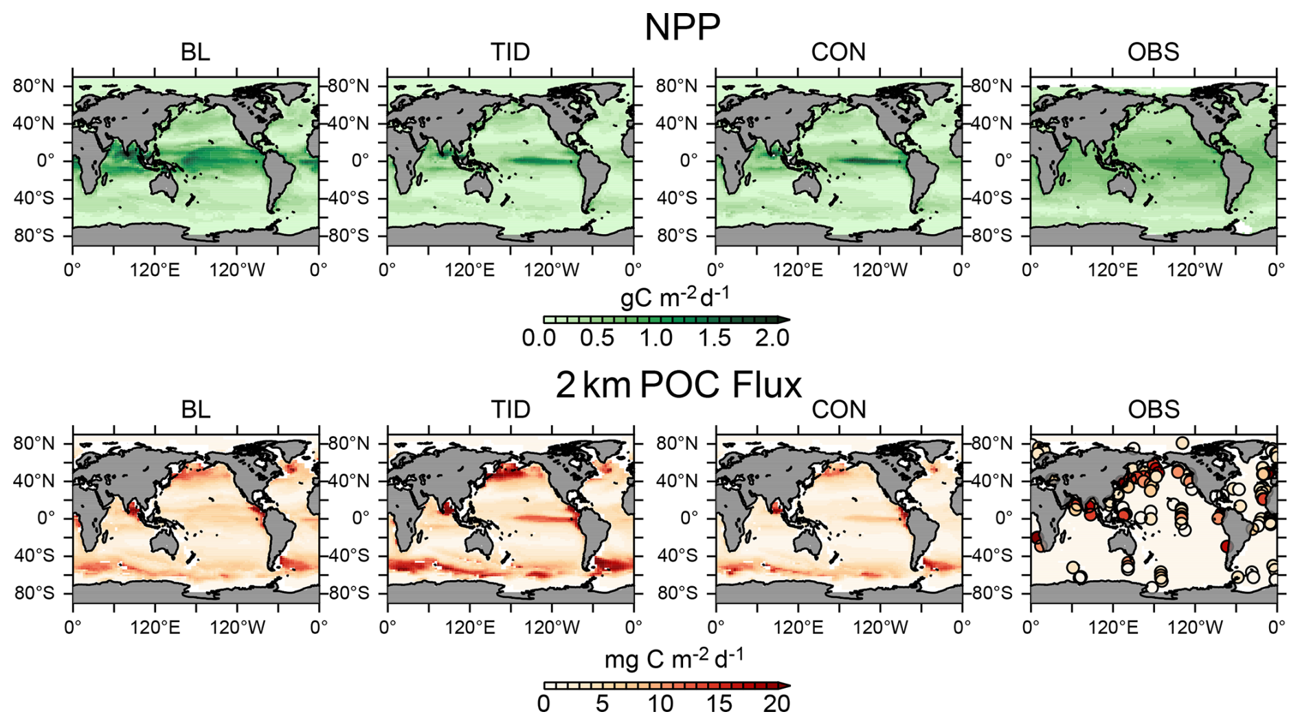
Figure 8 Top: Annual average pre-industrial depth-integrated net primary production (NPP) for all three calibrated models. Bottom: Annual average pre-industrial deep particulate organic carbon (POC) flux at 2 km depth for all three calibrated models. Observations are satellite-derived NPP climatology (2012–2018) (NASA, 2018), and 2 km depth sediment trap data (Honjo et al., 2008).

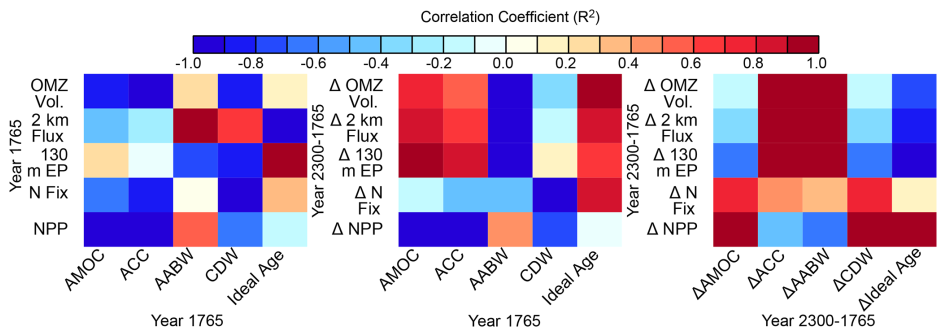
Figure 9 Mapping of pre-industrial circulation metrics (x axis, left and middle plot) and year 2300 change (Δ) in circulation metrics (x axis, right plot) against biogeochemical metrics (pre-industrial, y axis of left plot, year 2300 change in, y axis of middle and right plot) using calculation of the square of the Pearson product moment correlation coefficient, R² (colour coding).

Global mean particulate organic carbon (POC) fluxes vary by just over 5 % for POC at 130 m depth, but by a factor of 1.6 at 2 km depth, relative to the lowest value (Table 3). Like NPP, model variability in POC flux is large in the tropical ocean, but also in the Southern Ocean and along western boundary currents (Fig. 8). All models estimate upper ocean POC flux within a range of independent estimates (Table 3). The BL and TID models over-estimate deep POC fluxes with respect to the estimate of Honjo et al. (2008), while CON under-estimates the flux. All models show an over-estimate of deep POC fluxes in the Southern Ocean compared to Honjo et al. (2008) (Fig. 8). Greater model ensemble particle flux variation at depth reflects greater variability in deep-ocean circulation, as well as the calibrated flux attenuation parameter values, within the ensemble. The TID parametrisation (which represents the youngest deep ocean of the three models) yields the largest 2 km depth ocean POC fluxes, while the CON parametrisation (with the oldest deep ocean of the three models) yields the smallest deep ocean POC fluxes. Model calibration constrained the rate of particle sinking increase with depth to about 60 % slower in CON than in TID to compensate for the slower circulation. CON POC fluxes (and NPP) are higher than TID fluxes at the surface, but the organic particles have more time to remineralize above 2 km depth.

Searching our physical metrics for correlation, we find that the calibrated models' total global deep ocean POC flux is strongly correlated with AABW strength (Fig. 9), and strongly anti-correlated with mean ideal age. This is not surprising as these metrics describe the large-scale abyssal circulation, the biogeochemistry of which we have calibrated our model ensemble against. Intriguingly, the shallower 130 m depth POC fluxes show an inverse relationship to the deeper 2 km POC fluxes, with strong correlation with ideal age. This relationship does not appear clearly in CMIP6 models (Wilson et al., 2022, their Fig. 3), when comparing export production to POC fluxes at 1000 m depth across models of different physical and biogeochemical composition. But it does appear in calibrated models (Kriest et al., 2023, their Fig. 4), with the exception of calibration against only surface inorganic tracers.

Suboxic volume (here defined as the volume of water with oxygen concentrations below 5 mmol O₂ m⁻³) varies between 5.01 and 6.56×10⁶ km³ (a factor 1.3 variation with respect to the lowest model value, Table 3), whereas the average oxygen inventory varies by only a factor of 0.03 relative to the lowest model value (the latter a result of the calibration objective). The suboxic volume is overestimated by a factor of 35 across the model ensemble relative to the 0.16×10⁶ km³ estimate from the WOA data product of Garcia et al. (2010a). We find strong anti-correlation between suboxic volume and ACC strength, less (but R² still below −0.8) anti-correlation with AMOC strength and CDW, and only modest relationships with the other circulation metrics. Model bias in suboxic volume is probably an equal combination of biases in model physics and biogeochemistry (Kriest et al., 2020) and remains a major challenge for the discipline. Suboxic volume is also highly relevant to nitrogen cycling, because it is within these low oxygen regions that denitrification occurs.

Pre-industrial nitrogen fixation rates differ by about 47 Tg N yr⁻¹ (a factor of 1.5 relative to the lowest value) across the model ensemble (Table 3). Thus, strong differences in nitrate cycling result between models, despite similar total model pre-industrial nitrate inventories. Of the three models examined, TID performs best with respect to the independent nitrogen fixation estimate of Luo et al. (2014). BL and CON models over-estimate global nitrogen fixation. Nitrogen fixation remains poorly constrained by observations, with large remaining uncertainties (Landolfi et al., 2018). As with suboxic volume, we find a strong anti-correlation between calibrated models' total nitrogen fixation and CDW strength, and a lesser anti-correlation between ACC strength and nitrogen fixation, with stronger CDW and ACC flows associated with lower rates of nitrogen fixation (and reduced suboxic volumes). We speculate that these anti-correlations reflect the optimisation of parameters such as $R_{-\mathrm{O}:\mathrm{N}}$ and w_D,0 controlling the delivery of oxygen and preformed phosphate to the tropical oceans from the Southern Ocean, which determines the ecological niche of tropical nitrogen fixers (Kriest et al., 2020).

3.3.3 Summary and discussion of the pre-industrial uncertainty window

In summary, model calibration against global nitrate, phosphate, oxygen distributions cannot remove all biases from simulated pre-industrial biogeochemistry in our model ensemble. Residual misfits of 0.57 to 0.62 remain. This is due to a combination of biases found in our models' circulations, as well as the incomplete representation of real-world biogeochemical complexity by our relatively simple model parametrisations. In addition, those biogeochemical metrics such as NPP, deep particle fluxes, suboxic volumes, nitrogen fixation, and carbon and alkalinity distributions that were not included in the misfit objective show large variability across the calibrated model ensemble. We compared biogeochemical and circulation metrics across the optimal models and found strong anti-correlation between NPP, AMOC and ACC strength (i.e. upper ocean metrics), strong anti-correlation (deep) and correlation (shallow) between particle fluxes and ideal age and strong correlation (deep fluxes) and AABW (i.e. deep ocean metrics). Nitrogen fixation and suboxic volume are anti-correlated with metrics that connect the tropics to the Southern Ocean (i.e. ACC and CDW strength). These results suggest residual sensitivity of global biogeochemical features to relatively small variations in Southern Ocean circulation metrics after AMOC, oxygen and nutrient distributions are constrained to be as similar as possible across the model ensemble. Dissimilar pre-industrial biogeochemical rates resulting from biogeochemical parameter compensation for residual physical circulation differences across the model ensemble, despite similar nutrient profiles has implications for transient model responses to forcing and suggests large uncertainty with respect to how ecosystems and the ocean carbon sink might respond over both short and long timescales. We end by noting that our uncertainty estimates should be considered conservative in that we do not also account for measurement uncertainty in the biogeochemical fields that we use to calibrate our models.

3.4 Transient physical changes in the model ensemble

We next examine differences in model responses to the applied high-end CO₂ emission scenario. Atmospheric CO₂ concentrations increase uniformly until about year 2100 (Fig. 10). Despite identical emissions, the models diverge in their atmospheric CO₂ path after 2100, with a model ensemble spread of 62 ppm (ranging between 1425 and 1487 ppm) by the year 2300. The model with the greatest atmospheric CO₂ increase is BL, which is in part due to it having the smallest pre-industrial surface ocean buffer (calculated from the surface DIC : alkalinity ratio, not shown). We find that models with higher atmospheric CO₂ (and thus also temperature) have the smallest land carbon uptake over our simulations, reflecting a weakening of the land carbon sink with increasing global temperature (not shown).

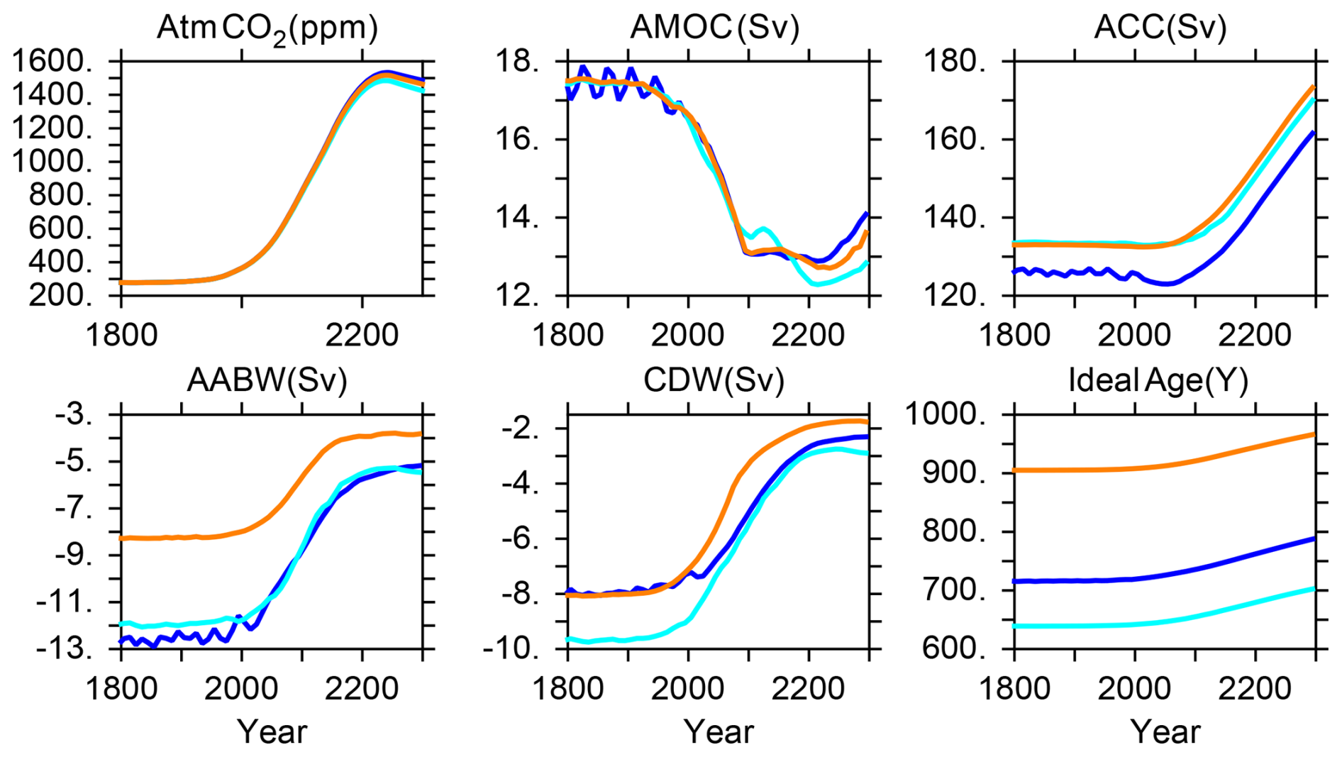
Figure 10 Global physical response to CO₂ emissions forcing for all three calibrated models. Dark blue is BL, light blue is TID, orange is CON.

With the exception of ACC circulation, global circulation metrics weaken, and ideal age increases, in all models (Fig. 10). Dependencies on vertical mixing parametrisation become most apparent after about year 2100; in general, the largest changes in ocean circulation metrics occur in models with the fastest pre-industrial circulation, suggesting the importance of vertical mixing-induced differences in the uptake and communication of anthropogenic heat into the interior and its effect on ocean density gradients. The BL overturning (with its high interior diapycnal diffusivities producing a relatively slow pre-industrial AMOC and relatively strong AABW) slows the least in AMOC by year 2300 and slows the most in AABW (also seen in basin-averaged plots of change in ideal age, Fig. 11). The CON model is less sensitive overall, with moderate responses in AMOC strength, ACC strengthening, AABW and CDW slow-down. The TID model (with its overall relatively strong pre-industrial circulation resulting in the youngest pre-industrial mean ideal age) shows the largest changes in circulation metrics for AMOC and CDW, and changes that are nearly equivalent to BL in AABW. In terms of absolute circulation strengths at the year 2300, we note convergence to smaller differences across the model range by year 2300 occurs in ACC, AABW, and CDW strengths, suggesting that the magnitude of the model responses are more sensitive to model forcing (which is identical across all simulations) than to choice of mixing parametrisation.

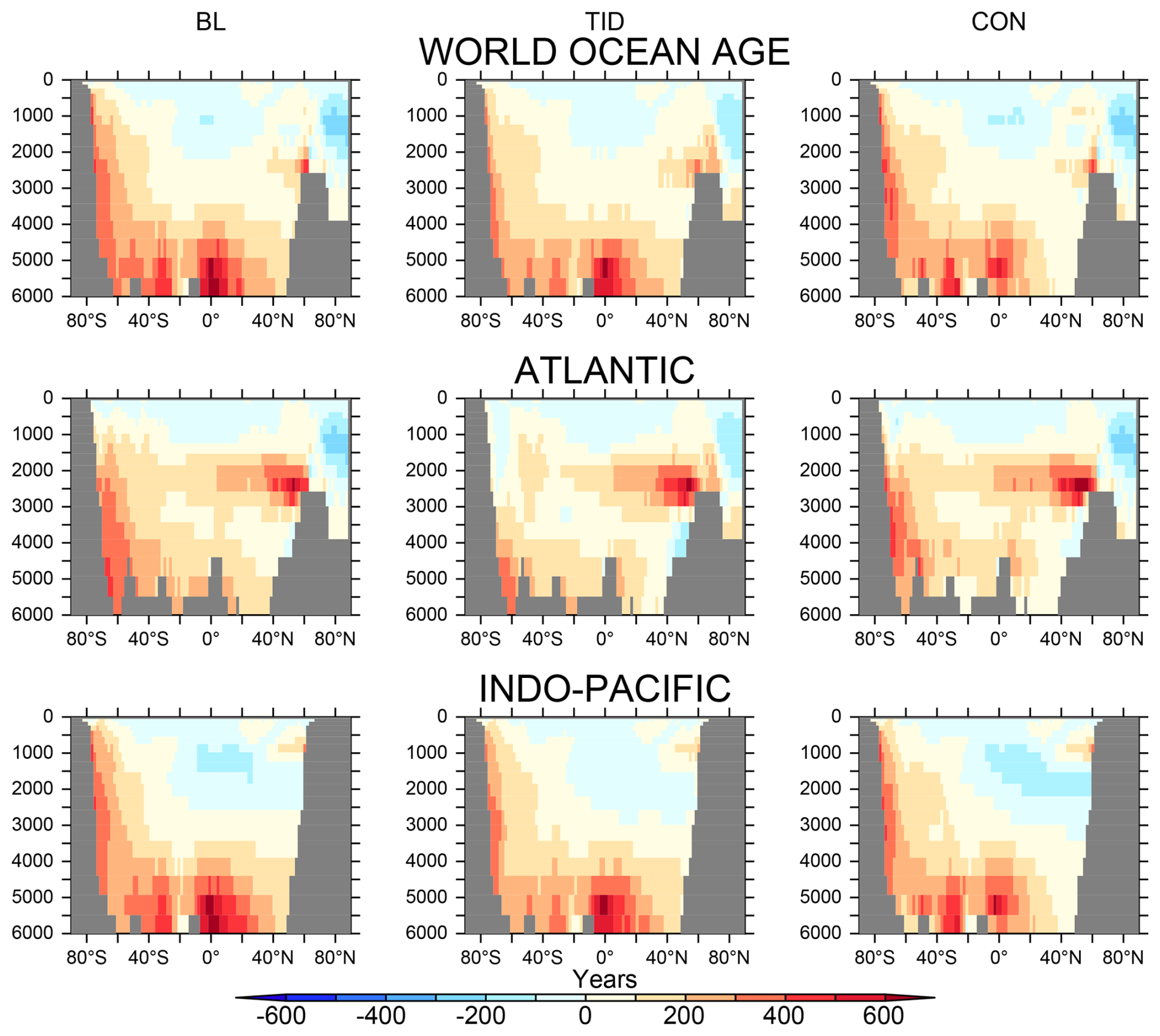
Figure 11 Change in ideal age (years 2300–1765) for the three vertical mixing schemes (BL, TID, CON).

3.5 Calibrated biogeochemical model responses to future transient forcing

We find a range of ocean biogeochemical responses to increasing CO₂ emissions and the associated global warming. The absolute range in NPP grows across models over the transient simulations (Fig. 12), and there results an 11 Pg C yr⁻¹ spread in the increase in global NPP by year 2300 across the model ensemble (Fig. 12). This is a smaller range in NPP response than found across the model ensemble for pre-industrial NPP. Similar to pre-industrial NPP, the strongest variation in change is in the low latitudes, where optimal model bias towards tropical NPP drives a stronger increase in NPP due to warming (Fig. 13; R²=0.995, Fig. 14). Increasing NPP with warming is a feature of the UVOK and other biogeochemical models, and is driven in part by an increase in upper-ocean nutrient recycling due to accelerating respiration, as well as warming of the high latitudes which both increases growth rates and reduces sea ice, increasing light availability (e.g. Schmittner et al., 2008; Taucher and Oschlies, 2011; Kvale et al., 2015, 2019; Landolfi et al., 2017; Laufkötter et al., 2015). A high bias in tropical production increasing sensitivity to warming also results in strong correlations in pre-industrial OMZ volume and rates of nitrogen fixation with change in NPP (Fig. 14). Pre-industrial biogeochemical and biogeochemical response metrics are plotted with linear regression slopes in Fig. A5.

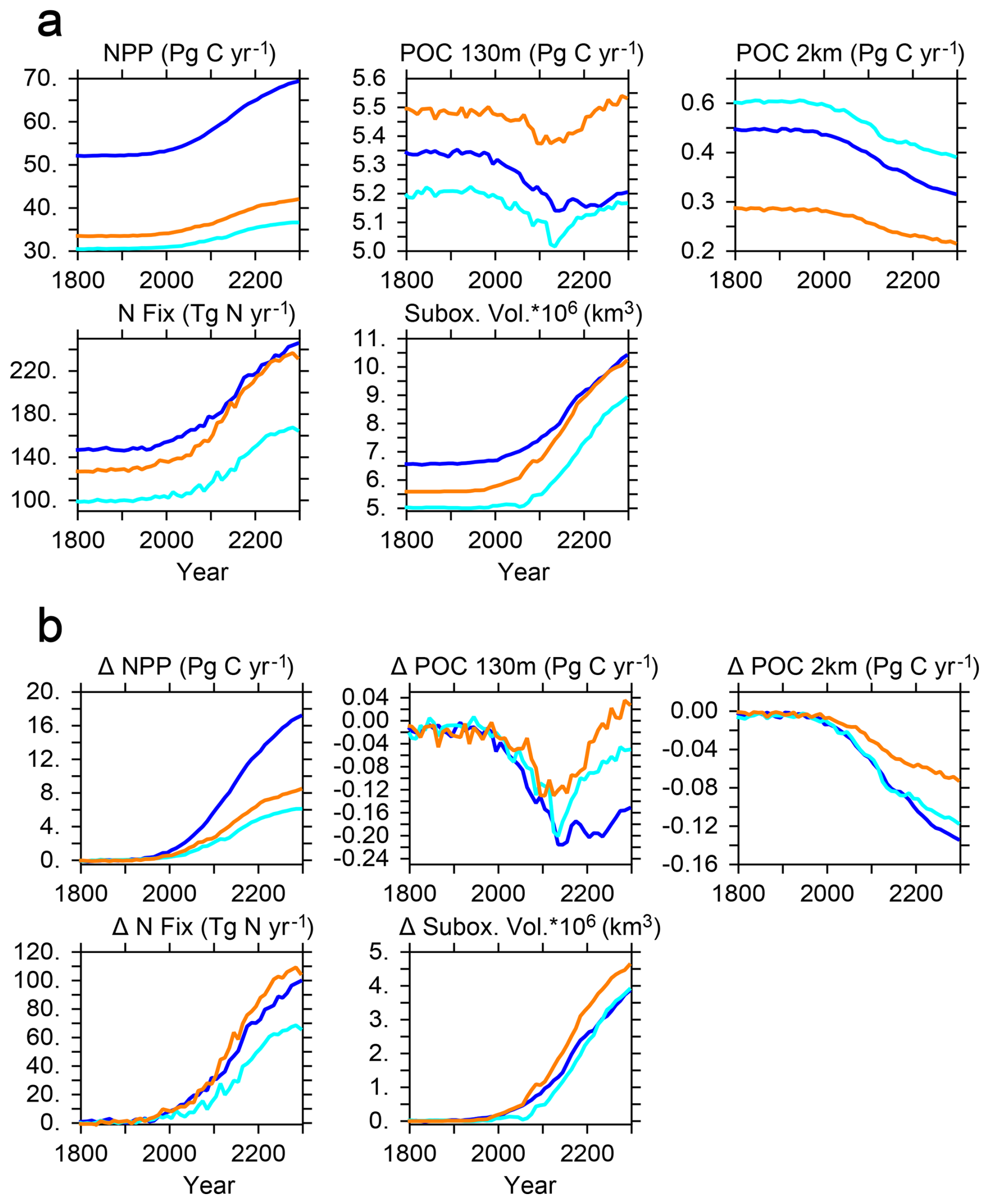
Figure 12 (a) Global biogeochemical metrics for all three calibrated models. Suboxic volume is calculated using a 5 mmol O₂ m⁻³ threshold. (b) Global biogeochemical response to CO₂ emissions forcing for all three calibrated models (Δ, year − pre-industrial value). Dark blue is BL, light blue is TID, orange is CON.

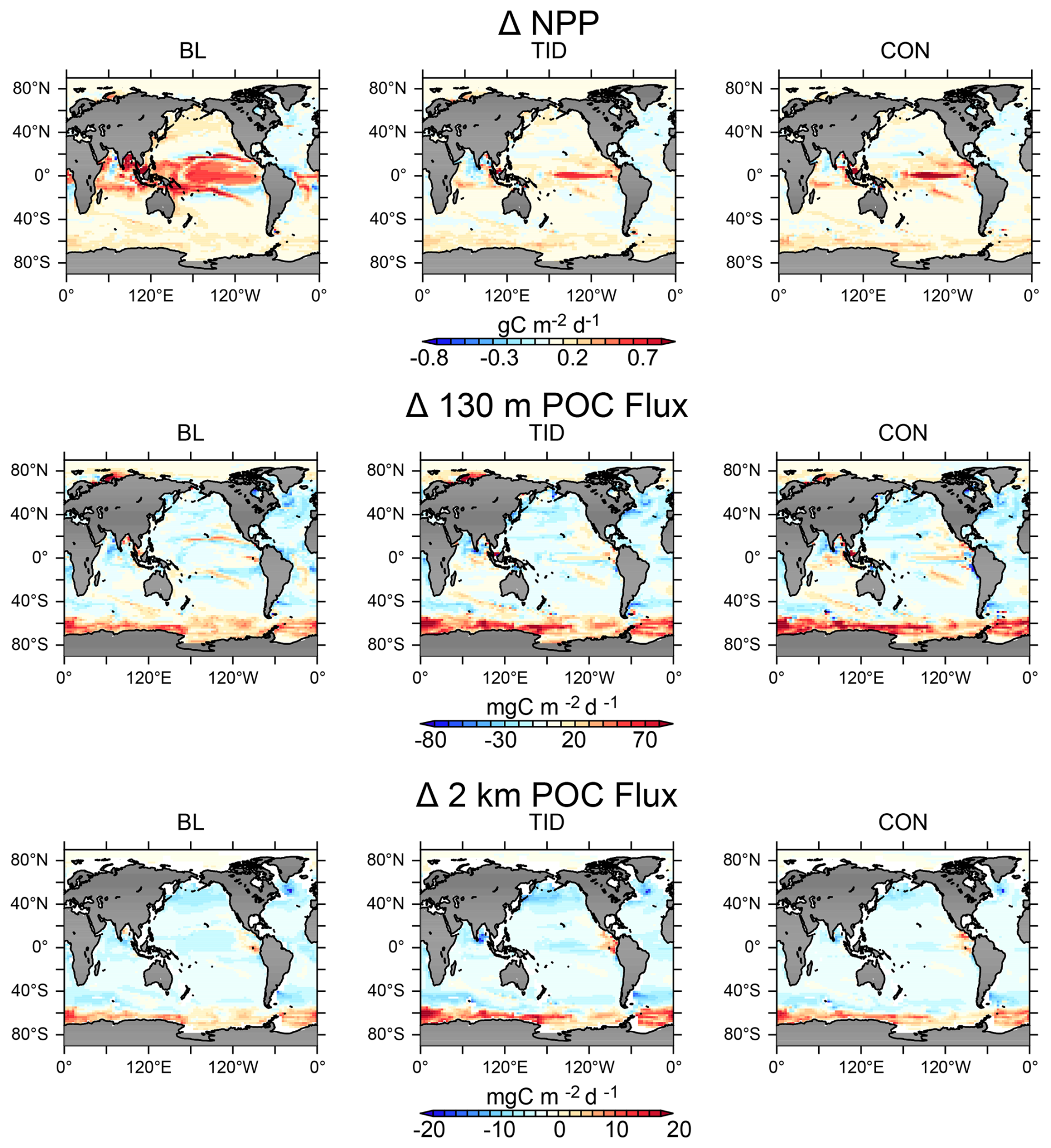
Figure 13 Top: Change in annually averaged depth-integrated net primary production (NPP, years 2300–1765) for the three calibrated models. Middle: Change (years 2300–1765) in annually averaged POC flux at 130 m depth. Bottom: Change in deep POC flux at 2 km depth.

With respect to the physical circulation, correlation patterns in global change in NPP are similar to those found for pre-industrial NPP, where the change in NPP is strongly anti-correlated with pre-industrial “upper-ocean metrics” AMOC and ACC strength (Fig. 9). Pre-industrial circulation and biogeochemical response metrics are plotted with linear regression slopes in Fig. A3. Pre-industrial AMOC and ACC strength can both therefore indicate a global NPP response with warming, where weaker pre-industrial AMOC and ACC is associated with a larger change in NPP. Change in NPP is strongly correlated with the change in AMOC strength, the change in CDW strength, and the change in ideal age, with the smallest weakening of AMOC and CDW resulting in the largest increases in NPP. We speculate that enhanced biogeochemical sensitivity to warming in models with circulations that are less sensitive to warming reflects the continuing influence of upwelling returning nutrients to the upper ocean, where they can be utilized under warming environmental conditions. More dramatic stagnation of global circulation limits nutrient resupply, thus limiting the response of ocean ecosystems to warming. However, our biogeochemical parameter calibration also contributes to this pattern because we have tuned our parameters to have weaker limitation of primary production in models that have weaker pre-industrial circulations. In particular, the initial detrital sinking rate (w_D,0) is slower in slower-circulation models, enhancing the availability of nutrients in the upper ocean. The weaker pre-industrial circulation contributes to lower sensitivity of the model physics to warming, but our tuning has enhanced the sensitivity of NPP to warming.

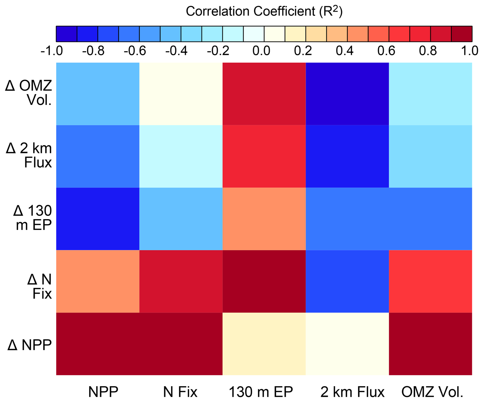
Figure 14 Mapping of pre-industrial biogeochemical metrics (x axis) and from pre-industrial to year 2300 change in biogeochemical metrics (y axis) using calculation of the square of the Pearson product moment correlation coefficient, R² (colour coding).

All models simulate a decline in both upper and deep ocean POC export fluxes before year 2100; Fig. 12) Trends are within the range found in CMIP and other models to year 2100 (e.g., roughly between −1 % to −20 %) (Bopp et al., 2013; Laufkötter et al., 2016). The model ensemble response spread grows after year 2100, but the range in absolute values show little change, and a small convergence in deep POC fluxes (Fig. 12). The BL mixing parametrisation produces a sustained long-term decline in deep and shallow POC fluxes, a result of the greater proportion of global NPP and export production occurring in the warm (and rapidly warming) low-latitudes, while the TID and CON parametrisations produce greater increases in POC fluxes in the cooler high latitudes (Fig. 13), although spatial patterns are broadly similar across all model configurations. Examination of the biogeochemical parameter ranges in Table 2 suggests variability in trend magnitude might arise from the spread in k_c, the light attenuation coefficient, which has previously been demonstrated to influence export production response to warming in the Southern Ocean (Kvale and Meissner, 2017). This model sensitivity arises because deeper primary production increases the amount of organic material exported to deeper levels. Indeed, Fig. 13 reveals the greatest increases in shallow and deep fluxes (calculated between years 2300 and 1765 at 130 m depth) occur in all models in the Southern Ocean, in contrast to the strongest increases in NPP which occur in the tropics. Increasing particle fluxes in the Southern Ocean is consistent with earlier findings using other models, e.g. Steinacher et al. (2010), Bopp et al. (2013), Laufkötter et al. (2016). In our models, there are only two plankton functional types and their relative competitiveness is not calibrated, so ecosystem complexity is not a driver of POC flux differences (e.g. Laufkötter et al., 2016).

Correlations found in pre-industrial shallow and deep POC fluxes with circulation metrics largely do not hold for simulated change in fluxes under global warming (Fig. 9). Circulation and biogeochemical response metrics are plotted with linear regression slopes in Fig. A4. The warming-induced changes in shallow and deep POC fluxes also do not demonstrate an inverse relationship with warming-induced circulation changes. There is closer agreement in the sign of the correlations of changes in deep and shallow fluxes with global warming against pre-industrial circulation metrics, where the change in shallow and deep fluxes with warming are correlated with pre-industrial AMOC and ACC strengths, and ideal age, and anti-correlated with AABW strength. Unlike NPP, pre-industrial bias in shallow and deep POC fluxes have lower correlation with shallow and deep POC flux responses to warming (Fig. 14). Instead, the response of shallow POC fluxes to warming is best (anti-)correlated with pre-industrial NPP, of the metrics we explore. With respect to both shallow and deep POC fluxes, the better predictors of flux responses to warming are the changes in circulation metrics with warming, where both shallow and deep POC fluxes are strongly correlated with the change in ACC and AABW strengths, and anti-correlated with the change in ideal age (Fig. 9). Thus it appears that with respect to POC fluxes, the largest changes occur in models with the largest changes in Southern Hemisphere-driven circulation metrics. We speculate that this is a product of model tuning, where models with Southern Hemisphere circulations that are more responsive to global warming were calibrated with faster rates of increase of particle sinking, therefore disproportionately exposing particle fluxes to deep ocean circulation slowdown (thereby reducing particle fluxes). These points highlight the difficulty in establishing simple, concrete relationships between physical and biogeochemical features that apply in both steady-state and transient environmental states.

The increase in global ocean volume where oxygen concentrations fall below 5 mmol m⁻³ exhibits a factor 1.2 model ensemble spread at year 2300, with respect to the smallest change (Fig. 12). However, the range in absolute suboxic volumes remains mostly unchanged (Fig. 12). Figure 15 displays change in O₂ concentrations at 300 m depth between years 1765 and 2300 for each model. Strong declines occur in the North Atlantic, North Pacific, and in the Indian and Atlantic sectors of the Southern Ocean in all models. The magnitude of the decline in the central North Pacific is particularly variable. As with POC fluxes, relationships demonstrated against circulation metrics for pre-industrial values do not hold for transient responses. In our optimal models, changes in suboxic volume with warming have a strong correlation against pre-industrial ideal age, and strong anti-correlation against AABW strength (Fig. 9). Like with POC, it is the response of the Southern-Hemisphere circulation metrics (ACC, AABW) that show the strongest correlations with change in suboxic volume with ocean warming. With respect to suboxic volume, the smallest changes occur in models with the largest declines in circulation metrics, i.e. the models that are the most physically sensitive to warming and had relatively strong pre-industrial deep circulations. This is likely due to compensating effects in the models, where the models showing the largest declines in deep circulation (which would increase suboxic volume) also show the largest declines in POC fluxes (which would act to decrease suboxic volume), to which the models with vigorous pre-industrial circulations use a $R_{-\mathrm{O}:\mathrm{N}}$ ratio calibrated to be particularly sensitive to changes in the POC flux in order to consume more oxygen in the pre-industrial deep ocean. This explains then why the pre-industrial suboxic volume is not useful in estimating the expansion of suboxic volume with warming, which is strongly anti-correlated with pre-industrial deep POC flux (Fig. 14). The potential for compensation between biogeochemical parameter tuning and physical circulation responses furthermore suggests that model biases that might lead to an over- or under-estimate of suboxic volume in the pre-industrial ocean might not equivalently over- or under-estimate future expansion of suboxic volume with warming.

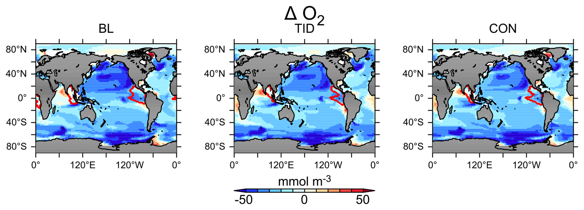
Figure 15 Change in oxygen concentration at 300 m depth (years 2300–1765) for all three calibrated models. Regions where concentrations are below 5 mmol O₂ m⁻³ at year 2300 are delineated in red to highlight regions in which denitrification occurs.

Changes in global nitrogen fixation rates similarly exhibit a 1.5 factor spread across the model ensemble response at year 2300, with respect to the smallest response (Fig. 12). Nitrogen fixation increases across our model ensemble, and by year 2100 is within the range of CMIP models (which do not agree on the sign of the trend, Wrightson and Tagliabue, 2020). The spread in absolute nitrogen fixation values grows within our model ensemble (Fig. 12). We find the models that over-estimated the observed global nitrogen fixation rate (BL and CON) also show the strongest increases in nitrogen fixation rate with warming, although the correlation between pre-industrial nitrogen fixation rate and change in this rate is modest (R²=0.74) in optimal models (Fig. 14). From our metrics, the strongest correlation that we found for the global increase in nitrogen fixation with warming is the pre-industrial POC flux at 130 m depth (Fig. 14), reflecting calibration of w_D,0 impacting remineralisation length scales, oxygen consumption and nutrient export. The pre-industrial shallow POC flux shows a modest (but weaker) correlation with the change in suboxic volume (the regions below 5 mmol m⁻³ support denitrification in our models), suggesting that trends in nitrogen fixation are regulated by more than trends in suboxic volume. Nitrogen fixation trends are strongly anti-correlated with pre-industrial CDW strength, which is similar to what we found for the pre-industrial values, suggesting that pre-industrial CDW is a useful predictor of nitrogen fixation response to warming.

Summary and discussion of the transient uncertainty window

In summary, we identify a range increasing with time of potential biogeochemical responses to climate warming and emissions in our model ensemble. Primary production, POC export, suboxic volume, and nitrogen fixation all demonstrate divergent trends with respect to pre-industrial global mean values. However, trends in all models largely share the same sign, which may be a result of using models with broad structural similarity (unlike CMIP, e.g. Bopp et al., 2013; Laufkötter et al., 2015, 2016; Wrightson and Tagliabue, 2020).

We find using simple regression correlations that response of a biogeochemical feature to warming may be predicted by a metric that showed no significant relation in the pre-industrial ocean, e.g. the response of shallow POC fluxes being strongly correlated to pre-industrial AMOC strength, but not to the change in AMOC strength, and with no strong correlation of pre-industrial shallow POC flux with pre-industrial AMOC strength. These shifting relationships between biogeochemistry and physics arise due to the constraints imposed by parameter calibration and inhibit identification of causality.

Pre-industrial NPP and NPP response to warming were found to have the most apparently robust correlations; to pre-industrial AMOC and ACC strengths, where a stronger pre-industrial circulation is associated with less pre-industrial NPP but a larger change in NPP with warming. However, this does not suggest that the AMOC and ACC are themselves drivers of the NPP response; more that calibration of the biogeochemical model compensates bias in the physical circulation that results in biogeochemical divergence with transient forcing. NPP has been documented previously as being driven by low latitude shallow respiration. Correlations in NPP have been previously analyzed; Kwiatkowski et al. (2017) concluded simulated tropical NPP sensitivity to ENSO-driven sea surface temperature anomalies is highly predictive of simulated tropical NPP responses at year 2100 to climate warming. Such an observation roughly encapsulates the combined influence of stratification on nutrient limitation, as well as the temperature-acceleration potential for upper ocean nutrient recycling in models. We suggest that their calculated emergent relationship works because of biogeochemical sensitivity encoded in each model; i.e., the NPP:respiration ratio, which is derived from biogeochemical model tuning against model physics.

4 Conclusions

Taken together, our model calibrations and forced transient simulations suggest that even with objective parameter optimisation against historical metrics, and starting from identical pre-industrial atmospheric CO₂ concentrations, and employing identical CO₂ emissions, uncertainty still remains with respect to future ocean biogeochemical responses to climate warming. This is because while models can be forced to perform similarly with respect to selected observations, such calibrations cannot constrain the sensitivity due to limitations of both data availability and the computational feasibility of including every process. Resulting calibrations therefore inevitably compensate for missing processes and metrics. In our simulations, we limited the calibration to global misfit against nutrient distributions and did not include biogeochemical rates in our metric. Rates are less observed and therefore more difficult to constrain at a global annual scale, which makes their inclusion in the model calibration framework problematic. We also left out carbonate production and dissolution terms and misfit against DIC and alkalinity distributions, which limited the calibration efficacy for carbon distributions and potentially related effects on atmospheric CO₂ in our transient simulations. Hence despite similar resulting misfits against global nutrient distributions across the model ensemble, unconstrained elements (such as upper-ocean buffer, net primary production, oxygen minimum zone volume, surface nitrate deficiency, and deep POC fluxes) remain. Differences in these unconstrained elements arise from resulting differences in calibrated model nutrient cycling (Yao et al., 2019), which can affect model transient response.

Likewise, it is possible (if not probable) that tuning to a different suite of physical metrics (i.e., not Northern Hemisphere overturning circulation but deep ocean ideal age, or Southern Hemisphere overturning) could produce a different optimal parameter ensemble, with a different range of model responses. Partitioning of carbon across biological and solubility pumps has been demonstrated to be sensitive to mixing parameters (Ödalen et al., 2018), therefore inclusion of other mixing terms in the model physical tuning might generate significantly different alternative solutions to our calibrations.

Our suite of emission-driven simulations demonstrate that differences in the poorly-constrained pre-industrial metrics can grow with time (and forcing), with an expanded uncertainty window for NPP by the year 2300. The other biogeochemical metrics that we examined, however, did not show substantial growth in their uncertainty windows to the year 2300. This is probably because the changes in circulation metrics largely converge across the model ensemble, and because the biogeochemical parameters have been calibrated to the circulation. By year 2300, the spread in the model response to climate warming and carbon emissions exceeds a factor 2.8 for net primary production, a factor 5 in shallow POC flux, a factor 1.7 in deep POC flux, a factor 1.5 in nitrogen fixation and 1.2 in suboxic volume, but the spread in absolute biogeochemical metrics across the ensemble has hardly changed relative to the pre-industrial equilibrium. Relative to the CMIP6 and CMIP5 model ensembles, our calibrated models have a smaller model response spread in NPP (Ryan-Keogh et al., 2025), POC fluxes (Wilson et al., 2022), and nitrogen fixation (Wrightson and Tagliabue, 2020), which is encouraging. Systematic calibration may partly close the open uncertainty window in ocean biogeochemical responses to climate warming.

Lastly, simple linear regression correlations are not necessarily robust on longer time scales. Application of our methods to a wider variety of models, to expand our sample beyond the three member model ensemble, would help to determine how robust our correlations are and whether they are useful for identifying mechanistic linkages. Our results suggest that drivers of model response under anthropogenic CO₂ emissions and climate change may be considerably different than the mechanisms governing steady-state physical-biogeochemical relationships or those possibly apparent at shorter timescales (considering, for example, the changing trend in shallow POC fluxes reported here). Thus, pre-industrial model biases may hold no predictive capacity in terms of determining model response bias.

Appendix A

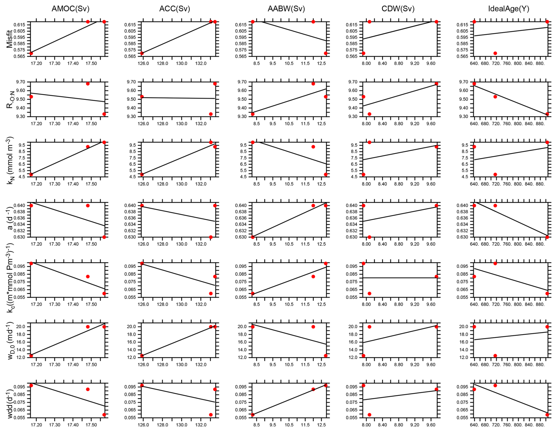
Figure A1 Calibrated model pre-industrial physical metrics (x axes) versus optimal biogeochemical parameter value or minimum calibration misfit (y axes); red dots. Linear regression lines; black line.

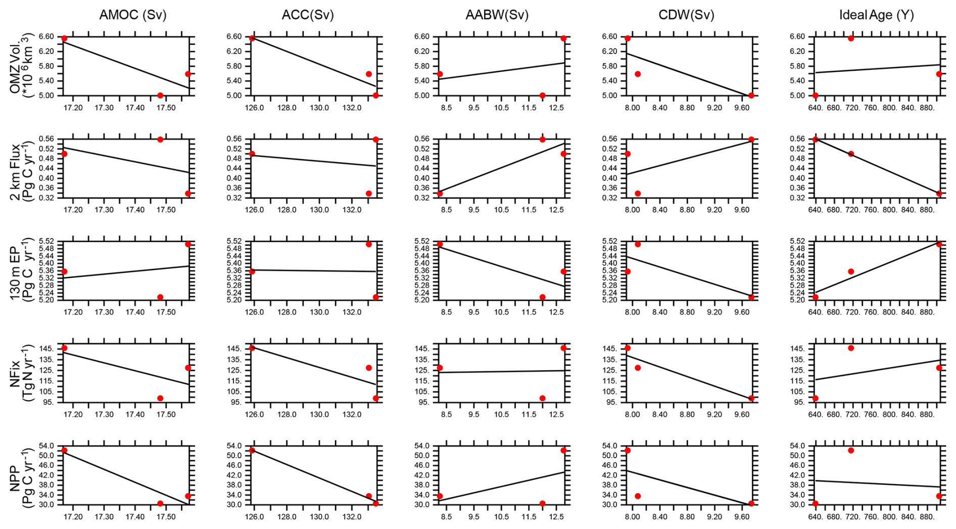
Figure A2 Calibrated model pre-industrial physical metrics (x axes) versus pre-industrial biogeochemical metrics (y axes); red dots. Linear regression lines; black line.

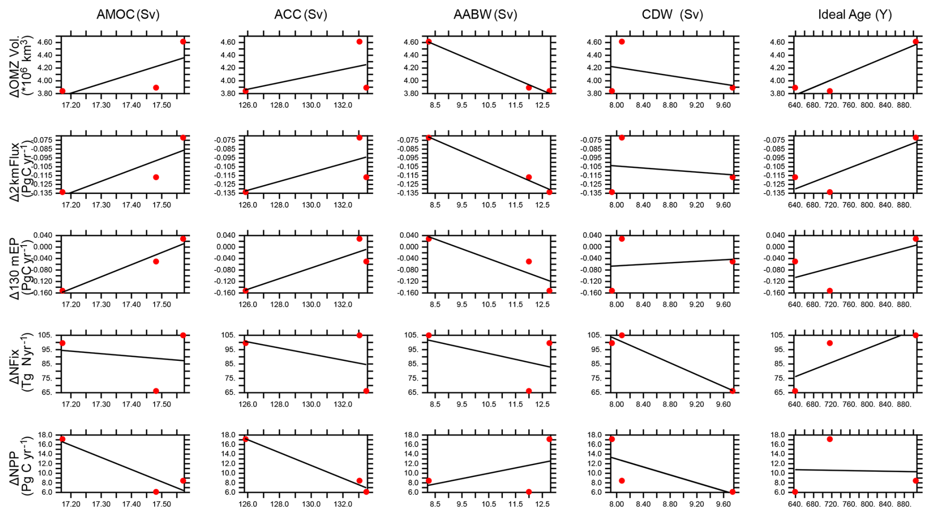
Figure A3 Calibrated model pre-industrial physical metrics (x axes) versus biogeochemical response (year 2300–1765) metrics (y axes); red dots. Linear regression lines; black line.

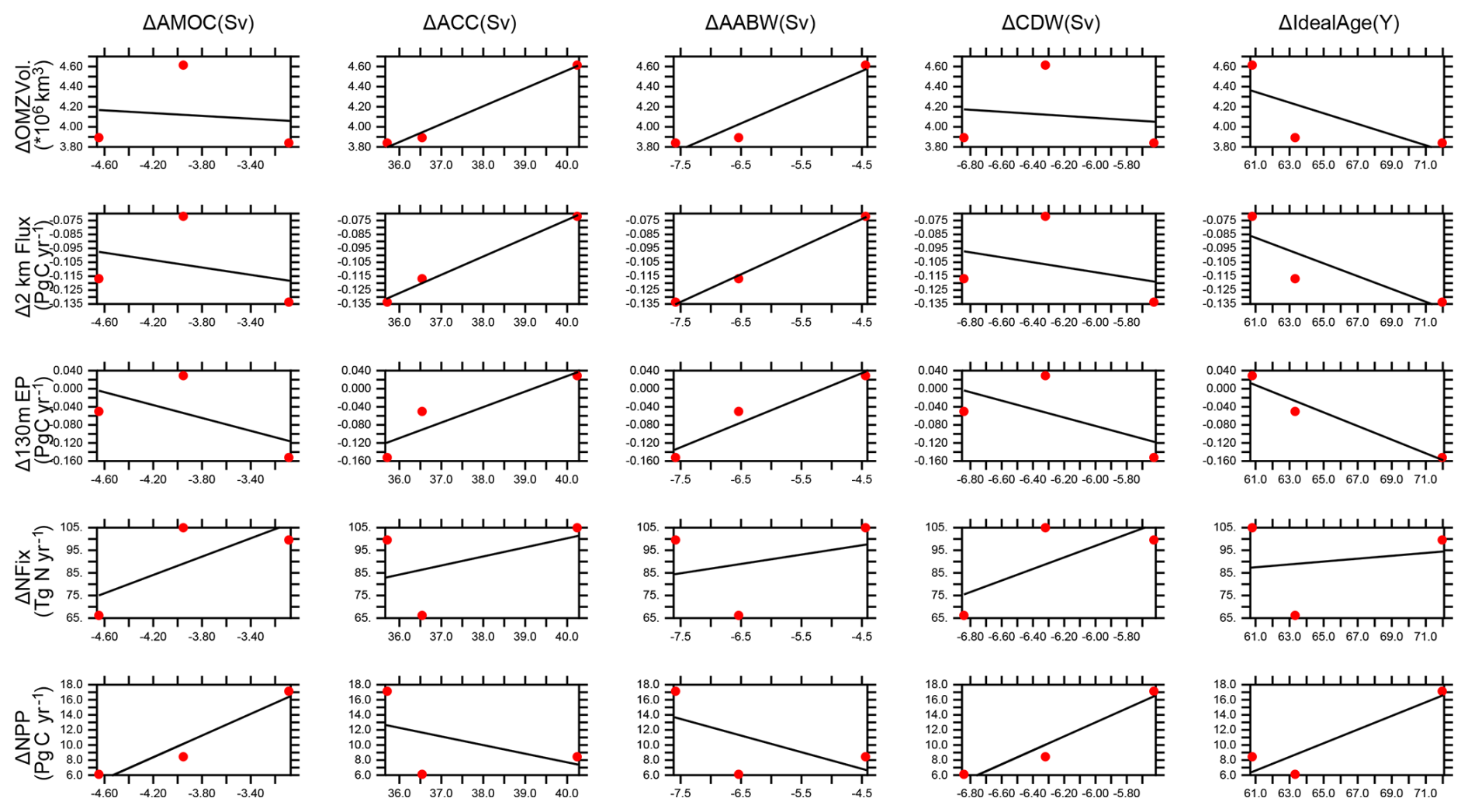
Figure A4 Calibrated model physical response (year 2300–1765) metrics (x axes) versus biogeochemical response (year 2300–1765) metrics (y axes); red dots. Linear regression lines; black line.

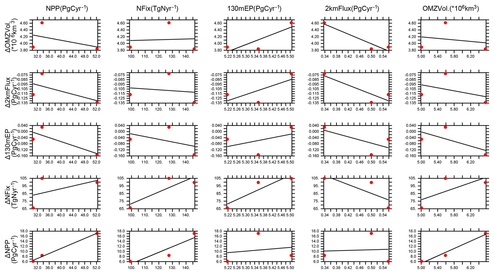
Figure A5 Calibrated model pre-industrial biogeochemical metrics (x axes) versus biogeochemical response (year 2300–1765) metrics (y axes); red dots. Linear regression lines; black line.